Underwater Sensor Network Simulation Tool (USNeT)
Kyriakos Ovaliadis
University of Portsmouth, Portsmouth, UK
Nick Savage
University of Portsmouth, Portsmouth, UK
ABSTRACT
A new Underwater Sensor Simulation Tool (USNeT) is proposed in this paper which has been designed and implementedassuming the conditions that affect underwater communication. This system provides real-time process based simulation and supports three-dimensional deployment. USNeT follows the object-oriented design style and all network entities are implemented as classes in C++ encapsulating threads mechanisms. Threads have been used because of the system need to handle multiple tasks. . Finally, the system has the functions to allow accurate visualization of the sensor nodes in a 3D manner and it presents a freely controllable camera that allows users to view the area from any angle.
General Terms
Underwater network simulation.
Keywords
Cluster, multithread, object-oriented simulation, energy efficiency.
1.
INTRODUCTION
This project proposes a simulator that focuses on UWSNs. The primary use of the simulator is to test the proof of concept for a specific energy efficient cluster routing algorithm. Since the simulator needs to simulate UWSN, the development of a model for an acoustic channel is required. The system also needs to be able to scale to a large number of sensor nodes and should be capable of modeling the energy state of each sensor in both transmission and reception state. Configuration options should include the number of nodes, the simulation time, the battery level, the data gather interval, the necessary variables for the communication process such as signal frequency, maximum transmission distance transmission rate, packet losses and errors and finally the variables for the cluster based scenarios such as the CH selection area, the suspension time of a node and the times a node has the ability to seek for a CH. The simulator should provide a graphical user interface (GUI) that allows the user to configure a simulation, run the simulation and then visualize the results. Moreover, the visualization scheme has to be understandable, usable and it must not decrease the performance of the simulator in term of scalability. In conclusion, the software should deliver the required functionality and performance to the user and it should not make wasteful use of system resources and should be able to evolve to meet changing needs [2],[3]. Table 1 shows a list of functional and non-functional requirements.
This paper is organized as follows. In Section 2, this paper briefly reviews some related work. In Section 3 the operation of a cluster based network is explained with the design methodology and the system architecture. In section 4 the
[image:1.595.317.544.256.486.2]implementations details of USNeT are presented. In Section 5, a simulation scenario based on the cluster algorithm has been chosen to present the operation of the USNet application. Finally, in Section 6, there is a discussion about the benefits of the application and some future research directions.
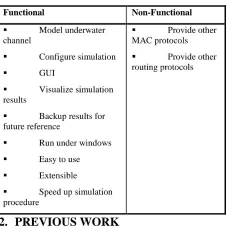
Table 1. Functional and non-functional requirements
Functional Non-Functional
Model underwater
channel
Configure simulation
GUI
Visualize simulation
results
Backup results for
future reference
Run under windows
Easy to use
Extensible
Speed up simulation
procedure
Provide other
MAC protocols
Provide other
routing protocols
2.
PREVIOUS WORK
Sensor network systems have been widely studied in the last decade and a lot of work has been completed on designing and developing sensors and communication systems. There are many network simulators that have been extensively used by researchers with different features. A short list includes NS2 [4], OPNET [6], OMNet++ [7] and TOSSIM [8] which are very popular in sensor network research community [9-12]. OPNET provides a comprehensive development environment supporting the modeling of communication networks and distributed systems. The simulation workflow has been adopted from our application due to the system’s simplicity (import configuration, run simulation, view results) and flexibility (duplicate the scenario, re-run simulation, compare the obtained results). NS2 is an open source application that provides the opportunity to view how the simulator has been designed, especially the part of the communication process between network components, the packet format and the event scheduler. OMNeT++ has been studied for future reference due to the modular architecture that it uses. The approach taken in this paper for designing applications is more understandable and easy to use. Finally, TOSSIM, a bit-level discrete event simulator and emulator of TinyOS [13], has also been studied for future reference mainly for its ability to simulate real sensor code.
in MATLAB [16-18]. However there are a limited number of reliable underwater simulation platforms which are proposed by the research community, compared with the terrestrial networks. In addition to this, most of them have been designed for specific experiments and it is difficult for other researchers to reuse the developed modules. The following simulators have been studied in order to investigate the underwater physical and MAC layer model implementation. Furthermore the MAC layer section of Aqua-Sim helped us to design and implement the ALOHA based protocol in our simulator.
P.Xie et al. developed a new UWSN simulation package called Aqua-Sim[1],[19]. This simulation tool follows the object-oriented design style of NS2, supports three dimensional modeling and it can simulate acoustic signal attenuation, propagation delays and packet collisions. Aqua-Sim integrates very easily the existing codesof NS2 and hasan adequate number of MAC and routing protocolsspecially designed for UWSN. Finally, because of the lack of a NS2 NAM animator to visualize 3D UWSNs, uses an additional tool, the Aqua-3D animator [20].
UWSim is also a simulator that has been used for underwater sensor network modeling. This simulator designed and implemented for testing scenarios specific to UWSN environments, such as low bandwidth, low frequency, high transmission power, and limited memory. The software development follows C# object-oriented programming and it is based on a novel routing protocol proposed by the developers. Currently, UWSim has support for a limited number of functionalities, it is custom-designed for a specific algorithm and it calls for further extensions to support a wide range of UWSN simulation scenarios [21],[22].
3.
NETWORK ARCHITECTURE
An underwater network is typically made up of many autonomous and individual sensor nodes that perform data collection operations as well as store and forwarding operations to route the data that has been collected to a central node. The main challenges of deploying such a network are the cost, the computational power, the memory, the communication range and most of all the limited battery resources of each individual sensor node [23].
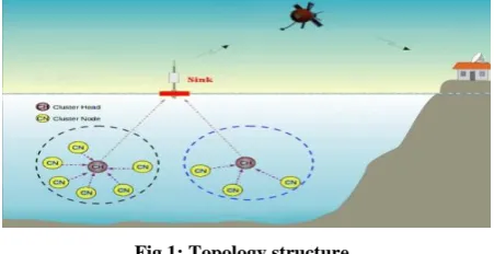
[image:2.595.55.281.619.735.2]Grouping sensor nodes into clusters has been used by researchers in order to extend the lifetime of an underwater sensor network. Many clustering algorithms have been proposed in the literature for UWSNs in the past few years [24]. These techniques vary depending on the sensor network deployment, the network architecture, the characteristics of the sensor and the master sensor node (Cluster Head) and the network operation model.
Fig 1: Topology structure.
A typical cluster based network consists of a sink (base station) and certain sensor nodes that are grouped into
clusters. In the structure, each cluster has a head, which are known as head-cluster or Cluster Head (CH). A CH may be elected by the sensors in a cluster or pre-assigned by the network designer. A CH may also be just one of the sensors or a node that is richer in resources. The CH is assumed to be reachable to all sensors in its cluster and it can broadcast messages to all sensors in this cluster. Sensor nodes perform two main functions: sensing and relaying. The sensing component is responsible for probing its environment to track an object or event. The collected data are then relayed to the sink through CHs in each level (tiers) [25]. The topology of such a system is shown in figure 1.
3.1
Design methodology
USNeT follows the object-oriented design style and all network entities are implemented as classes in C++ encapsulating threads mechanisms. Threads have been used because of the system need to handle multiple tasks in parallel and concurrently. This cannot be achieved with discrete event simulators such as NS2. In discrete event simulators, events that affect the state of the system are chronologically ordered into event queue, and event scheduler executes them one by one [26]. An event-driven simulator cannot execute multiple events at different nodes at the same time unless it uses a parallel discrete event or multithread approach [27].
In real life a wireless sensor node must do multiple operations without knowing the state of the other sensors at the same time. Each sensor operates independently doing tasks such as: sense a physical phenomenon, gather and store this information, send/accept information to/from other sensor node etc. In this simulator every entity (i.e. node, CH, sink etc.) of the system proceeds independently and simultaneously, providing a real-time process-based simulation. No sensor node waits for another node, they all proceed at their own rate completing their tasks.
The thread methodology gives the ability to design and implement the communication medium and protocol in an easier and more accurate manner, leading to the simulation working in a more realistic way. Using threads also improves the performance of the application and they do not incur significant overhead to implement [28].
3.2
Threads and multithreading issues
Multithreading is a technique that permitsa program to carry out multiple tasks concurrently by dividing it into multiple threads. Multitasking operating systems can do more than one thing simultaneously by running more than a single process. Similar to this, a process can do the same by running more than a single thread. Each thread is a sequence of instructions executed independently allowing a multithreaded process to perform numerous tasks concurrently. Multithreading via parallelism and scalability, offers you the possibility to take advantage of multiprocessors, including multicore and multithreaded processors. When a multiprocessor machine executes a multithreaded program the independed threads can run simultaneously (in parallel) on separate processors, exploiting the parallelism of the hardware[29]. On multicore processors and multithreaded processors, a multithreaded application's performance scales appropriately because the
cores and threads are viewed by the OS as
Fig 2: System architecture.
3.3
System architecture
The architect diagram of the application can be seen in figure 2. The diagram is composed by the basic routines and subroutines of the system. The visualization scheme of the application divides the graphical user interface from the simulation engine resulting in not reducing the scalability of the simulator. The major procedures will be explained in the section that follows.
3.4
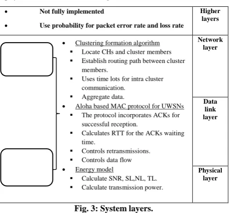
Joint –Layer design
A joint layer technique has been chosen to control the physical, data link and routing functionalities.
Not fully implemented
Use probability for packet error rate and loss rate
Higher layers
Network layer
Data link layer
Physical layer
Fig. 3: System layers.
The reason of following this approach is first of all because of the system energy consumption that must be optimized. Energy consumption is affected by all layers and strict layered design is not flexible enough to deal with this critical issue. On the other hand if the layers cooperate with each other this
can significantly reduce the overall system energy consumption [30].Secondly due to multithreading technique used and the need that most of the parameters should be accessible to multiple layers, it was more efficient to develop the protocol stack by joining the layers.
4.
IMPLEMENTATION
As already stated the application is divided in two major modules for scalability reasons: the user interface module and the computational module or simulation engine.
4.1
Interface
The main objective of the user interface is, first of all, to allow the user to import the necessary objects and variables of the model, then to provide the model’s simulation procedure animated on the screen, to start/stop simulation execution and to export the results.
4.2
Computational unit
This module consists of two major classes; the sensor class which defines the attributes of the sensor (node, sink, and CH) and the signal class which defines the acoustic link between sensors.
4.2.1
Sensor class
The sensor class simulates the full function of the sensor encapsulating all the necessary algorithms such as the communication algorithms along with all the other algorithms concerning the calculation of the energy consumption.
4.2.1.1
Distance calculation
ToA (Time of Arrival) technique is used to calculate the distance between sensors. ToA measures the distance between nodes using signal propagation time. Using the ToA technique, nodes transmit a signal to their neighbors at a predefined speed, which in the case of this environment is 1500 m/sec and wait for answers [31]. Their neighbors, in Clustering formation algorithm
Locate CHs and cluster members
Establish routing path between cluster members.
Uses time lots for intra cluster communication.
Aggregate data.
Aloha based MAC protocol for UWSNs
The protocol incorporates ACKs for successful reception.
Calculates RTT for the ACKs waiting time.
Controls retransmissions.
Controls data flow Energy model
Calculate SNR, SL,NL, TL.
Calculate transmission power.
Clustering Routine
[image:3.595.49.287.492.712.2]turn, send a signal back to them. Inter-node distance is computed by measuring the difference between sending and receiving times (round trip approach) [32].
The accurate calculation of the distance between sensors gives the system the ability to use the exact signal strength needed, saving with this way a significant amount of energy.
4.2.1.2
Energy consumption calculation
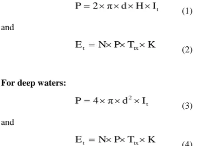
According to reference [33], the power level (P in Watts) and the energy consumed (Et in Joules), during transmission of a
K packets from a sensor node located at a distance d (d in meters) from the CH are given by the following expressions:
For shallow waters:
t
I H d π 2
P
(1)
and
K T P N
Et tx (2)
For deep waters:
t 2
I d π 4
P
(3)
and
K T P N
Et tx (4)
where N represents the number of hops towards the surface sink, Ttx (Ttx in second) represents the packet total
transmission time, K represents the total number of packets sent by the source node, It (It in Watt/m2) represents the
intensity at a distance point in the sea and H (H in meters) represents the distance (height) between the sea bottom and surface (only in shallow waters).
For commercial hydrophones, the energy needed to receive a packet is typically around one fifth of the transmitted energy [34],[35]. Thus the energy to receive a packet (Er in joule) is
t
r 15 E
E
(5)
4.2.1.3
Sensor and packet attributes
As already stated a sensor can be either a simple node member of a cluster or a cluster head. A sensor entity includes the following fields.
a. Sensor_id: a unique number given from the
simulator.
b. Cluster_id: when a cluster group is formed, this field takes the value of the CH sensor_id.
c. CH_id: when a sensor becomes a CH then this field takes the value of the cluster_id field otherwise remains null.
d. Battery level: initial battery level.
e. Energy field: calculates the remaining amount of energy.
f. Timer 1: used when the cluster is forming.
g. Timer 2: used in the communication process.
h. Distance: calculates the distance between sensor nodes.
i. Message counter: a sequence number – message id.
j. Packet counter: records the packet transmission efforts.
k. Buffer: flash memory for the data.
[image:4.595.53.249.229.374.2]A packet can be either a control packet used from the sensor as a connection request to a CH, an acknowledgment (ACK) or a packet with data. The packet includes two parts, the header and the payload (data). For simplicity reasons the packet’s header has been used to represent the control packets and ACKs, instead of having different types of packets.
Fig 4: Basic fields of a source packet.
The packet header which is 32 bytes long includes the following fields.
a) Sensor_id: a unique number (source id).
b) Cluster_id: when a cluster group is formed, this field takes the value of the CH sensor_id.
c) CH_id: when a sensor becomes a CH then this field takes the value of the sensor_id field otherwise remains null.
d) Target_id: destination sensor id.
e) Energy field: remaining amount of energy.
f) Timestamp: departure time of the packet.
g) Packet_id: a sequence number – message id.
h) Data size: the size of the payload.
4.2.2
Sorting signal class
The signal class is a very simple C++ sorting class which classifies the received packets (signals) and calculates the order that a sensor accepts these signals in relation of time. The simulator calculates the distances between sensor nodes, the propagation delay and the transmission time for a packet to reach a destination. The signal class, every time a sensor has to accept packets from different sources, uses the above-mentioned information, classifies the time each packet will propagate for and therefore gives to the destination sensor the ability to choose the order in which it will accept these packets.
4.3
Procedures and algorithms used
[image:4.595.382.487.607.734.2]There are two major algorithms that form the main routine of the system, the communication and the cluster algorithm.
Fig 5: Main procedure.
The communication algorithm is responsible for establishing the communication path between the wireless sensors, gathering the necessary data from the environment and the
Start
Clustering
Communicate
other sensors and sending this data to the upper level. The cluster algorithm is responsible for two very important tasks, the cluster formation and the selection of the CHs. Clustering is performed by assigning each sensor node to a specific CH node and all communication to (from) each sensor node is carried out through its corresponding CH node.
4.3.1
Main procedure
The clustering formation and communication process can be described in a few simple steps:
1. Firstly the nodes are deployed inside the space randomly.
2. When the deployment is finished each node sends a control packet seeking for a CH. The look up area is the sphere around the node with radii equal to the maximum transmission distance R.
3. First the sink and afterwards each CH according to the clustering algorithm sends back an ACK accepting these nodes to become members of the cluster.
4. When the clustering procedure is finished and each node belongs to a cluster team, the communication process of sending and receiving data begins. This time the node does not use the maximum transmission distance R but the exact distance.
5. Every node gathers data from the environment and after a specific time or when the buffer is full, sends this data to the CH of its team.
6. Every CH communicates only to each other and forwards the aggregated data to the sink which is the master CH.
4.3.2
Clustering procedure
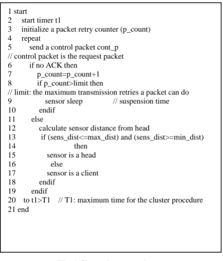
[image:5.595.316.545.70.337.2]This procedure is responsible for forming the cluster scheme by using the cluster algorithm. The basic idea of this algorithm is that each sensor, when the deployment is finished, sends a control packet seeking for a CH. If the sensor accepts an ACK then it connects to the specific CH otherwise it enters a different state such as the retry or the sleeping (suspension) state. A sensor can spend a significant amount of time seeking a CH. Therefore to avoid the total consumption of the sensor’s energy, after the retry state, where a sensor retransmits the control packet, it enters in a suspension mode. The suspension time is the period where a sensor sleeps without sending or receiving any signals and therefore without spending any energy. For further research, the suspension time can be altered by the user.This algorithm also has the responsibility of selecting the CHs for the next clusters at the lower tiers. This action is achieved when the algorithm chooses the CHs by taking into account the distance between the CH candidate and the already in place CH.
Fig 6:Clustering procedure.
4.3.3
Communication procedure
This procedure integrates two significant procedures which will be detailed over the next pages, the gather data and the transmit data procedures.
Fig 7: Communication procedure.
Generally a communication procedure has to deal with the receiving, gathering and sending of data. However it must take into account the two states that a sensor can be: the client state where a sensor is a simple node gathering data from the environment and the cluster head state where a sensor is a CH gathering data from both the environment and the other node sensors of the cluster team.
This procedure also cooperates very close with the cluster procedure in the case of a sensor node that loses the connection with a CH. When a sensor loses a connection then it must try to find another CH, meaning it needs to start the cluster procedure.
1 start
2 call gather data procedure 3 call transmit data procedure 4 if no ACK then
5 call cluster procedure 6 endif
7 end 1 start
2 start timer t1
3 initialize a packet retry counter (p_count) 4 repeat
5 send a control packet cont_p // control packet is the request packet 6 if no ACK then
7 p_count=p_count+1 8 if p_count>limit then
// limit: the maximum transmission retries a packet can do 9 sensor sleep // suspension time 10 endif
11 else
12 calculate sensor distance from head
13 if (sens_dist<=max_dist) and (sens_dist>=min_dist) 14 then
15 sensor is a head 16 else
17 sensor is a client 18 endif
19 endif
[image:5.595.316.545.403.523.2]4.3.4
Gather data procedure
[image:6.595.55.282.252.382.2]This procedure is responsible for gathering data from the environment, data from other sensors (if the sensor is also a CH), control packets and ACKs. The type of data received is checked at the waitForAck, waitForData and check buffer procedures. The amount of data gathered depends on the buffer size and the time period that a sensor collects data. If this time is exceeded then the sensor is forced to send the collected data, regardless of the buffer’s state. There is a possibility the buffer size will not reach the buffer limit when the sensor sends the data. This condition has been chosen because it is very important during research to get results in specific intervals depending, of course, on the research scenarios chosen by the researcher. However the period of gathering information can be changed by the user giving theability for further analysis.
Fig 8: Gather data procedure.
To avoid buffer overflow the procedure uses a buffer limit as a criteria of sending the information and not when the buffer is full. The buffer limit is chosen to be 500 bytes.
4.3.5
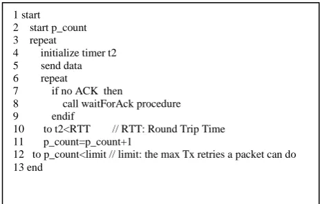
Transmission procedure
This procedure is responsible for transmitting the data to the upper or lower tiers depending on the type of data. For example if the node is a client sensor then the data can be a control packet as a request to a CH (upper tier) to join a cluster team, an ACK to a CH and finally information data.
Fig 9: Transmission procedure.
On the other hand if the node is a CH then the data can be either an ACK to the lower tier client sensor or an aggregating information data packet to the upper tier CH.This procedure is also responsible for the time period which a sensor is allowed to wait for an ACK until retransmission and how many retries a sensor can do. The number of retries it is not limited but it can be changed by the user for a further research purpose. The time period which a sensor is allowed to wait for an ACK
must be greater than the Round Trip Time (RTT). In our case, RTT is the length of time it takes for a packet to be sent plus the length of time it takes for an ACK of that packet to be received. The sensor calculates the RTT at the beginning of the cluster procedure, when it seeks for a CH to connect with.
4.3.6
WaitForAck and WaitForData procedures
As already stated the receiving data can be a control packet, an ACK, or information data. The basic idea of clustering is that each sensor can communicate and exchange information only with the CH of their cluster team. However there is a possibility for a sensor to receive a packet which is not wanted. The situation where a received packet is unwanted occurs when:
a. Duplicated packets have been received at the destination node.
b. Packets with a different target (destination) id have also been received at the destination sensor node.
[image:6.595.316.541.317.507.2]c. A simple sensor, that is required to collect data only from the environment, “listens” to data from other cluster team mates.
Fig 10: WaitForAck procedure.
These two procedures give a solution to these problems by checking the receiving data’s sensor-target and, with the help of the check buffer procedure, use the useful information, send the necessary ACKs and discard the unwanted data packets. Preventing a sensor from listening to packets with a different target id and thus saving more energy is a significant issue that needs further analysis. This subject will certainly be a part of our future research work.
Fig 11: WaitForData procedure. 1 start
2 call check buffer procedure 3 if control packet received then 4 if target_id=-1 then
5 sensor is a cluster head - send an ACK 6 else
7 discard data 8 endif 9 endif 10 end 1 start
2 call check buffer procedure 3 if control packet received then 4 if target_id==sensor_id then // target_id, sensor_id : sensor’s packet fields 5 ACK received
6 else
7 if target_id=-1 then
// when -1 is the value of the field, then the sensor is a head 8 sensor is a cluster head - Send an ACK 9 else
10 discard data 11 endif 12 endif 13 endif 14 end
1 start 2 start p_count 3 repeat
4 initialize timer t2 5 send data 6 repeat
7 if no ACK then
8 call waitForAck procedure 9 endif
10 to t2<RTT // RTT: Round Trip Time 11 p_count=p_count+1
12 to p_count<limit // limit: the max Tx retries a packet can do 13 end
1 start
2 initiate sample timer (tsm) 3 gather data from environment
4 if tsm<=Tsm then // Tsm: max time to gather data 5 repeat
6 call waitfordata procedure
7 to buffer>limit // the buffer has a limit of 500 bytes 8 call transmit data procedure
[image:6.595.53.285.502.650.2] [image:6.595.314.541.610.734.2]4.3.7
Check buffer procedure
Fig 12: Check buffer procedure.
The responsibility of this procedure is to check if the sensor’s buffer has data and the type of this data. This procedure cooperates very closely with the previous two procedures on the matter of discarding unwanted data packets and using or keeping the useful ones. Therefore one of the main tasks of this procedure is also the storage of this data which is the aggregated information from other sensors.
5.
Simulator application
5.1
Overview
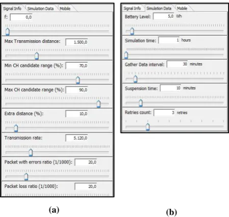
The graphical user interface (GUI) consists of two major components: a graphical display canvas, which could be expanded in case of viewing a large scale UWSN, and three property tabs for displaying node and signal properties. The researcher can easily use the input boxes or the roll bars to enter the necessary variables such as frequency, simulation time etc., according to a research scenario.
In the first property tab (see figure 13a) with the name “Signal info” the necessary variables for the communication process such as signal frequency, maximum transmission distance and transmission rate can be entered.
[image:7.595.370.491.98.298.2](a) (b)
Fig. 13: Signal info and simulation data tabs.
Furthermore, the maximum and minimum distance of the CH selection area, the packet error and the packet loss ratio can also be altered. In the second tab (see figure 13b) with the name “Simulation Data” the researcher can alter the simulation time, the sensor’s battery level, the data gather
[image:7.595.60.285.468.681.2]interval, the sleeping (suspension) time of a node and how many times a node has the ability to seek for a CH
Fig.14: Mobile tab.
Finally, the last property tab (see figure 14) with the name “Mobile” can be used when the scenario needs sensor mobility. In this tab a sensor’s coordinates can be altered while the simulation process is already in progress. The sensor’s coordinates are imported into the simulator via a spreadsheet which gives the ability to choose between random and definite deployment. It also gives the ability to store the deployment scenarios for future reference.The researcher can also speed up the simulation time by using the time acceleration roll bar. The user has the ability to gather the necessary results very quickly by accelerating the simulation time by a factor that starts from 1 up to 600 However the acceleration of the simulation time forces the system processes to perform more rapidly. When the system's load is heavy, meaning a large amount of calculations, the speed up procedure can cause a reduction in the computational accuracy. In order to overcome this problem the system must use either more computational power or decrease the amount of calculations in relation of time. Reduction of the number of calculations means fewer processes and fewer threads meaning fewer simulation entities.
5.2
Simulation scenario
A simple scenario has been chosen to present the operation of USNeT simulator. 50 nodes were randomly deployed in a field with dimensions 3000×3000×900 (m3), where 900 meters is the maximum depth of a sensor. The communication range for both the sensor nodes and the sink node was 1500 meters. The bandwidth of the data channel was set to 5 Kbps and the frequency range to 25 KHz. Each data packet with the packet header was 532 bytes long and the surface sink was set at the center of the sea surface. The simulation parameters are shown in the table 2.
Table 2. Simulation Parameters
Parameters Values
Number of Sensors 50 nodes
Frequency range 25 KHz
Max. TX distance 1500 m
Min CH candidate range 70%
1 start
2 check buffer procedure 3 if data packet received then 4 if data size!=0 then 5 if target_id=sensor_id then 6 store the data
7 send an ACK 8 endif
[image:7.595.315.543.673.762.2]Max CH candidate range 90%
Extra distance 10%
Packet with errors ratio (1/1000) 20
The deployment of this sensor network is shown in the figure 15.
Fig.15: 3D Canvas.
Fig.16: Simulation result tab.
The researcher has the ability to use the 3D capabilities of the USNeT simulator and therefore to have a more clear view of the cluster formation. There are a camera zoom and a view angle options and the projection of each cluster team is in a different color. The simulation results can be seen either on the “consumption” tab of the simulator (see figure 16) or on the exported file by using a spreadsheet application. The researcher can examine the outcome simulation data for each sensor separately, such as the energy consumption, the battery level, the successful transmitted/received packets, the successful transmitted/received ACKs and control packets. The detailed presentation of the results gives the researcher the ability of a more thorough analysis of the system.
6.
Conclusion
The main objective of our research is to design and test an energy constrained cluster based algorithm. For this reason a new simulator has been designed and implemented. It has a user friendly frontend environment, provides real-time process based simulation and it supports three-dimensional deployment. This simulator follows the object-oriented design style and all network entities are implemented as classes in C++ encapsulating threads mechanisms. Threads have been
used first of all because of the system need to handle multiple tasks. Since multi-core systems are now widely available and installed, doing multithreading parallelism is a simple but potentially efficient optimization for simulators performance [36]. Moreover, the benefits of our multithreaded application are responsiveness to the user and resource sharing which lead to a scalable and reliable simulation environment. When the application performs a long time tasks such as simulating large scale sensor networks, the amount of intensive calculations and I/O operations may slow down and possibly freeze up the system. This can lead to unreliable and, in the second case, no output results. However multithreading techniques allows the application to continue running even if part of it is blocked or is performing a lengthy operation. The number of sensors can also influence the simulation time and the memory usage. More memory usage means more frequent operations on the system resource, which is very time consuming. The creation of a thread does not require extensive system memory and the sharing of files and other resources, is simplified. Multi-threading enables you to make the best use out of the existing hardware resources and also enables simple resource sharing. Multithreading is also used to speed up the simulation time in relation to the real time. The simulator has the ability to run the simulation process faster than real time which makes it possible to observe the behavior of a network for large time durations. The designer does not have to wait for a long period during the evaluation phase of the system in order to monitor the sensor network performance. Finally, the researcher has the ability to test several scenarios very easily and quickly and compare and analyze the output results by using a simple spreadsheet application. The further work that must be done on this simulation tool is to broaden its ability to validate not only cluster-based but any other routing protocols such as flooding, multipath and miscellaneous [37]. At this stage this is difficult to be accomplished without making some edits into the source code. For example in order to use multipath routing the cluster algorithm must be subtracted and a new algorithm must be designed and major alterations to the rest of procedures must be done. However for a user who is familiar with the object oriented C++ programming language these alterations can be done very easily and quickly because the program code is understandable and easy to modify. Furthermore, the rest of the application which has to do with the user interface unit can be remained as it is with minor changes.
References
[1] P. Xie, Z. Zhou, Z. Peng, H. Yan, T. Hu, J.-H. Cui, Z. Shi, Y. Fei, and S. Zhou, "Aqua-Sim: An NS2 Based Simulator for Underwater Sensor Networks," in Proc. of MITS/IEEE OCEANS Conference, Biloxi, Mississippi, USA, 2009, pp. 1-7.
[2] H. Sundani, H. Li, V. Devabhaktuni, M. Alam and P. Bhattacharya,”Wireless Sensor Network Simulators A Survey and Comparisons,” International Journal Of Computer Networks,vol.,2., pp.249-265,Apr.2010. [3] E. Egea-Lopez, J. Vales-Alonso, A. S. Martınez-Sala, P.
Pavon-Marino and J. Garcıa-Haro, “Simulation tools for wireless sensor networks,” in Proc. SPECTS 2005, Philadelphia, PA, 2005, pp. 559–566.
[4] Network simulator, NS2. [online]. Available: http://nsnam.isi.edu/nsnam
[5] J. Chung and M. Claypool. NS by Example. Worcester
Polytechnic Institute. [online]. Available:
[6] OPNET, modeling and simulation. [online]. Available:http://www.opnet.com/solutions/network_rd/. [7] OMNET++, network simulation framework. [online].
Available: http://www.omnetpp.org.
[8] Simulating TinyOS Networks. [online]. Available: http://www.cs.berkeley.edu/~pal/research/tossim.html. [9] P. Wang, C. Li, and J. Zheng, “Distributed
minimum-cost clustering protocol for underwater sensor networks (uwsns),” in Proc. of the IEEE Int. Conf. on Communications (ICC07), Glasgow, Scotland, 2007, pp. 3510–3515.
[10]J. Llor, and M.P. Malumbres, “Underwater Wireless Sensor Networks: How Do Acoustic Propagation Models Impact the Performance of Higher-Level Protocols?” Sensors 2012,vol. 12(2), pp. 1312-1335, Jan. 2012. [11]L. Liu “A topology recovery algorithm of underwater
wireless sensor networks,” In Proc. of the 12th IEEE Int. Conf. on Communication Technology (ICCT), Nanjing, China, 2010, pp.64-67.
[12]Y. Wang, C. Wan, M. Martonosi, and L. Peh., “Transport layer approaches for improving idle energy in challenged sensor networks,” In Proc. of the 2006 SIGCOMM workshop on Challenged networks (SIGCOMM'06 Workshops), Pisa, Italy, 2006, pp. 253-260.
[13]TinyOS Home page. [online]. Available: http://www.tinyos.net/.
[14]S. Robinson, Simulation: The Practice of Model Development and Use. West Sussex, England: Wiley, 2004, pp. 13-24.
[15]PowerTOSSIM: Efficient Power Simulation for TinyOS Applications. [online]. Available:
http://www.eecs.harvard.edu/~shnayder/ptossim/. [16]Sanchez, S. Blanc, P. Yuste, I. Piqueras and J. José
Serrano, “Advanced Acoustic Wake-up System for Underwater Sensor Networks,” Communications in Information Science and Management Engineering, vol. 2(2), pp. 1-10, Feb. 2012.
[17]K. Jusufi, R. Behymer, M. Hoyer, and S. Zhou, “Designing a three-node underwater acoustic relay network,” in Proc. of the National Conference On
Undergraduate Research (NCUR), Salisbury
University,2008, pp. 10–12.
[18]Y. Teymorian, W. Cheng, L. Ma, X. Cheng, X. Lu, and Z. Lu, “3d underwater sensor network localization,” IEEE Trans. Mobile Comput.,vol. 8, no. 12, pp. 1610– 1621, 2009.
[19]Z. Guo , B. Wang , P. Xie , W. Zeng and J.H. Cui, “Efficient error recovery with network coding in underwater sensor networks,” Ad Hoc Networks, vol.7, pp.791-802, June, 2009.
[20]“Aqua-3D-obinet. [online].
Available:http://obinet.engr.uconn.edu
[21]S. K. Dhurandher , S. Misra , M. S. Obaidat and S. Khairwal, “UWSim: A Simulator for Underwater Sensor Networks,” Simulation, vol.84, pp.327-338, July 2008. [22]S. K. Dhurandher , S. Misra , S. Khairwal and S.
Neelay,” Algorithms for Power-Efficient Data Acquisition in Underwater Sensor Networks,” in Proc. of 7th WSEAS Int. Conf. on Applied Computer Science, Venice, Italy, 2007, pp. 420-423.
[23]K. Ovaliadis, N. Savage, and V. Kanakaris, “Energy efficiency in underwater sensor networks: a research
review," Journal of Engineering Science and Technology Review, vol. 3, pp. 151-156, June 2010.
[24]F. Salva-Garau and M. Stojanovic, “Multicluster protocol for ad hoc mobile underwater acoustic networks,” in Proc. of the IEEE OCEANS’03 Conference, San Diego, CA, 2003, pp. 91-98.
[25]Abbasi and M. Younis, “A survey on clustering algorithms for wireless sensor networks,” Journal of Computer Communications, Special Issue on Network Coverage and Routing Schemes for Wireless Sensor Networks, vol. 30, pp. 2826–2841, 2007.
[26]M. Jevtic, N. Zogovic and G. Dimic, “Evaluation of Wireless Sensor Network Simulators,” in Proc. of the
17th Telecommunications Forum (TELFOR
2009),Belgrade, Serbia, 2009, pp. 1303-1306.
[27]M. Thoppian, H. Vu, S. Venkatesan, R. Prakash, N. Mittal and J. Anderson, “Improving Performance of Parallel Simulation Kernel for Wireless Network Simulations,” in Proc. of Military Communications Conference (Milcom), Washington, DC , 2006, pp. 1-6. [28]Lewis and D. J. Berg, “PThreads Primer,” Mountain
View, Calif., USA: SunSoft Press, 1996.
[29]Multithreaded Programming Guide. [online]. Available: http://docs.oracle.com/cd/E19253-01/816-5137/
[30]Z.Peng, Z.Zhou,J.H. Cui and Z. Shi, “Aqua-Net: An underwater sensor network architecture – design and Implementation and initial testing,” in Proc. of MTS/IEEE OCEANS 2009, Biloxi, Mississippi, USA, 2009, pp. 26–29.
[31]Penteado, L. H. M. K. Costa and A. C. P. Pedroza, “Deep-ocean Data Acquisition Using Underwater Sensor Networks,” in Proc. of the 20th International Offshore (Ocean) and Polar Engineering Conference -ISOPE-2011, Beijing, China, 2010, pp. 383-389.
[32]G. Mao, B. Fidan, and B. D. O. Anderson, “Wireless sensor network localization techniques,” Computer Networks, vol. 51, pp. 2467-2483, July 2007.
[33]M. C. Domingo and R. Prior, “Energy analysis of routing protocols for underwater wireless sensor networks,” Computer Communications (Elsevier), vol. 31, pp. 1227– 1238, Nov. 2007.
[34]F. Garcin, M. H. Manshaei, and J-P. Hubaux. “Cooperation in Underwater Sensor Networks,” in Proc. of the International Conference On Game Theory For Networks, Istanbul Turkey, 2009, pp. 540-548
[35]Underwater Acoustic Modem. Available: http://www.link-quest.com.
[36]G. Seguin, “Multi-core Parallelism for ns-3 Simulator,” INRIA Sophia-Antipolis, Tech. Rep., 2009.