Tuned Artificial Neural Network Model for E mail Data Classification with Feature Selection

Tuned Artificial Neural Network Model for E-mail Data

Classification with Feature Selection

H.S. Hota

Guru Ghasidas University Bilaspur(C.G.),India

Akhilesh Kumar Shrivas

Research Scholar, CVRU, Bilaspur (C.G.), India

S. K. Singhai

Govt. Engineering College Bilaspur(C.G.),India

ABSTRACT

With the rapid development of Internet, e-mail has become effective means of communication to share information. Through e-mail, we can send text messages, images, audio and video clips across the world within a fraction of time. In recent years, e-mail users are facing problem due to spam e-mails. Spam e-mails are unsolicited commercial/bulk e-mails sent by spammers. There are many serious problems associated with spam e-mails, e.g. it may contain hyperlink which may lead to a bogus website which might ask you for your personal information like username, password, bank account number etc.. Spam e-mail is not only wastage of storage space but also wastage of time.

In order to tackle problems faced by users due to spam e-mail, it is necessary to classify them with the help of intelligent and robust classifier. These classifiers should have the capability to classify spam e-mail against non-spam e-mail. The spam e-mail classifier performance can be greatly enhanced with the use of artificial neural network classification algorithm. An Artificial Neural Network (ANN) is a powerful tool used for classification of data , it has capability of learning huge amount of data with high dimensionality in better way, there are various parameters of ANN to be set to tune for the better performance of neural network model, these are learning rate, architecture of ANN and momentum, these all parameters play a very important role in improving the accuracy of ANN model. In this paper Error Back Propagation Network (EBPN) techniques based on ANN are explored with different value of learning rate from 0.2 to 0.9. An EBPN model is derived from e-mail data set obtained from UCI repository site with three different partitions. Due to high dimensionality of data set, we have applied feature selection technique for the best model. This model is tested with various combinations of feature and it is concluded that model is producing highest accuracy of 98.49% on testing samples with 52 features. The derived model is also measured with precision, recall and F-measure and achieved 98.34%, 99.07% and 98.70% respectively.

Keywords:

1. INTRODUCTION

In recent years, uses of Internet has always been increasing and it plays very important role in communication, sharing resources and access huge amount of information .E-mail is means of communication through which we can send huge amount of information within a fraction of time, because of popularity of e-mail, e-mail also attracts spammers attention and e-mail users are facing lots of problem due to this spam e-mail. Spam e-mail is unwanted or junk mail which creates problems for e-mail users.

This huge number of spam e-mails are creating serious problem in terms of communication bandwidth utilization, storage space in mailbox and time consumed to delete or maintain it.

Due to security of information, a spam filter must be placed in computer network. There are various techniques which have been used by the different authors among these data mining is one of the popular techniques to develop classifier to classify spam and non-spam data. Omar Saad et al. [4] have presented performance of five classification models such as naïve Bayes classifier, SVM classifier, ANN, K-Nearest Neighbor classifier and Artificial Immune system classifier for spam e-mail classification. Ismailia Idris [2] has proposed neural network model for spam e-mail classification, he has compared the result of both neural network and SVM models in terms of accuracy. W. A. Awad et al. [5] have suggested Naïve Bayes classifier of spam email classification. They have compared their model with other models such as Support vector machine, K-nearest neighbor, neural network. El-sayed M., EL-Alfy et al. [1] have introduced abductive network model for spam email classification and compared the result of abductive network model with other GMDH (Group Method of Data Handling) based network.

In this paper we have used Error Back Propagation Network (EBPN) to develop a classifier for spam e-mail classification. EBPN is trained on spam e-mail data set with different partitions and different learning rate. Different performance measures like precision, recall, F-measure and accuracy of the best model with feature selection have also been calculated.

2. MODEL PROCESSING

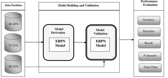
Overall process of model is depicted in Figure 1.This process can be viewed in three different stages: Data partition, model building and validation and performance evaluation. Each of these stages are explained below:

2.1 Data Set

Fig 1: Framework for E-m

ail data classification

Fig 1: Framework for E-mail data classification

2.2 Error Back Propagation Network

(EBPN)

A neural network [3] is a set of connected input/output units in which each connection has a weight associated with it. During the learning phase, the network learns by adjusting the weights so as to able to predict the correct class label of the input tuples. Artificial Neural Network learning is also referred to as connectionist learning due to the connections layers units. Error Back Propagation Network (EBPN) is a kind of feed forward network (FFN) in which Error Back Propagation Algorithm (EBPA) is used for training which one of the most is

widely used training algorithm where training is perform in two phases (i) Forward phase: In this phase input is presented and output is calculated based on activation function and finally error is calculated at outer layer. (ii) Backward phase: In this phase error is send back to the inner layers to adjust the weights. A typical architecture of EBPN with one hidden layer is shown in figure 2.In this network samples are presented one by one to derive the models and it is classified either as spam e-mail or non-spam e-mail.

Fig 2: An Artificial neural network for Spam-E-mail classification Model

Derivation

75-25%

EBPN

Model

Model Validation

Data Partition

Accuracy

Precision

Recall

F-measure

Gain Chart 60-40%

80-20%

EBPN

Model

. .

Spam

Non-Spam .

.

Spam E-mail Data

Input layer

Hidden layer

2.3 Performance Measurement

Performance of each classifier (model) can be evaluated by using some very well-known statistical measures: classification accuracy, precision, recall, and F-measure. These measures [8] are defined by true positive (TP), true negative (TN), false positive (FP) and false negative (FN) in form of confusion matrix. Where TP refers number of positive samples which is correctly classified by classifier, TN is number of negative samples classified correctly by the classifier, similarly FP are number of negative samples that is incorrectly classified (sample of class spam for which the classifier predicted non-spam) where as FN are the number of positive sample that is incorrectly classified (sample of class non-spam for which classifier predicted spam).

If the total number of samples are N then statistical performance measures can be expressed as below:

Classification Accuracy: Classification accuracy of the classifier is the proportion of instances which are correctly classified.

Classification accuracy = (TP+TN)/N … (1)

Precision: Precision is the rate of instances classified correctly among the result of classifier. Precision =TP/ (TP+FP) … (2)

Recall: Recall is the rate of correct classified instances among them to be classified correctly.

Recall =TP/ (TP +FN) … (3)

F-measure: and F-measure is the harmonic mean of precision and recall.

F -measure … (4)

Table 1: Confusion matrix for positive and negative samples

Gain Chart [11] is another way to check the classifier which plots the values in the gains (%) column from the table. Gains are defined as the proportion of hits in each increment relative to the total number of hits in the tree, using the equation:

(Hits in increment / total number of hits) x 100%

Cumulative gains charts always start at 0% and end at 100% as we go from left to right. For a good model, the gains chart will rise steeply toward 100% and then level off. A model that provides no information will follow the diagonal from lower left to upper right.

3. FEATURE SELECTION

Feature selection [9] is an optimization process in which one tries to find the best feature subset, from the fixed set of the original features, according to a given processing goal and feature selection criteria, without feature transformation or construction. The existing feature selection methods depending on feature

selection criterion used two main streams: first are open-loop methods and second are closed-loop methods.

The open-loop methods, also called the filter, present bias, or the front end methods, are based mostly on selecting features using between-class separability criteria. These methods do not consider the effect of the selected features on the entire processing algorithm’s performance. Instead, they select these features for which the resulting reduced data set has maximal between–class separability,defined usually based on between– class and between-class covariances (or scatter matrices) and their combination. Ignoring the effect of the selected feature subset on the performance of classifier is a weak side of the open-loop methods. The closed-loop methods called also the wrapper, performance bias, or classifier feedback methods, are based on the feature selection using a classifier performance as criterion of feature subset selection. The closed-loop methods will generally provide a better selection of subset, since they based on the unlimited goal of optimal feature selection, which is providing the best classification.

In this paper we have used feature selection technique with feature ranking. The simple feature selection procedure is based on evaluation of classification power of individual features, it then ranks such evaluated features, and eventually selects the first best m features. A criteria applied to an individual feature could be either open-loop type or closed-loop type. This also relies on an assumption that the final selection criterion can be expressed as a sum or product of the criteria evaluated for each feature independently. We can expect that a single feature alone have a low classification power. However, this feature when put together with others may exhibit substantial classification power.

4. EXPERIMENTAL WORKS AND

RESULTS

As explained above e-mail data set is divided into three different partitions each having training and testing data. Partition size of data plays very important role to derive a robust classification model. The three different partitions are as below:

Partition 1: 60-40%, Partition 2: 75-25%, Partition 3: 80-20%.

EBPN may trap on local minima due to various reasons , a rough value of learning rate (α) is one of them. Both higher value and a lower value of learning rate may create problem of local minima and network paralysis, therefore to obtain best classification model with high accuracy a suitable value of learning rates is required which lies between 0 and 1.To simulate our work we have considered α=0.2,0.3,0.4,0.5,0.6,0.7,0.8 and 0.9 along with different partitions. Simulated results in case of different learning rate and different partitions for both training and testing is shown in table 2, from this table it is clear that EBPN is performing well in case of α=0.9 for partition3, however there is very slight variation in accuracy from one case to another, but at the same time it is also true that training-testing size and suitable value of learning rate (α) plays import role in terms of accuracy of model. The highest accuracy calculated using equation 1 is 98.38% as highlighted for testing in table 2.

Among the various model tested we have obtained highest accuracy in case of EBPN with learning rate 0.9 using partition 3. We select this model to apply feature selection technique on it. Due to large number of features (57 features) we need to identify relevant features to retain and identify irrelevant features to be eliminated. Simple feature selection subsets can be obtained using ranking based feature selection technique. In this ranking Actual Vs.

Predicted Positive Negative

Positive True Positive (TP) False Negative (FN)

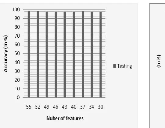
based feature selection, out of n features select subsets m features where m < n. We have obtained feature subsets with 55, 52,49,46,43,40,37,34 and 30 selected features as shown in table 3 and obtained highest accuracy of 98.49% in case of 52 features on testing data . The same is also depicted in figure 4 in form of bar chart, we can also see accuracy of an EBPN classifier with different feature subset. Accuracy obtained in case of 52 feature subset is highest among all, even it is higher than the accuracy of

data set with all features, hence it is clear that, there are some irrelevant features available in the spam e-mail data set which must be discarded to speed up performance of the classifier. An EBPN trained and tested with data set having 52 features is finally selected for spam filtering.

Table 2: Classification accuracy

(a) Accuracy with 60-40% partition

(c) Accuracy with 80-20% partition

Fig 3: Comparative chart of training and testing accuracy with different learning rate and with different

partition

(b) Accuracy with 75-25% partition

Table 3: Feature selection of best model

Number of features Testing Accuracy (%)

55 98.38

52 98.49

49 97.74

46 97.84

43 97.84

40 97.95

37 98.06

34 97.74

30 97.84

Learning Rate( α)

Partition1 Partition2 Partition3

Training Testing Training Testing Training Testing

0.9 98.41 98.15 98.44 97.73 98.56 98.38

0.8 98.66 98.26 98.47 97.73 98.37 98.28

0.7 98.52 97.88 98.50 97.55 98.04 97.95

0.6 98.48 98.21 98.61 98.08 98.45 98.17

0.5 98.04 97.66 98.18 97.21 98.28 98.28

0.4 98.37 97.99 98.52 97.82 98.42 98.28

0.3 98.44 97.83 98.64 98.08 98.26 98.17

Fig 4: Accuracy of the best model with feature selection

A confusion matrix for the best model (A model with α=0.9 for partition 3 and 52 feature subset) is shown in table 4, from this table it is clear that there is misclassification of data by the model, say for example: in case of non spam e-mail samples we correctly classified 535 emails while in case of spam e-mail 379 e-mail are classified correctly ,there are misclassification of 5 samples and 9 samples of non-spam and spam category of data respectively. In order to check the robustness of EBPN based models, other error measures: precision, recall and F-measure have also been calculated using equation 2, 3 and 4 respectively and shown in table 5.It is clear that all the measures are near or above 99% which shows the classification ability of the model. A corresponding bar chart is also shown in figure 5.Figure 6 shows the gain chart of the model which is appropriate in the term of efficiency of the model.

Table 4: Confusion matrix of best model

Table 5: Various performance measures

Fig 5: Various performance measures for best model

Fig 6: Gain chart of best model

5. CONCLUSION

Spam e-mails have become a big problem in the Internet world and it creates several problems for mail users. These spam e-mails may come from fake institutions which pretend to be authentic institutions like bank, government organizations or some others financial institutions. To curb this problem we need to have a robust e-mail system capable of classifying e-mails into spam e-mails and genuine e-mails.

In this study artificial neural network based EBPN technique is explored with different partitions of e-mail data set with different learning rate. A suitable EBPN model with highest testing accuracy of 98.38% is obtained using 80-20% ratio of training and testing samples with learning rate 0.9. Further rank based feature selection technique is applied for above model with various feature subsets and it is observed that model has obtained highest accuracy of 98.49% on testing data with 52 features which is higher than original EBPN model with set of 57 features . In future other ANN models like RBFN and SOM can be explored and can be used to derive hybrid model to achieve higher accuracy.

Actual Vs.

Predicted Testing dataset

Non-Spam Spam

Non-Spam 535 5

Spam 9 379

Performance measures _{Testing dataset}

Accuracy 98.49%

Precision 98.34%

Recall 99.07%

6. REFERENCES

[1]. El-Sayed M. El-Alfy et al., “Using GMDH-based networks for improved spam detection and email feature analysis”, Applied soft computing, vol. 11, pp. 477-488, 2011. [2]. Ismaila Idris, “E-mail spam classification with ANN and

Negative selection algorithms”, International Journal of Computer Science & Communication Networks, Vol. 1(3), pp 227-231, 2011.

[3]. Jiawei Han and Micheline Kamber, “Data Mining Concepts and Techniques “, Morgan Kaufmann, San Francisco, Second Edition, 2006.

[4]. Omar Saad et al. , “A Survey of machine learning Techniques for spam filtering”, IJCSNS International Journal of Computer Science and Network Security, vol. 12 No.2,2012.

[5]. W. A. Awad, “Machine Learning methods for email classification”, International Journal of Computer Applications vol. 16– No.1, pp. 0975 – 8887, 2011.

[6]. Hota H.S. et al. ,”Data mining techniques and its ensemble model applied for classification of e-mail data”, proceeding of review of business and technology research in International conference EPPICTM ,vol. 5 ,No. 1, ,pp. 473-479,2012.

[7]. Hota H.S. et al.,”E-mail and its security: A modern way of teaching and research”, proceeding of International conference on Innovation and Research in technology for Sustainable Development (ICIRT) pp. 168-170, ISBN 978-93-82338-21-5,2012.

[8]. Lei SHI, et al.,”Spam E-mail classification using decision tree ensemble”, Journal of Computational Information Systems, vol 8,N0.3 pp. 949-956,2012.

[9]. K., J., Cios et al., “Data mining methods for knowledge discovery”, 3rd

printing, kluwer academic publishers, (USA),2000.

[10]. UCI Machine Learning Repository of machine learning databases (2010). University of California, school of Information and Computer Science, Irvine. C.A.

http://archive.ics.uci.edu/ml/datasets/Spambase, August

2012.

[11]. SPSS Clementine help file http//www.spss.com last accessed on Oct 2012.