Characteristic function approach to the sum of stochastic variables

Munich Personal RePEc Archive

Characteristic function approach to the

sum of stochastic variables

Figueiredo, Annibal and Gleria, Iram and Matsushita, Raul

and Da Silva, Sergio

Federal University of Santa Catarina

2006

Online at

https://mpra.ub.uni-muenchen.de/1984/

Characteristic function approach to the

sum of stochastic variables

Annibal Figueiredo

a_{, Iram Gleria}b*_{, Raul Matsushita}c_{, Sergio Da Silva}d

a

Department of Physics, University of Brasilia, 70910-900 Brasilia DF, Brazil

b

Department of Physics, Federal University of Alagoas, 57072-970 Maceio AL, Brazil

c

Department of Statistics, University of Brasilia, 70910-900 Brasilia DF, Brazil

d

Department of Economics, Federal University of Santa Catarina, 88049-970 Florianopolis SC, Brazil

Abstract

This paper puts forward a technique based on the characteristic function to tackle the problem of the sum of stochastic variables. We consider independent processes whose reduced variables are identically distributed, including those that violate the conditions for the central limit theorem to hold. We also consider processes that are correlated and analyze the role of nonlinear autocorrelations in their convergence to a Gaussian. We demonstrate that nonidentity in independent processes is related to autocorrelations in nonindependent processes. We exemplify our approach with data from foreign exchange rates.

Keywords: Central limit theorem; characteristic function; reduced variables; autocorrelation

1 Introduction

The problem of the limit of sums of random variables attracted great interest in the second

half of the 19th century and the first one of the 20th century. At the time mathematicians

extending Bernoulli’s and Moivre-Laplace’s theorems were also pioneering the modern theory of the sum of random variables.

Hot topics in the research agenda included searching for general conditions under which the sum of random variables converges to a Gaussian. Liapunoff, Lindberg, and Levy are among those who contributed to clarify the problem.

Liapunoff suggested his statistical moments approach (Liapunoff, 1900); Lindberg came up with his convolution technique (Lindberg, 1922), and Levy focused on the classic approach to the characteristic function (CF) (Levy, 1924, 1929).

Levy not only analyzed the convergence of sums of random variables but also extended the classic approach to consider infinite first and second moments. He also examined the role of stable distributions in characterizing the limits of sums of random variables. In particular, he put forward ‘extraordinary laws’ to show how his stable distributions (today’s Levy-stable distributions) play a role similar to that of the Gaussian when the second moment is infinite.

* Corresponding author.

Levy’s central limit theorem settles the conditions under which sums of random variables converge to a Levy-stable distribution. Here the Gaussian collapses to a special case of the entire family of Levy-stable distributions.

Roughly Levy’s approach can be seen as an application of Kolmogorov’s triangular scheme (Gnedenko and Kolmogorov, 1954), which encompasses previous results in terms of limit theorems. In what follows we will discuss the triangular scheme in greater detail since it helps to put our results in this paper into perspective.

A triangular arrangement of random variables takes the form

( ) ( ) ( ) ( ) 1 2

( , ,..., ); 1, 2,...,

n n n n

n

x x x n

= = ∞

X (1)

where the random variables x_i(n)(i=1,…,n) are defined in the same probability space so as to satisfy two properties. (1) Random variables x₁(n),…,x(_nn) are independent for every n,

and (2) for all ε∈R, it holds true that

{

( )

}

1

lim sup 1 _i n ( ) 0

n→ ∞ _{≤ ≤i n} − f ε = , where

) (n i

f is the CF

of x_i(n). These are the conditions of independence and infinitesimality respectively. We consider sum sequence

( ) ( ) 1 ...

n n

n n n

S =x + +x +a (2)

that is related to the nth row of the triangular arrangement in Eq. (1) (the a_n is a constant of fine tuning).

Our problem is to examine the limit of the distribution of S_n assuming the

probability distributions of variables (n)

i

x (i=1,…,n) to be known. If the limit of the

distribution of S_n does exist, we are able to tackle the problem of its slow convergence.

Here our two main tasks are to characterize the class of each possible limit of sums in Eq.

(2), and to devise convergence criteria for sum S_n as a function of the properties of the

distributions of x_i(n) (i =1,…,n).

Kolmogorov hypothesized that the class of possible limits of S_n matches the class

of Finetti’s (Finetti, 1929) infinitely divisible distributions. Kolmogorov’s student Bavly

(Bavly, 1936) confirmed the hypothesis to the case where second moments of x_i(n)

(i=1,…,n) are finite. And a broader proof was presented soon afterwards (Khintchine,

1938). (A comprehensive discussion can be found elsewhere (Zolotarev, 1990)). And Gnedenko and Kolmogorov (Gnedenko and Kolmogorov, 1954), and Levy (Levy, 1937) are primers on the classic theory of the sum of random variables.)

Another key question is to address the conditions for sum S_n to converge to a

Levy-stable distribution under the independence and infinitesimality conditions (Feller, 1935), (Feller, 1937). Lindberg-Feller condition is currently known as the central limit theorem. Yet this condition is valid only for sums satisfying independence and infinitesimality.

independence and infinitesimality. He showed convergence of S_n to a Gaussian without relying on infinitesimality (Levy, 1937). Unfortunately this finding made negligible impact on literature.

From the mid-1960s to the 1970s and 1980s, Russian mathematician Zolotarev made a significant breakthrough (Zolotarev, 1965, 1997). He examined convergence of the sum of random variables without relying on the classic assumptions. Zolotarev dubbed ‘non-classic’ the limit theorems lacking the independence and infinitesimality conditions. His work gave rise to a broader theory of the existence of limits in sums of random variables. The infinitesimality condition was left out and asymptotic independence was assumed (Zolotarev, 1990). One key result is his Theorem 5 (at page 131) showing necessary and sufficient conditions for convergence of sums of random variables.

Our own work in this paper elaborates further on such a non-classic framework. Yet our interest goes beyond theory in that we also devise applications to the statistical analysis of actual time series.

Our previous work is motivated by Mantegna and Stanley’s (Mantegna and Stanley, 1994, 1995). We show the general approach of the CF to the sum of random variables to be useful to tracking convergence in time series of financial returns (Figueiredo et al., 2003).

And also how correlations are key in curbing convergence to the Gaussian (Figueiredo et

al., 2004). We put forward that Mantegna and Stanley’s truncated Levy flights can be

explained by linear and nonlinear autocorrelation in data. Moreover we show how departures from infinitesimality are related to financial volatility in that they can explain lack of convergence to the Gaussian (Figueiredo et al., 2005).

In particular, our aim in this paper is to develop a general technique to approaching convergence without relying on independence and infinitesimality. Our technique belongs to the class of non-classic methods that are based on the analysis of empirical CFs

(Feuerverger, 1977, 1981). An important role is played by a function ( )ω z univocally

associated with a reduced distribution, which is the canonical form of Levy’s CF (Levy, 1924). We confine ourselves to the analysis of processes with finite second moment, thereby rendering it useful for applications.

This paper departs from Zolotarev’s in two ways. (1) We propose theorems without relying on infinitesimality (like him); the latter is replaced with volatility change in the sum. (2) We put forward general results that alow one to gauge the effect of autocorrelations in convergence without imposing any specific functional form to the CF.

Indeed we are able to reckon the part of function ( )ω z that is exclusively related to the

autocorrelations.

Employing the canonical form of the CF allows one to get fruitful results based solely on classic theory. And using function ( )ω z enables one to devise statistical gauges of the distance of a given distribution to the Gaussian. What is more, the convergence rate of an actual process can be measured and then compared to that of an independent and identically distributed (IID) one.

2 Existence of limits in the sum of random variables

consider these variables to be sorted such that mi( )n ≥ m( )jn for i > j and ,i j =1, ...,n .

We define the reduced variable as _{( )}

) ( ) ( ) (

n i

n i n i n i

m x

x = −µ and can then rewrite the sum in Eq. (2)

as

( ) ( ) 1

n

n n n n i i

i

S a m x

=

− =

∑

₍₃₎

where an now stands for the mean of Sn .

One of the most important issues concerning the sequences of sums given by Eq. (3)

is related to convergence of the probability distribution of S_n as n → ∞ . To answer this

question we apply the CF method as developed by Levy in his 1924 seminal work (Levy, 1924). The method consists in calculating the CF of the reduced variable

n n

n

n

S a S

M

−

= (4)

where M_n is standard deviation of S_n. Assuming variables ( )n

i

x to be statistically

independent one has

2 ( ) 2 1

( )

n n

n i

i

M m

=

=

∑

(5)

For a reduced random real variable (i.e. one with zero mean and unit variance), its CF is (Levy, 1922)

( )

2

1 ( ) 2

( ) , ( ) ( ) ( ), (0) 0

z z Iz

R I

z e e ω z z I z

ψ = 〈 〉 = − + ω =ω + ω ω =

Denoting ( )ψ z =ψ_R( )z +Iψ_I( )z yields

2

2 2

2 ln 2

, arctan I, R

R I

z

z z

ψ ψ ψ

ω ω

ψ ψ

 

− −

= = _− _

 

For Gaussian distributions one has ω(z)=0 for all z∈R. Function ( )ω z uniquely

determines the distribution function of a given reduced variable. The CF of reduced variable x_i( )n is

( )

2 ( )

1 ( )

( ) ₂

( )

n i

z z n

i z e

ω

ψ = − + (6)

( )

2

1 ( ) 2

( ) n

z z

n z e

− +Ω

Ψ = (7)

where

∑

=                 = Ω n j n n j n j n n j n z M m M m z 1 ) ( ) ( ) ( )

( ω (8)

In the framework of the classic central limit theorem one condition for the CF in (7) to

converge to a Gaussian (lim _n

( )

0

n→∞Ω z = ) is precisely the infinitesimality hypothesis

(referred to in Section 1). It states that

{ }

( ) 1

max ,

0

lim _in

n i n n

n

n→∞_M = µ = ≤≤ m

µ

Yet infinitesimality does not hold for m_i( )n . As a consequence, if we wish to track

asymptotical behaviour, we need to develop tools capable of evaluating limit distributions for sums S_n without relying on infinitesimality.

As observed, Zolotarev and co-workers (Zolotarev, 1990) established the conditions

for convergence of sum S_n in a non-classic limit theorem. Inspired by the works of

Zolotarev, and using Levy’s CF formalism, we state a theorem as follows.

Theorem 1. Consider the sum in Eq. (2) and assume

(1) ( ) lim n i i n n m M λ →∞

= to exist for all i∈N. And

(2) _i( ) lim _i( )n

( )

n

z z

ω ω

→∞

= to exist for all i∈N.

Thus _{lim n}( ) ( )

n

z z

→∞

Ψ ≡ Ψ too exists and can be written as

2

(1 ( )) 2

( ) z

z

z e− +Ω

Ψ = (9)

Such a limit defines the limit distribution’s CF for S_n. And function Ω( )z is given by

1

( ) _{i i}( _i )

i

z λ ω λz

∞

=

Proof. Define the sequence of random variables y y₁, ₂,...,y_n such that (1) the means of y y₁, ₂,...,y_n are zero,

(2) the standard deviation of y_i is λ_i, and

(3) reduced variables y_i/λ_i have a CF given by ( )

2

1 ( ) 2

( ) i

i

z z

z e ω

φ = − +

Then let us consider the sum y₁+y₂+ +... y_n =Y_n, and its reduced variable

1 2

, ...

n

n n n

n

Y

Y σ λ λ λ

σ

= = + + + . It is clear that lim _n 1

n→∞σ = . According to a Kolmogorov`s

(Kolmogorov, 1921) theorem, variable Y_n converges in probability to a finite value. Its CF

is given by (9) and (10). Thus the series in (10) converges to all z, and is continuous in the

neighborhood of the origin. According hypothesis (1) and (2) the function Ω_n(z), given by

Eq. (8), converges to the function given in Eq. (10), then we conclude that sequence in Eq. (7) converges for all z and its limit is continuous around the origin. Thus, according to

Levy’s continuity theorem, we conclude that the distribution of S_n M_n converges to a

well-defined limit distribution.

Now we move on to define an identically distributed reduced process (IDRP) as one in which ωi( )n( )z =ω( ),z i=1,...,n. In this case the stochastic variables

) (n i

x have the same

reduced distribution.

Since the )(n)(_z

i

ω s are the same, then hypothesis 2 of Theorem 1 holds. We assume

hypothesis 1 to hold as well. Considering Eq. (6) yields

2

(1 ( ))

( ) ₂

( ) ( )

z z n

i z e z

ω

ψ = − + ≡ψ (11)

If ψ( )z is analytic, then all statistical moments of the distribution are finite. As a result, one gets Taylor expansion

( )

2 1 2 3 3 3 4 4 4 ( )

( ) 1 ...,

2! 3! 4!

p n

p i

z I z I µ z I µ z X

ψ = + + + + µ = 〈 〉 (12)

Function

ω

( )z =

ω

_R( )z +I

ω

_I( )z in Eq. (11) can also be expanded in series to produce

2 4 2

2 4 2

1 3 2 1

1 3 2 1

( ) ... ...

( ) ... ...

p

R p

p

I p

z K z K z K z

z K z K z K z

ω

ω

−

−

= + + + +

= + + + + (13)

. K , K , K , K 6 4 2 3 4 5 3 3 4 2 3 1 360 1 24 1 36 1 12 1 60 1 6 1 12 1 4 1 3 1 µ µ µ µ µ µ µ + − − = + − = − = − = (14)

Now we expand function Ω( )z = Ω_R( )z + ΩI _I( )z in Eq. (10) in series

2 4 2

2 4 2

3 2 1

1 3 2 1

( ) ... ( ) ... p R p p I p

z L z L z L z

z L z L z L ₋z −

Ω = + + +

Ω = + + + (15)

So

2 2

1 1

( ) ( ), ( ) ( )

R i R i I i I i

n n

z λ ω λ z z λ ω λ z

∞ ∞

= =

Ω =

∑

Ω =

∑

(16)

Substituting Eq. (13) in Eq. (16) and comparing the output with Eq. (15) produce

2 1

, lim , 1

p i

p p i i

n _n

n

m

L K p

M λ λ ∞ + → ∞ =

=

∑

= ≥ (17)

Thus one gets an expression for the CF of IDRPs with analytical distributions of x_i(n).

What if this condition is not fulfilled? Here x_i(n) will have infinite moments. To examine this case we first show that the CF in Eq. (11) can be expanded in terms of the finite moments of the distribution.

3 Another theorem on the existence of limits to the sum of random variables

Now we consider that a variable x_i(n) has finite moments up to order 4. Its kurtosis will be denoted by K_i( )n and its skewness by S_i( )n . The reduced variable’s CF satisfies

2 ( )

(1 ( ))

( )_{( )} 2 _{, (0) 0} n

i

z z n

i z e i

ω

ψ = − + ω = (18)

and

( ) ( )

( ) 2 ( )

( ) ( )

3 12

n n

n i i n

i i

S K

z I z z z

ω = − − +ρ (19)

( )

( ) 2

2

( )

( ) ( ), 0, 0

n

n i

i

z

z O z z

z

ρ

ρ = → →

The CF of reduced variable S_n can be obtained using Ω_n( )z . From Eq. (19) we can write

( )

2 ( )

4 3 ( )

( ) 2 ( )

4 3 2 ( )

1 1 1

1 1

12 3

n _n

n n n

i

n i n i i

n i i i n

i n i n i n n

m

m m m

K z I S z z

M M M ρ M

= = =

     

Ω = − _{ } − _{ } + _{ }



∑

 

∑



∑

  (20)

At this point we make the samehypotheses 1 and 2 of Theorem 1, apart from the fact that

now we replace functions ω_i(n)(z) with functions ρ_i(n)(z) and consider an extra hypothesis as follows.

(3) Both series

4 4 1 i i i n m K M ∞ =    



∑

 and

3 3 1 i i i n m S M ∞ =    



∑

 converge.

Thus we can state another theorem.

Theorem 2. If the sum of random variables in Eq. (2) is such that hypotheses 1−3 hold, then there exists a distribution F (associated with the reduced variable) that is the limit of

the process as n→∞.

4 Limits to the sum of random variables when the variance follows a formation law

Now we reckon functions Ω(z) and Ω_n(z) to processes following a formation law in the

second moment. We consider two cases in IDRPs, namely

(1) Exponential law:m_i( )n ≡m_i = AeBi,A>0,B∈ ℜ, and (2) Power law: m_i( )n ≡m_i = AiB,A>0,B∈ ℜ.

4.1 Analysis of the exponential law

To fully understand lim i

n n m M →∞    

 , we need to evaluate Mn. For

Bi i

m =Ae ,

2 2 1 2 0 B i i m e r m

+ _{= ≡ > (21)}

holds. Here Mn is given by

(

)

2 2 2 1

1 1 ...

n n

Taking the sum in Eq. (22) yields

2 2 1

1 1

n

n

r

M m

r

 − 

= _{ }

−

  (23)

We assess two possibilities, namely

(1) lim n (1 )1/ 2 0

n

n

r M

µ

→∞

 

= − >

 

  , if 0<r <1

and

(2)

1 2

1

lim n

n _n

r

M r

µ

→∞

 ₌ −    _ _

  , if r >1

where n max

{

i, 1,...,

}

i

m i n

µ = = . Thus according to Theorem 1, sum variable S_n presents a

limit distribution function that fails to be Gaussian.

4.2 Analysis of the power law

Now we turn to the power law. It is appropriate to introduce function

( , ) 1 2r 3r ... r,

Z n r = + + + +n r∈ℜ (24)

We can then write

2 2 2 2

, ( , ), 2

r

i n

m = A i M =A Z n r r= B (25)

We consider the cases r< −1 and r≥ −1. Calculations (not shown) for r< −1 take account of the fact that

1

lim lim

( , ) n

n n

n

M Z n r

µ

→∞ →∞

 

=

 

  (26)

where

0

1 1

lim ( , ) ( ) lim 0, ( )

( ) n

r

n n _p

n

Z n r r r

M r p

µ

ξ ξ

ξ

∞

and ξ( r ) is Riemman’s zeta function. Thus the limit distribution fails to be Gaussian and

lim _n

n→∞M has a finite value.

For case r≥ −1, we have lim n 0

n n

M

µ

→∞ = , and the limit distribution function is

Gaussian.

4.3 Characteristic function of identically distributed reduced processes

Now we tackle the problem of determination of the CF in IDRPs. We take the case of an analytical CF. If the CF is analytic, function ( )ω z can be expanded in series as in Eqs. (13)

and (15). Considering these equations we have

2 1 p n i np p i n m L K M + =   = _{ }  

∑

. Our task is to

calculate an expression for

2 1 p n i i n m M + =      

∑

.

We again illustrate our case with exponential and power laws. As for the exponential law one has

2

1 2

2 1

2 2

1 ( )

p i p B i i p i m

m m r r e r R

m + − + +   = = →_{ } = =

  (28)

Thus sum m₁p+m₂p+ +... m_np is geometric and accordingly

2

1 2 1

1 ...

1 n p

p p p p

n

p

R

m m m m

R

+  − 

+ + + = _ _

−

  (29)

Using Eq. (23) for Mn yields

2 2 2 1 1 1 p n p p n r M m r + +  −  = _{ } −

  (30)

And from Eqs. (29) and (30) one gets

(

)

(

)

2 2 2 2 2 2 2 2 1 1

, 0 1

1 1

p

p _n

np p _{p p}

n

r r

L K r

r r + + + +   − _ − _  

= < <

 

− −

 

 

and

(

)

(

1

)

1

1 1 1 2 2 2 2 2 2 2 2 > −         −         − − = + + + + r , r r r r K L p n p n p p p

np (32)

As n→∞ function Ω( )z becomes

( ) p p

p p

i even i odd

z L z I L z

= =

Ω = ∑ + ∑

where

2 2

2 2

2 2

2 2

(1 ) ( 1)

lim , 0 1, lim , 1

1 1

p p

p _n np p p p _n np p p

r r

L L K r L L K r

r r

+ +

+ +

→∞ →∞

− −

= = < < = = >

   

− −

   

   

(33)

As for the power law, it can be shown that

2

2 2 2 2 2 2

1

2

( , ) , ... ,

2 p

p p p p p

n n

p

M A Z n r m m A Z n r

+

+ ₌ + + _{+ +} + ₌ +  + 

 

  (34)

and then one gets

2 2 2 , 2 ( , )

np p p

p

Z n r

L K

Z n r

+

+

 

 

 

= (35)

Thus as n→∞ function Ω( )z is either

2 2,

2 2

lim , 1

p np p _p

n

p r

L L K r

r ξ ξ + →∞  +     

= = < −

 

 

 

(36)

or

lim 0 ( ) 0, 1

p np

n

L L z r

→∞

In the latter case the process will reach the Gaussian regime. For the distinct processes defined by r =2B >−1 there will be different ‘convergence speeds’, as measured by L_np

in Eq. (35).

Now we will examine the asymptotic behavior of both M_n and the terms in the

expansion of Ω_n. Our approach relies heavily on analysis of Z(n,r). It can be shown that

1

( , ) ( ) 1

( , ) log 1

( , ) 1

1 r

Z n r r r

Z n r (n) r

n

Z n r r

r

ξ

+

→ < −

→ = −

→ > − +

(38)

As for the analytical IDRPs with second moment m_i =m₁ir/2, we consider results

for five distinct values of r.

(1) For 1r <− , using Eqs. (35) and (38) one can show that a process converges to a

non-Gaussian distribution where variance M_n and the asymptotic terms in the series of

n

Ω are

( )

(

(

)

)

( )

( )

1 / 2

1 2 / 2

2 /

, ,

n np p p

p r

M m r L K p N

r ξ ξ ξ − + +

→ → ∈ (39)

(2) For 1r =− , a process converges to a Gaussian distribution where the variance

and the asymptotic terms in the series of Ω_n are

(

)

1 / 2

(

(

)

)

₁

1 log , 2 / 2 (log ) ,

n np p

M → m n L → K ξ p+ n − p∈N (40)

(3) For −1<r<0, a process converges to a Gaussian where the variance and the

asymptotic terms in the series of Ω_n are

(

)

( )

(

)

1 / 2 1

1 / 2

( 2 ) / 2 / 2

( 2 ) / 2

( 2 )( 1) / 2

( 2 ) / 2

( 2 )( 1) / 2

1

2( 1)

, ( 2) / 2 1

2 ( 2)

log

( 1) , ( 2) / 2 1

( 2) / 2

( 1) , ( 2) / 2 1

r n p p np p p

np p p r

p

np p p r

m

M n

r

r

L K n p r

p r

n

L K r p r

n

p r

L K r p r

n ξ + + − + + + + + + → + +

→ + > −

+ +

→ + + = −

+

→ + + < −

(41)

(4) For r =0 (IID process) the second moment is the same for all i, i.e.

1

m m i → _i =

∀ . The process converges to a Gaussian with the variance and asymptotic

terms in the series of Ω_n given by

1 / 2 / 2

1 , ,

p

n np p

M → m n L → K n− p∈ N (42)

(5) For r >0, one has

(

)

( )

( 2 ) / 2

1 / 2 / 2

1 _, 2( 1) _,

1 2 ( 2)

p

r p

n np p

m r

M n L K n p N

r p r

+

+ + −

→ → ∈

+ + + (43)

At this point some remarks are worthwhile. As for r >−1 the cumulative standard

deviation M_n is governed by power law n(r+1)/2 as n→∞. And a logarithm law holds for 1

− =

r . The process then bifurcates into two ones, namely (1) convergence to a Gaussian

(r >−1), and (2) no convergence (r <−1). In the latter situation the second moment has a

saturation value at 1 / 2

1 ( )

m ξ r .

As for the power laws in r≥0, L_np (which defines the series for Ω_n( )z ) shows an

asymptotic decay with same power law n−p/2. This process thus converges at the same

pace to the Gaussian regime as n approaches infinity. But the process can show distinct

transient behavior at the onset of aggregation. A large transient phase means a slow

convergence, suggesting that Ω_n( )z varies sluggishly. This kind of behavior can be

observed in truncated Lévy flights (TLFs) (Mantegna and Stanley, 1995).

4.4 A class of nonidentically distributed processes

Now we consider a class of stochastic processes with finite fourth moment. We assume every ( )n _{( )}

i z

ω to be distinct for alternative i. If the fourth moment is finite one has

( ) 2

( ) ( ) ( )

12 3

n i i

i i

K S

z z z I z z

ω =ω = − − +ρ (44)

where ∀ ⇒i ρ_i( )z =o z( 2), i.e. i( )₂z 0

z

ρ _→

when z→0. The power laws we take are

/ 2 3 / 2 2

1 , 1 , 1 , , , , 1, 1 0

r y x

i i i

m =m i S =S i K =K i r x y∈ℜ S K ≥ (45)

In such cases

2 2

( )

12 3

n n

n

K S

z I z o z

where

3 4

3 4

1 1

,

n n

i i

n i n i

i n i n

m m

S S K K

M M

= =

   

=_{ } =_{ }



∑

 

∑

 (47)

Employing Eqs. (21) and (36) yields

(

)

(

)

1/ 2

1 1 3/ 2 1 2

, 3( ) / 2 , 2( )

( , ) , ,

( , ) ( , )

n n n

Z n r y Z n r x

M m Z n r S S K K

Z n r Z n r

+ +

= = = (48)

The IDRP calculated in this section encompasses that of previous section, where x=0 and

0

y= . And the suggested formulas are suitable for description of a class for which

, i

m =m ∀i, i.e. an IID process where x=0,y=0, and r=0.

Now we examine the asymptotic behavior of the above processes. We take into account the standard deviation, skewness, and kurtosis, as defined in Eq. (48). We consider the evolving laws in Eq. (45) with r> −1,y>0 and x>0.

As n→∞ then

(

)

( )

1 / 2 1

1 / 2

3 / 2

( 3 1) / 2 1

2

2 1 1

1

2( 1)

2 3( )

( 1)

2( ) 1

r n

y n

x n

m

M n

r

r

S S n

r y

r

K K n

r x

+

−

−

→ +

+ →

+ +

+ →

+ +

(49)

Quantities M_n, S_n, and K_n follow power laws of distinct exponents. It is intriguing (1) that M_n depends only on r, which describes the evolution of m_i, (2) that S_n depends on y,

which shows how skewness S_i evolves over time, and (3) that K_n depends only on x,

which gives the evolution of kurtosis K_i.

Note that for 0< y<1/3 one has S_n →0 as n→∞. If y =1/3 then the skewness approaches a finite value and the limit distribution will fail to be Gaussian. For

3 1/

y > one has S_n →∞ as n→∞, i.e. a limit process at an infinite distance from the Gaussian.

A similar analysis can be delivered to the kurtosis. As , n→∞

0 1/ 2 0

1/ 2 1/ 2

n

n

n

x K

x K C

x K

< < → →

= → →

> → → ∞

After a threshold value at bifurcation point ½, the third and fourth moments diverge. The bifurcation parameters are then x = 1/2and y = 1/3.

4.5 Probability of return to the origin and scaling properties of statistical moments

Now we sketch an explanation for asymptotic laws in the ‘probability of return to the origin’ of TLFs (Mantegna and Stanley, 1995). First we introduce the concept of asymptotic Ω-stability.

Definition 1. There exists an n₀ such that, for all n>n₀, function Ω_n is nearly constant.

The notion captures the idea of a process whose CF approaches a threshold. This is equivalent to Ω_n( )z = Ω( ),z ∀ >n n₀. Thus P_n(0) becomes

( )

2

1 1 ( ) 2

1 constant

(0) z z

n

n n

P e dz

M M

∞ _{− +Ω}

−∞

=

_∫

= (51)

Once we have learned the asymptotic laws governing M_n (from the cases studied here), the

asymptotic laws for P_n(0) end up known. For the exponential law one has

(

)

(

)

1/ 2 1

1/ 2 1

1

(0) for 1,

1

(0) for 1

n

n n

C r

P r

m

C r

P e r

m

−

−

= <

−

= >

(52)

And for the power law it holds that

( )

1

1/ 2 1

1/ 2

(1 ) / 2 1

(0) constant, for 1

(0) for 1

(log )

(1 ) 1

(0) for 1

n

n

n r

C

P r

m r

C

P r

m n

C r

P r

m n

ξ

+

= = < −

= = −

+

= > −

(53)

1/ 1/ 2

1/ (1 ) / 2 1

constant (0)

(1 ) 2

, , 1

1 n

n

r

D P

M n

C r

D n n r

m r

α

α + _α

= = ⇒

+

= = ⇒ = > −

+

(54)

i.e. 0α > . If −1<r <0 then 2<α <∞. If r =0 then α =2. And if r >0 then 2

0<α < . The latter case is that of a TLF. The probability of return in the remaining

cases still scales with n, but surely they cannot converge to the TLF.

For the asymptotic stable processes the evolution of moments 〈S_np〉 is entirely

determined by the evolution law of dispersion M_n. To see this remember that a CF of S_n

is

( )

2

2 3

1 ( )

2 3

2

3 0

( ) 1 ...,

2! 3!

z z n

I I

z e− +Ω z K z n n

Ψ = = + + + ∀ > (55)

And that the CF of S_n is

2 3

2 2 3 3

3

( ) ( ) 1 ...

2! 3!

n n n n n

I I

z M z M z M K z

Ψ = Ψ = + + + (56)

These two equations produce

2 3

2 2 3 3

( ) 1 ...,

2! 3!

p p

n n n n p n

I I

z S z S z S K M

Ψ = + 〈 〉 + 〈 〉 + 〈 〉 = (57)

Thus the evolution law of M_n fully determines other moments’ motion laws.

5 Example

This section employs some of the results in previous sections to examine a financial time

series, namely the Brazilian real–US dollar exchange rate. We take returns Z rather than

raw data as our stochastic variable, i.e. Z∆t(t)=Y(t+∆t)−Y(t) where Y(t) is a rate at day t.

Returns x_i are ranked, i.e. m₁≥m₂ ≥ ≥... m_n. We define vector Xn =

(

x x₁, ₂, ...,xn

)

and

permutation operator P such that

(

)

1, ... n

n i i

PX = x x with ( , ...,i₁ i_n) being any

permutation of (1, ..., )n . Sum variable is

(

)

1 ... n

n i i n

X =x + +x =S PX .

Then we define an event as an n-dimensional, real vector generated by the following

Definition 2. To create event E we first select vector X_n and permutation operator P,

and then build up another vector in which the k th component is randomly generated by a

number from the distribution of

x

_ik .

The event is a realization of vector X_n followed by a permutation of any of its

components. The sum of N events E _i=

(

E E_i1, _i2,...E_in

)

is defined as

1

( ) ...

i i i in

S =S E =E + +E . For N large enough, sequence S S_1,, ₂,...,S_N presents the same

distribution as that of sum variable X_n.

For series of events E E₁, ₂,...,E_N, a list of N'=nN numbers can be obtained, i.e.

1,..., n, n 1,..., 2n,..., (N 1)n 1,..., nN

u u u ₊ u u _{− +} u

 

=  

u (58)

where u₁=E₁₁,u₂ =E₁₂,...,u_n =E_1n,u_n+1=E₂₁. Eq. (58) can be thought of as an n-periodic stochastic process. If a period is known with certainty, Eq. (58) can be used to produce list

1

[U ,...,U_N]

=

U , where U₁= + +u₁ ... u U_n, ₂ =u_n+1+ +... u_2n,..., and so on. How to get the

standard deviations m_i? One is aware by the very nature of the process that they are not

ordered. Besides, it is not generally possible to evaluate the standard variation of a stochastic variable from a single measure. But such problems can still be overcome (see (Figueiredo et al. 2005).)

We then employ such a routine to the 15-minute spaced Brazilian real-US dollar

rate from year 2002 (Fig. 1). Using Eq. (58) we get list u from this set of data. The list is

made up of N′ = 6140 numbers. Then we get list U from a ‘daily’ set of data, which is

built up as follows. A ‘day’ is considered to have 20 data points from the original 15-minute series. So the process’ period is n = 20. Since N′ = nN, list Uends up with 307 numbers.

The skewness and kurtosis of the two lists are

( ) 3.0653, ( ) 114.4593

( ) 1.5288, ( ) 19.3846

Sk K

Sk K

= =

= =

u u

U U (59)

As can be seen, the hypothesis of an IID is promptly discarded because

1/ 2 1/ 2

1 1

( ) ( ) 3.0653 0.6854

20

1 1

( ) ( ) 114.4593 5.2965

20

Sk Sk

n

K K

n

= = =

= = =

U u

U u

(60)

So we evaluate whether the process above can be explained in terms of our

suggested IDRP. To apply the technique summed up in (Figueiredo et al., 2005) we take N

(

)

(

)

3 3 1 3/ 2 2 2 1 4 4 1 2 2 2 1 ...

( ) ( ) 1.3497

...

...

( ) ( ) 25.6804

... n n n n m m Sk Sk m m m m K K m m + + = = + + + + = = + + U u U u (61)

which is in good agreement with experimental data.

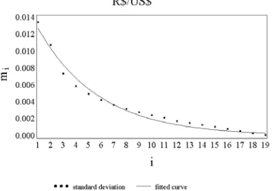
Now we examine whether there is a law governing the standard deviations in Fig. 2. First we try out exponential law m_i = Ae−Bi. Fig. 3 displays the data in Fig. 2 together with

Bi

i Ae

m = − . Using this exponential law it can be shown with some algebra that

(

)

(

_{) (}

₎

(

)

(

)

₍

(

₎

)

3 2 3 2 3/ 2 3/ 2 2 2 2 2 2 1 1 ( ) ( ) 1 ₁ 1 1

( ) ( ) , 1

1 ₁ n n n B n r r Sk Sk r _r r r

K K r e

r _r −   −   − _{ } = − ₋ − −

= = <

− ₋

U u

U u

(62)

Eq. (62) and B (Table 1) together yield

( ) 1.3086

( ) 23.9674

Sk

K

= =

U

U (63)

which is in agreement with the experimental data.

Power laws m_i = Ai−B and m_i =(A+iB)−1/C are presented in (Figueiredo et al.

2005). Table 2 sums up results. So the best fit is found with the assumption of an IDRP together with the exponential law describing second moment’s behavior.

6 Characteristic function approach to the sum of autocorrelated variables

So far only independent stochastic variables have been considered. Now we tackle the

problem of the sum of nonindependent variables (Figueiredo et al., 2004). Here we restrict

ourselves to sequence x_i( )n =x_i. We denote the moments of order p of x_i and S_n as p

ip xi

µ = 〈 〉 and p np Sn

ν = 〈 〉 respectively. The CFs of x_i and S_n are

2

2 (1 ( 2 )) / 2

( )

Ix zi i z i i z

i

z

e

e

µ ω µ

ψ

_{= 〈}

_{〉 =}

− +

(64)

2

2 (1 ( 2 )) / 2

( )

IS zn n z n n z

n

z

e

e

ν ν

− +Ω

Ψ

= 〈

〉 =

(65)

respectively.

The existence of a CF in sum variable as n→∞ is assured by Levy’s continuity

theorem. As for independent variables it holds that Ψ_n( )z =ψ₁( )...z ψ_n( )z . Yet this does not extend to autocorrelated processes where

1

( ) ( ) ( )... ( )

n z Cn zψ z ψn z

Ψ = (66)

Written ( )C z_n as

( )

2 2

2 ( )

2

( )

n n

z

C W z

n

C z

=

e

− − + , (67)

The CF in Eq. (66) then becomes

2 1 / 2 2 2 2

1

( ) ( ) / 2

( )

n

n i i i n

i

z z W z

n z e

ν µ ω µ

=

 

− _ + + _

 ∑ 

Ψ = (68)

After writing the CF of the reduced variable as

(

)

2(₁ (1)_{( )} ( 2 )_{( ) / 2}) 2

( ) / z n z n z

n z _n z ν_n e

− +Ω +Ω

Ψ = Ψ = (69)

one gets

(

)

(1)

2 2 2

1 2 1

( ) /

n

n i i i n

i n

z µ ω z µ ν

ν =

Ω =

∑

(70)

and

(

2

)

2 )

2 (

/ 1

)

( n n

n

n z =_ν W z ν

Ω (71)

Function )Ω(_n1)(z matches that for uncorrelated series, i.e. as n → ∞ it approaches zero. And term Ω(_n2)(z) is related to the existence of autocorrelations. This term gives sum

variable’s CF, which can be used to obtain its PDF as n→∞.

6.1 Autocorrelation and convergence

Now we put forward an expression for Ω(_n2)(z) containing only statistical moments.

2 3 4 4

2 3 4

( ) 1

( )

n n n n

C z

= +

C z

+

C z

+

C z

+

o z

, (72)

) (z

W_n can be extended to W_n(z)=IW_n1z+W_n2z2+o(z2). Comparing equal order terms produces

(

)

(

)

(

)

(

(

)

)

2 2 2 3 3 3

4 4 4 2 2 2

1

,

2 3!

1 1

4! 2!2!

n n n n n n

n n n n n n n

I

C C

C

ν σ ν σ

ν σ σ ν σ γ

= − − = − − = − − − + (73) where 1 1 2 2 2 2

1 1 1 1

n n n n

n i j i j

i j i i j i

x x

γ − µ µ −

= = + = = +

=

∑ ∑

=

∑ ∑

〈 〉〈 〉 and _{np ip} i

σ =

∑

µ . It can also be shown that

(

)

(

)

2

1 3 3 2 2 2 4

1 1

, 2

3 4

n n n n n n n

W = ν −σ W = ν −σ − C (74)

That renders a distribution suitable for practical purposes. First we define nonlinear autocorrelation term

(

1 1

)

1 1 2

... 1

... ... k ... k

i k i k

k n

p p

p p

k n i i i i

i i

p p p x x x x

=

〈 〉 =

∑

〈 〉 − 〈 〉 〈 〉 (75)

where p p_{1 2}...p_k are positive integers, and i₁ ≠ ≠ ≠i₂ ... i_k.

Using Eq. (69) it can be shown that Ω = Ω(2)_n I (2)_n1z+ Ω(2)_n2z2, where

( 2 ) 3 3

1 3 / 2 3 / 2

2 2

2

( 2 ) 4 4 2

2 2 2

2 2

2 2

111 3 12 1 , 3 6 1 1 1 12 4

( 1 / 12)( 1111 6 112 4 13 3 22 ) /

n n n n

n

n n

n n n n

n

n n

n n n n Rn

ν σ

ν ν

ν σ γ σ

ν ν

ν

− 〈 〉 + 〈 〉

Ω = =

 

− −

Ω = − + _ − _

 

= − 〈 〉 + 〈 〉 + 〈 〉 + 〈 〉 +

(76)

so Ω(2)_n1 and Ω(2)_n2 are functions of third- and fourth-order correlations respectively.

We conclude that, although linear autocorrelations play a key role in a distribution convergence, it is still necessary to take the nonlinear autocorrelations into account to fully characterize a process. Although that is arguably well known in literature for long, our novel technique presents formulas capturing the nonlinear terms explicitly.

6.2 Example

period from 1 April 1971 to 30 December 2005. As before, we take single returns rather than raw data.

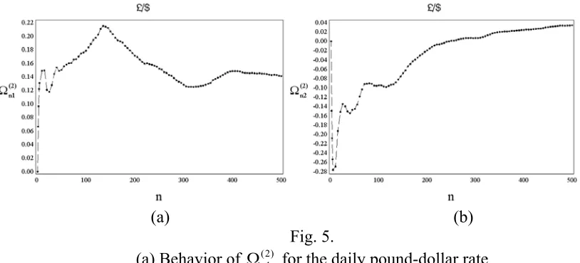
Fig. 4a displays kurtosis behavior, and Fig. 4b that of skewness. These are the

leading terms in the expansion of S_n. Curves of IID processes are shown for comparison.

The skewness is clearly bounded by real values. This limits (2)

1

n

Ω and prevents convergence

to the Gaussian regime. (Figs. 5a and 5b show Ω(_n2₁) and Ω(_n2₂) respectively.) Further details can be found elsewhere (Figueiredo et al., 2004).

7 Relating identically distributed reduced processes to autocorrelated ones

Section 5 dealt with IDRP behavior, and Section 6 examined the sum of autocorrelated variables. The purpose of this section is to relate IDRPs to autocorrelated processes.

Nonidentity of a process is entirely determined by average values µ_i1,i=1,...,N and

standard deviations µ_i2,i=1,...,N. We define a reduced random generator (RRG) with

zero mean and unit standard deviation. Every x_i obtained in an IDRP are then given by

2 1

i i r i

x = µ G +µ , where G_r is a random choice from a reduced distribution g(x) of zero

mean and unit standard deviation. Time series from an IDRP can be obtained as follows. First we pick a particular RRG, say G_r. Secondly we choose µ_i1,i=1,...,N to track how

the mean evolves over time. And finally we select µ_i2,i=1,...,N to capture standard

deviation’s time evolution.

Time series obtained from an IDRP generator can then be theoretically evaluated. We take a particular RRG derived from a truncated Cauchy (TC) distribution, i.e.

1 2

2

1 1

( ) 1

0 or

A

L x L

f x x

x L x L

 _{− ≤ ≤}

 = +

 _{< − >}



(77)

with 0L₁,L₂ > and

( )

arctan

( )

L . arctan

1

2 1 +

=

L A

Defining a random generator associated with x with distribution function f(x) is a

well-known problem. We can relate x to, say, y (which is uniformly distributed within

interval [0,1] ), and use the property of probability conservation to show that

( )

( )

( )

(

1 2 1

)

tan arctan arctan arctan

x= _ L + L _y− L (78)

Since y is uniformly distributed within [0,1], x is distributed in [−L₁,L₂] with a TC. Then

reduced variable x =

(

x−µ₁

)

µ₂ has a TC distribution. A TC RRG of α =1 can be

( )

( )

( )

(

1 2 1

)

1

2

tan arctan arctan rand() arctan

r

L L L

G µ

µ

 +  − −

 

= (79)

where rand() stands for a uniform random generator within [0,1]. Thus to fully characterize an IDRP generator we should first set µ_i1 and µ_i2 (i =1,2,…,N).

7.1 Example

We again take the time series from the daily changes of the British pound−US dollar rate to

illustrate our case. The heart of our technique is as follows. We divide such a sequence into equal, non-overlapped time periods. Then we compute the means and standard deviations of these periods. For instance, defining a p-sized period as a sequence of p days

means the series of 8780 days will have n_p periods of p days that are consecutive and

non-overlapped (n_p×p=8780). We then calculate (for each of these periods) the means and

standard deviations using the pound-dollar series.

Once p and n_p are characterized, we are ready to define IIDR random generator

( )

µi2 Gr +Aµi1,i=1, 2, 3,...,8615 (80)

where A is a real number within [0,1]. The µ_i1 and µ_i2 are given by

11 21 31 ... p1

µ =µ =µ = =µ =first-period mean,... (81)

and

12 22 32 ... p2

µ = µ = µ = = µ =first-period standard deviation,... (82)

If 0A= then we discard weekly mean’s time evolution. In this case the generator

produces a zero mean for all time periods and gets nonstationary in second moments. If 1

=

A the generator is able to mimic the actual time series since it presents the same mean

profile.

Now we compare the properties of the pound-dollar rate with the IDRP RRG of µ_i1

and µ_i2 as above. We show how time evolution of the two series’ moments are similar if

one selects appropriate A L, ₁, and L₂.

If 0A= time evolution of a week’s mean is discarded. In this case the generator

will feature a zero mean forever and second moments will be nonstationary. If A=1 the

When comparing the statistical properties of the pound-dollar time series with those of an RRG (obtained with µ_i1 and µ_i2) we realize that moments over time of the two series are similar (as long as we calibrate using appropriate A L, ₁, and L₂). Thus an identically distributed process with autocorrelations can be obtained from an independently, yet nonidentically distributed, random generator.

Both symmetric (L₁ = L₂) and asymmetric (L₁ ≠ L₂) cases are considered. For

robustness, the routine is repeated twenty times to take mean values. In every case we pick a different seed for the uniformly distributed generator. Outcomes for processes with

20

=

p (trading months of 20 days) are also considered.

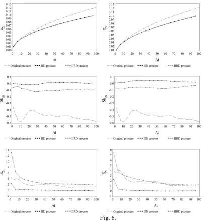
Fig. 6 displays a symmetric RRG. We get L₁ =L₂ from maximum likelihood

estimates. Kurtosis behavior in the IIDR process is very similar to actual value. This suggests that kurtosis behavior can be explained in terms of the time evolution characterizing the RRG. Skewness behavior is not that clear-cut, however. This is

somewhat expected because the generator is symmetric, and A = 0. Standard deviation

behaves as if the process had a Hurst exponent of ½.

8 Concluding remarks

This paper approaches the issue of the sum of stochastic variables and take independent processes that are identically distributed in their reduced variables as well as autocorrelated processes that are identically distributed. We extend the classic central limit theorem that features finite variance.

The paper also examines cases where a formation law for series’ variance is present. Our suggested reduced variable (that is independent and identically distributed) seems to fit

well a financial data set sampled from the intraday Brazilian real-US dollar rate of year

2002. We find the reduced variable together with an exponential law to mimic the series’ volatility behavior. And we also find the reduced variable to fail reaching zero as sample size approaches infinity.

We too investigate the role of nonlinear autocorrelations in the dynamics of convergence to a Gaussian. We find sluggish convergence to be due to the nonlinear autocorrelations.

Thus some features of the nonlinear autocorrelations can be rationalized in terms of an independently distributed, reduced process. Information about the autocorrelations is already encompassed in mean and standard deviation’s time paths. This is in line with the fact that a process is independent but not identically distributed. Nonidentity satisfactorily explains slow convergence to the Gaussian regime as well as greater-than-½ Hurst exponents. And it is possible to observe a non-IID behavior of skewness and kurtosis even when the Hurst equals ½.

Nonconvergence to a Gaussian is thus explained by departures from the infinitesimality hypothesis of independently distributed, reduced processes.

Acknowledgements

References

Bavly, G. M. (1936) Über einige Verallgemeinerungen der grenzwertsätze der Wahrsheinlichkeitrenchnung, Sbornik., 1, 917-930.

Feller, W. (1935) Über den Zentralen Grenzwertsatz der Wahrsheinlichkeitrenchnung,

Math. Zeitshirift, 40, 521-529.

Feller, W. (1937) Über den Zentralen Grenzwertsatz der Wahrsheinlichkeitrenchnung,

Math. Zeitshirift, 42, 301-312.

Feuerverger, A. and Mureika, R. (1977) The empirical characteristic function and its applications, The Ann. of Statist., 5, 88-97.

Feuerverger, A. and McDunnough, P. (1981) On the efficiency of empirical characteristic function procedures, J. R. Statist. Soc. B, 43 (1), 20-27.

Figueiredo, A., Gleria, I., Matsushita and R., Da Silva, S. (2003) On the origins of truncated Levy flights, Phys. Lett. A, 326, 51-60.

Figueiredo, A., Gleria, I., Matsushita, R. and Da Silva, S. (2004) Levy flights,

autocorrelation, and slow convergence, Physica A, 337, 369-383.

Figueiredo, A., Gleria, I., Matsushita, R. and Da Silva, S. (2005) Financial volatility and independent and identical distributed variables, Physica A, 346 (2005), 484-498.

Finetti, B. (1929) Sulla funzione a incremento aleatorio, Tai. Acad. Naz. Lincei., 6,

163-168, 325-329, 548-553.

Gnedenko, B. V. and Kolmogorov, A. N. (1954) Limit distributions for sums of

independent random variables, Reading: Addison-Wesley.

Khintchine, A. J. (1938) Limit laws for sums of independent random variables, Moscow:

ONTI.

Kolmogorov, A. N. (1921) Über die summen durch Zuffal bestimmter unabhängiger Gröβen, Mathematishe Annalen,99, 309-319.

Levy, P. (1922) Sur la loi de Gauss, C. R. Acad. Sc., 174, 1682-1684.

Levy, P. (1924) Théorie des erreurs. La loi de Gauss et les lois exceptionelles, Bull. Soc.

Math. France, LII, 49-85.

Levy, P. (1929) Sur quelques travaux relatifs à la théorie de errers, Bull. Soc. Math. France,

Liapunoff, A. M. (1900) Sur une proposition de la théorie dês probabilités, Bull. De L´Acad. Des Sciences St. Petersbourg, 13, 359-386.

Lindberg, J. W. (1922) Eine neue herleitung des Exponentialgesetzes in der

Wahrsheinlichkeitrenchnung, Math. Zeitschrift, 15, 211-225.

Mantegna, R. N. and Stanley, H. E. (1994) Stochastic process with ultraslow convergence to a Gaussian, the truncated Levy flight, Phys. Rev. Lett., 73, 2946-2949.

Mantegna, R. N. and Stanley, H. E. (1995) Scaling behavior in the dynamics of an economic index, Nature, 376, 46-49.

Zolotarev, V. M. (1990) Reflections on the classical theory of limit theorems, Theory

Probab. Appl., 36 (1), 124-137.

Zolotarev, V. M. (1965) On the closeness of distributions of two sums of independent

random variables, Theory Probab. Appl., 10 (1965), 519-526.

Zolotarev, V. M. (1997) Modern theory of summation of random variables, Modern

Probability and Statistics, Utrecht: VSP.

Estimated Value ± Standard Error IIDR

Exponential lawm_i = Ae−Bi

A = 0.0156 ± 0.000599

B = 0.2070 ± 0.0101

IIDR

Power law B

i Ai

m = −

A = 0.0149 ± 0.000899

B = 0.7711 ± 0.0521

IIDR

Power law m_i =(A+iB)−1/C

[image:27.612.81.432.85.233.2]

A = 4.2267 ± 1.3063 B = 0.4973 ± 0.3191 C = 0.3607 ± 0.0807 Table 1. Estimated models

Experimental Data IID IIRD Exponential Law Power Law Power Law

Skewness 1.5287 0.6854 1.3497 1.3086 1.4296 1.3493

Kurtosis 19.3846 5.7230 25.6804 23.9674 31.0246 25.5359

Table 2. Skewness and kurtosis of experimental data under alternative assumptions

[image:27.612.78.533.288.333.2]

[image:28.612.208.406.70.214.2] [image:28.612.210.407.273.412.2]

Fig. 1. Brazilian real-US dollar 15-minute spaced returns for year 2002

Fig. 2. Standard deviations m_i against i

Fig. 3. Fitting exponential law Bi

i Ae

[image:28.612.210.408.454.593.2]

[image:29.612.93.496.70.230.2]

(a) (b)

Fig. 4. Behavior of kurtosis (a) and skewness (b) for daily returns of the pound-dollar rate Curves for an IID process are shown for comparison

(a) (b)

Fig. 5.

[image:29.612.87.494.286.471.2]

[image:30.612.91.495.80.521.2]

Fig. 6.

Scaling in standard deviations (upper panel), skewness (mid panel) and kurtosis (lower panel) of daily observations of the pound-dollar rate

The IIRD process on left plots is generated with P = 5, A = 0, and symmetric case L = L1 =

L2

The maximum likelihood estimate of L is 7.52