Discriminant Neighborhood Structure Embedding Using Trace Ratio Criterion for Image Recognition

http://dx.doi.org/10.4236/jcc.2015.311011

Discriminant Neighborhood Structure

Embedding Using Trace Ratio Criterion for

Image Recognition

Jing Wang1, Fang Chen1, Quanxue Gao1,2

1_{School of Telecommunications Engineering, Xidian University, Xi’an, China}

2_{State Key Laboratory of Integrated Services Networks, Xidian University, Xi’an, China}

Received September 2015

Abstract

Dimensionality reduction is very important in pattern recognition, machine learning, and image recognition. In this paper, we propose a novel linear dimensionality reduction technique using trace ratio criterion, namely Discriminant Neighbourhood Structure Embedding Using Trace Ratio Criterion (TR-DNSE). TR-DNSE preserves the local intrinsic geometric structure, characterizing properties of similarity and diversity within each class, and enforces the separability between ferent classes by maximizing the sum of the weighted distances between nearby points from dif-ferent classes. Experiments on four image databases show the effectiveness of the proposed ap-proach.

Keywords

Dimensionality Reduction, Manifold Learning, Variability, Trace Ratio

1. Introduction

Linear discriminant analysis (LDA) has been used widely in pattern recognition, machine learning, and image recognition [1] [2]. However, methods based on LDA techniques are optimal under Gaussian assumption [3] [4] and they effectively capture only the global Euclidean structure which may impair the local geometrical struc-ture of data [5]-[7]. Recently, many approaches have shown the importance of local geometrical strucstruc-ture for dimensionality reduction and image classification. One of the most popular linear approaches is neighbourhoods preserving embedding (NPE) [8]. NPE aims to discover the local structure of the data and find projection direc-tions along which the local geometric reconstruction reladirec-tionship of data can be preserved.

Motivated by NPE, many discriminant approaches have been developed to further improve the data classifi-cation accuracy [9]-[11], such as margin fisher analysis (MFA) [12], locality sensitive discriminant analysis (LSDA) [13], locally linear discriminant embedding (LLDE) [14] and discriminative locality alignment (DLA) [15]. They preserve the intrinsic geometrical structure by minimizing a quadratic function.

data representation and classification [13] [16]-[19]. By maximizing the variance, we can unfold the manifold structure of data and may preserve the geometry of data. Structure of real-world data is complex and unknown, thus a single characterization may not be sufficient to represent the underlying intrinsic structure. It indicates that none of the aforementioned approaches can detect a stable and robust intrinsic structure representation.

In this paper, we propose a novel dimensionality reduction approach, namely discriminant neighbourhood structure embedding using trace ratio criterion (TR-DNSE) which explicitly considers the global variation, local variation, and local geometry. Experiments on four image databases indicate the effectiveness of TR-DNSE.

The remainder of this paper is organized as follows: Section 2 analyzes NPE. The idea of TR-DNSE is pre-sented in Section 3. Section 4 describes some experimental results. Section 5 offers our conclusions.

2. Problem Statements

Given training data matrix X =

[

x x_{1 2}x_N

]

, where xi∈Rn

(

i=1,,N

)

denotes the i-th training data, N is

the number of training data. The objective function of NPE is [8]

*

arg min

T T

T T

XMX XX

α α

α

α α

= (1)

where α denotes a projection matrix, M =

(

IN −W

) (

T IN−W

)

. The elements Wij in weight matrix W

denote the coefficients for reconstructing xi from its neighbours

{ }

xj , and can be calculated using [6].

The objective Function (1) can be decomposed into the following two objective functions:

minαT_XMXTα

(2)

maxαTXXTα (3)

The objective Function (2) aims to preserve the intrinsic geometry of the local neighborhoods [6] [8]. Given that all data points are centered, i.e. x=1 N

∑

_ix_i =0, then the objective function (3) becomes

(

)(

)

, 1

1 max

2

N _T

T

i j i j

i j

x x x x

Nα = α

 

− −

 



∑

 (4)

Obviously, the objective function (4) which is equal to principal component analysis [2] aims to preserve the amount of variation of the values of data in the reduced space. However, it results in the following problems. It distorts the local geometry of data. As aforementioned analysis, the objective function (4) does not detect the local discriminating information among the nearby data points. Furthermore, NPE is an unsupervised approach, which does not make good use of the label information. It means that the generalization ability and stableness of NPE are not good enough.

3. Discriminant Neighborhood Structure Embedding Using Trace Ratio Criterion

3.1. The Objective Function for Dimensionality Reduction

Given training data matrix X =

[

x x1 2xN

]

, where

n i

x ∈R

(

i=1,,N

)

denotes the i-th training data, N is the number of training data. τi denotes the class label of data xi. Motivated by manifold learning approaches

[6] [8] [18]-[20], we construct two adjacency graphs, namely geometry graph Gg=

{ }

Z S, and variability graph G_v=

{ }

Z B, , with a vertex set Z =

{

x i_i, =1,,N

}

and two weight matrices S and B, to model the local geometry and variation of data, respectively. The elements S_ij can be calculated by the following [6] [8]:

2

min _{i j ij j}

i

x S x

 ₋ 

 



∑

∑

 (5)

From the viewpoint of statistics, if two points xi and xj are very close to each other,

2

i j

x −x ( •

de-notes the Euclidean distance between two vectors) is small, then the amount of variation of the values between them is also small. According to the analysis, the elements Bij can be defined as follows:

(

2

)

exp , ( ) , ( )

0 , Otherwise

i j i k j j k i i j

ij

t x x if N N and

B

 _{− − ∈ ∈ =}

 =  

x x x x τ τ

(6)

where N_k(x_i) is k nearest neighbors of xi, t≥0 is a positive parameter.

Moreover, motivated by LDA [1], we construct two global graphs Gw=

{

Z M, w

}

and Gb=

{

Z M, b

}

over

the training data points to model the global variation, where, Mw

( )

i j, =1 /nc and Mb

( )

i j, =1 /N−1 /nc if

i j

τ =τ , and M_w

( )

i j, =0 and M_b

( )

i j, =1 /N. nc is the number of the samples in the c-th class. The cor-

responding Laplacian matrices are denoted as Lw and Lb and L= −D S, where D is a diagonal matrix

with the D i i

( )

, =

∑

_jS i j

( )

, . As shown in [20], the between-class scatter matrix Sb and the within-class

scatter matrix Sw can be rewritten as

T

w w

S =XL X and Sb =XL Xb T.

The goal of TR-DNSE is to find projection directions such that both the amount of variation of values of data and local geometry can be preserved in the reduced space. A reasonable criterion for choosing a good map is to optimize the following four objective functions

2

min _{i ij j}

j i

y S y

 ₋ 

 



∑

∑

 (7)

(

)

2

max _{ij i j}

ij

B y y

 

−

 



∑

 (8)

(

)

maxtr YL Yb T (9)

(

)

mintr YL Yw T (10)

where yi denotes the low-dimensional representation of xi, Y =

(

y y1, 2,,yN

)

.

The objective function (7) ensures that the weights, which reconstruct the point xi by its same class datasets

in the high dimensional space, will well reconstruct yi by the corresponding datasets points in the low

dimen-sional space. The objective function (10) ensures the data points from the same class will be closer than data from different class. The objective function (9) emphasizes the large distance data pairs. Maximizing (8) is an attempt to ensure that, if the amount of variation of the values between xi and xj is large, then the amount of

variation between yi and yj is also large. By simultaneously solving the four objective functions, we can

obtain reasonable projection directions such that the variation and geometry of data can be well detected in low- dimensional space.

3.2. Optimal Linear Mapping

Suppose α is a projection matrix, that is, yi=αTxi. By simple algebra formulation, the objective function (7)

and (8) can be reduced to

2

T T

i j ij j i

y − S y =α X M X α

∑

∑

(11)

(

)

2

(

)

2 T T

ij i j d

ij

B y −y = α X L X α

∑

(12)

where IN is a N-dimensional identity matrix,

(

) (

)

T

N N

M = I −S I −S , Ld=H−B, B is a N×N

ii j ji j ij

F =

∑

B or

∑

B . Finally, the optimization problem in ratio trace criterion can be reduces to finding:

(

)

* arg max T T b T T d w XL X

X M L L X

α α α α α     =   − +  

  (13)

3.3. Discriminant Neighborhood Structure Embedding Using Trace Ratio Criterion

Generally, the objected function (13) can be solved by using generalized eigenvalue decomposition. Given that the low-dimensional data representation is F. F is constrained to be in the linear subspace spanned by the training data matrix X. As shown in [21], we relax the hard constraint by substituting XTα by F and

add-ing a regression residual term _F−_XTα 2 _{into the reformulated objective function. Then, F is enforced to}

be close to T

X α. Specifically, we propose the following objective function:

(

)

(

)

(

)

2

( )

,

*, * argmax

T

T b

T T T

F I

a

Tr F L F F

Tr F L F X F Tr

α α

α

α β α α

=

=

+ − + (14)

(

)

(

_T

)

(

(

_T

)

_T 2

(

_T

)

)

t Tr F L Ft b t Tr F L Ft a t X t Ft Tr t t

λ = + α − +β α α (15)

where β is a parameter to balance different terms and La=M −Ld+Lw.

The above optimization problem in (14) is solved by Algorithm 1.

Explanation of Algorithm 1: With λt from the t-th iteration in (16), Ft+1 and αt+1 are computed by

max-imizing the following trace different problem:

(

1 1

)

(

(

)

)

(

)

(

)

( )

,

, argmax 2

T

T T T T T

t t b t a t t t t

F I

F Tr F L L I F Tr XF Tr XX Tr

α α

α λ λ λ α λ α α λ β α α

+ +

=

= − − + − − (16)

From (16), it can be observed that

(

,

)

t

U_λ F α is a concave quadratic function with respect to the variable F

when the matrix

(

Lb−λtLa−λtI

)

is negative-definite. We set the partial derivative of Uλ_t

(

F,α

)

with

re-spect to the variable F as zero, namely

(

,

)

₍

₍

₎

₎

2 0

t T T

b t a t t t

U F

L F L F F X F V X

F

λ α _{λ λ α λ α}

∂

= − − − = ⇒ =

∂ (17)

where Vt

(

λtI λtLa Lb

)

1

−

= + − . In most cases, the matrix

(

λtI λtLa Lb

)

1

−

+ − is negative-definite in our

experi-ments, and

(

λtI λtLa Lb

)

1

−

+ − is symmetric. Substituting F in (16) by (17), then we get:

(

)

(

)

(

)

(

2 1

)

1 argmax

T

T T

t t t t a b t

I

Tr X I L L I X

α α

α α λ λ λ − λ α

+

=

= + − − (18)

Algorithm 1. TR-DNSE algorithm.

Input: t=1, α=Iˆ, ˆ f d

I∈R× Iˆii=1, for i=(1,,d), and 0 otherwise. While 4

1 ( 10 )

t t

λ λ ξ ξ −

+ − 〈 = :

Compute λt by Equation(15);

Update αt+1 as the eigenvectors corresponding to the d largest eigenvalues of the matrix

(

( )

)

1

2 T

t t t a b t

X λ λI+λL −L − −λI X ;.

Update 1 ( )1 1

T

t t t t a b t

F+ =λ λI+λL −L − X α+ ;.

1

t= +t ;

In (18) we use the property Lb-λtLa λtI V- t 1

−

= . We also have

( )

T

Tr α α =d because T

I

α α= . Hence,

1 t

α+ is composed of the eigenvectors corresponding to the d largest eigenvalues of the matrix

(

)

(

2 1

)

T

t t t a b t

X λ λI+λL −L − −λI X , which explains the step 3 in Algorithm 1.

4. Experiments

In this section, we employ four widely used image databases (YALE, PIE, FERET and COLL20) to evaluate the performance of TR-DNSE and compare it with some classical approaches including Fisher face [22], MFA [12], LSDA [13], DLA [14] and LLDE [15] in the experiments. In classification stage, we use the Euclidean metric to measure the dissimilarity between two feature vectors and the nearest classifier for classification.

In our experiments, we first use the PCA to reduce the dimension of the training data by keep 80% - 97% energy of images. Likewise, we empirically determine a proper parameter k within the interval

[

1,N−1

]

and parameter t within the interval

(

0,∞

)

for the corresponding approaches.

The CMU PIE database [23] contains 68 subjects with 41368 face images as a whole. We select pose-29 im-ages as gallery that includes 24 samples per person. The training set is composed of the first 12 imim-ages per per-son, and the corresponding remaining images for testing. Moreover, each image is of the size 64 64× .

The Yale Face Database contains 165 grayscale images of 15 individuals. There are 11 images per subject. In our experiments the images are normalized to the size of 32 32× . The first six images are selected to be the training data, and the rest for testing.

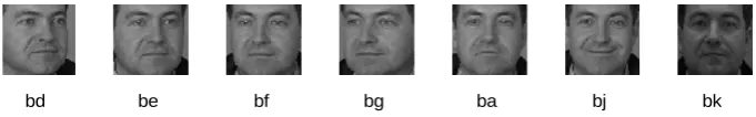
The FERET database [24] includes 1400 images of 200 individuals (each with seven images). All the images were cropped and resized to 80 80× pixels. The images of one person are shown in Figure 1. In the experi-ment, we choose four images per person for training, and the remaining images from for testing.

The COIL20 image library contains 1440 gray scale images of 20 objects (72 images per object) [25]. Each image is of size 32 32× . In the experiments, we select the first 36 images per object for training and the re-maining images for testing.

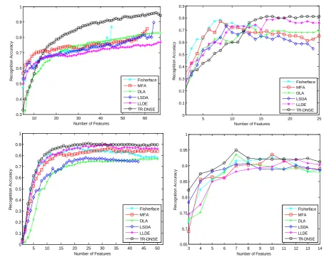
Table 1 shows the best results of six approaches on four databases. Figure 2 plot the curves of recognition accuracy vs. number of projected vectors on four databases.

[image:5.595.142.483.485.538.2]

TR-DNSE has the best recognition accuracy than the other approaches in all the experiments. This is probably due to the fact that TR-DNSE preserves both the local geometry and variation of data, especially the discrimi-nating information embedded in nearby data from different classes. Different from other approaches, TR-DNSE approach has a trace ratio criterion in solution. Related work demonstrates that the projection matrix solved

[image:5.595.88.540.579.718.2]

Figure 1. Some sample images of one subject in the FERET database.

Table 1. Top recognition accuracy (%) of six approaches on four databases and the corresponding number of features.

Database PIE YALE FERET COIL20

Methods Recognition Dimension Recognition Dimension Recognition Dimension Recognition Dimension

Fisherface 86.89 45 77.33 8 87.17 21 92.64 10

MFA 85.66 61 73.33 8 86.5 32 93.61 10

LSDA 89.58 64 73.33 9 78 27 92.78 21

DLA 89.58 189 73.33 13 76.83 38 93.61 7

LLDE 93.63 101 80 18 89.83 31 92.08 12

TR-DNSE 95.96 65 81.33 16 90.83 39 95 7

[image:6.595.81.536.81.442.2]

Figure 2. Recognition accuracy vs. number of projection vectors on the four databases.

by using trace ratio criterion is generally better than the projection matrix solved by using generalized eigenva-lue decomposition. By the trace ratio criterion, we can get an orthogonality projection matrix which helps to un-fold the geometry and encode discriminating information of data. So the trace ratio criterion of TR-DNSE helps to get a better projection which results in better results.

5. Conclusion

Our method, TR-DNSE, which is proposed for dimensionality reduction, incorporates the intrinsic geometry, local variation, and global variation into the object function of dimensionality reduction. Geometry guarantees that nearby points can be mapped to a subspace in which they are still very close, which characterizes the simi-larity of data. Global variation and local variation characterize the most important modes of variability of pat-terns, and help to unfold the manifold structure of data and encode the discriminating information, especially the discriminating information embedded in nearby data from different classes. Experiments on four real-world im-age databases indicate the effectiveness of our TR-DNSE approach.

References

[1] Fukunaga, K. (1990) Introduction to Statistical Pattern Recognition. 2nd Edition, Academic Press.

[2] Jolliffe, T. (1986) Principal Component Analysis. Springer-Verlag, New York.

http://dx.doi.org/10.1007/978-1-4757-1904-8

[3] Strassen, V. (1969) Gaussian Elimination Is Not Optimal. Numer Math., 13, 54-356.

http://dx.doi.org/10.1007/BF02165411

10 20 30 40 50 60 0.3 0.4 0.5 0.6 0.7 0.8 0.9 1

Number of Features

R ec ogni ti on A c c ur ac y Fisherface MFA DLA LSDA LLDE TR-DNSE

5 10 15 20 25

0 0.1 0.2 0.3 0.4 0.5 0.6 0.7 0.8 0.9

Number of Features

R ec ogni ti on A c c ur ac y Fisherface MFA DLA LSDA LLDE TR-DNSE

5 10 15 20 25 30 35 40 45 50 0 0.1 0.2 0.3 0.4 0.5 0.6 0.7 0.8 0.9 1

Number of Features

R ec ogni ti on A c c ur ac y Fisherface MFA DLA LSDA LLDE TR-DNSE

3 4 5 6 7 8 9 10 11 12 13 14 0.65 0.7 0.75 0.8 0.85 0.9 0.95 1

Number of Features

[4] Tao, D., Li, X., Wu, X. and Maybank, S.J. (2007) General Tensor Discriminant Analysis and Gabor Features for Gait Recognition. IEEE Trans. Pattern Anal. Mach. Intell., 29, 1700-1714. http://dx.doi.org/10.1109/TPAMI.2007.1096

[5] Saul, L.K. and Roweis, S.T. (2003) Think Globally, Fit Locally: Unsupervised Learning of Low Dimensional Mani-folds. J. Mach. Learn. Res., 4, 119-155.

[6] Roweis, S. and Saul, L. (2000) Nonlinear Dimensionality Reduction by Locally Linear Embedding. Science, 290, 2323-2326. http://dx.doi.org/10.1126/science.290.5500.2323

[7] Belkin, M. and Niyogi, P. (2003) Laplacian Eigenmaps for Dimensionality Reduction and Data Representation. Neural Computation, 15, 1373-1396. http://dx.doi.org/10.1162/089976603321780317

[8] He, X., Cai, D., Yan, S. and Zhang, H. (2005) Neighbourhood Preserving Embedding. Proc. ICCV.

[9] Lai, Z., Wan, M., Jin, Z. and Yang, J. (2011) Sparse Two-Dimensional Local Discriminant Projections for Feature Ex-traction. Neurocomputing, 74, 629-637. http://dx.doi.org/10.1016/j.neucom.2010.09.010

[10] Yu, J., Liu, D., Tao, D. and Seah, H.S. (2011) Complex Object Corresponding Construction in Two-Dimensional Animation. IEEE Trans. Image Processing, 20, 3257-3269. http://dx.doi.org/10.1109/TIP.2011.2158225

[11] Xu, Y., Feng, G. and Zhao, Y. (2009) One Improvement to Two-Dimensional Locality Preserving Projection Method for Use with Face Recognition. Neurocomputing, 73, 245-249. http://dx.doi.org/10.1016/j.neucom.2009.09.010

[12] Xu, D., Yan, S., Tao, D., et al. (2007) Marginal Fisher Analysis and Its Variants for Human Gait Recognition and Content-Based Image Retrieval. IEEE Transactions on Image Processing, 16, 2811-2821.

http://dx.doi.org/10.1109/TIP.2007.906769

[13] Gao, Q., Xu, H., Li, Y. and Xie, D. (2010) Two-Dimensional Supervised Local Similarity and Diversity Projection, Pattern Recognition, 43, 3359-3363. http://dx.doi.org/10.1016/j.patcog.2010.05.017

[14] Zhang, T., Tao, D., Li, X. and Yang, J. (2009) Patch Alignment for Dimensionality Reduction. IEEE Trans. Knowl. Data Eng., 21, 1299-1313. http://dx.doi.org/10.1109/TKDE.2008.212

[15] Li, B., Zheng, C.H. and Huang, D.S. (2008) Locally Linear Discriminant Embedding: An Efficient Method for Face Recognition. Pattern Recognition, 41, 3813-3821. http://dx.doi.org/10.1016/j.patcog.2008.05.027

[16] Weinberger, K.Q. and Saul, L.K. (2004) Unsupervised Learning of Image Manifolds by Semi-Definite Programming. Proc. IEEE Con. Computer Vision and Pattern Recognition’2004, 988-995.

http://dx.doi.org/10.1109/CVPR.2004.1315272

[17] Weinberger, K.Q., Packer, B.D. and Saul, L.K. (2005) Nonlinear Dimensionality Reduction by Semi-Definite Pro-gramming and Kernel Matrix Factorization. Proc. the Tenth Workshop Artificial Intelligence and Statistics (AISTATS- 2005), 381-388.

[18] Zhou, T., Tao, D. and Wu, X. (2011) Manifold Elastic Net: A Unified Framework for Sparse Dimension Reduction. Data Min. Knowl. Disc., 22, 340-371. http://dx.doi.org/10.1007/s10618-010-0182-x

[19] Gao, Q., Zhang, H. and Liu, J. (2012) Two-Dimensional Margin, Similarity and Variation Embedding. Neurocomput-ing, 86, 179-183. http://dx.doi.org/10.1016/j.neucom.2012.01.023

[20] Yan, S., Xu, D., Zhang, B., Zhang, H., Yang, Q. and Lin, S. (2007) Graph Embedding and Extensions: A General Framework for Dimensionality Reduction. IEEE Trans. Pattern Anal. Mach. Intell., 29, 40-51.

http://dx.doi.org/10.1109/TPAMI.2007.250598

[21] Nie, F., Xiang, S. and Zhang, C. (2007) Neighbourhood Minmax Projections. IJCAI-07, 993-998.

[22] Belhumeur, P., Hespanha, P. and Kriegman, D. (1997) Eigenfaces vs. fisherfaces: Recognition Using Class Specific Linear Projection. IEE Trans. Pattern Anal. Mach. Intell., 19, 711-720. http://dx.doi.org/10.1109/34.598228

[23] Gao, Q., Liu, J., Zhang, H., Hou, J. and Yang, X. (2012) Enhanced Fisher Discriminant Criterion for Image Recogni-tion. Pattern Recognition, 45, 3717-3724. http://dx.doi.org/10.1016/j.patcog.2012.03.024

[24] Phillips, P., Moon, H., Rizvi, S. and Rauss, P. (2000) The FERET Evaluation Methodology for Face-Recognition Al-gorithms. IEEE Trans. Pattern Anal. Mach. Intell., 22, 1090-1104. http://dx.doi.org/10.1109/34.879790