Load Balancing Approach for Scheduling Sequential
Task in Grid Computing Environment
Neeraj Pandey
Department of Computer Science & Engineering G. B. Pant Engineering College
Ghurdauri, UK, India
Shashi Kant Verma
Department of Computer Science & Engineering G. B. Pant Engineering College
Ghurdauri, UK, India
Vivek Kumar Tamta
Department of Computer Science & Engineering G. B. Pant Engineering College
Ghurdauri, UK, India
ABSTRACT
In grid computing environment, the efficiency of computing node is affected by several factors such as node utilization, allocation of jobs etc. The incoming job is allocated to appropriate node in such a way that the node utilization is maximized and a well-balanced load across all the participating computing nodes that enhances the overall performance of grid computing. This paper presents an amended hybrid approach for scheduling sequential task. The proposed approach uses combination of first-come-first-served (FCFS) and genetic algorithm (GA). A sliding-window technique is presented to initiate alteration between the FCFS and GA, to offers a rapid task assignment. For GA we initially generate random population and use straightforward encoding. The proposed method is evaluated in the terms of makespan value and node utilization with a varying set of simulation cases and parameters after then it is compared with a well design first-come-first-server (FCFS) and hybrid genetic algorithm (HGA). Experimental results have shown significant improvement compared to the both FCFS and HGA algorithms. The result gives minimized makespan value with increased node utilization for both homogeneous and heterogeneous types of nodes.
Keywords
Grid Computing, Load Balancing, Task Scheduling, Genetic Algorithm, Performance evaluation
1.
INTRODUCTION
A grid computing environment consist aggregations of both homogeneous and heterogeneous resources and provide infrastructure for solving problems for any stand-alone machine. The main focus of grid computing is large-scale resource sharing, innovative application and, in some case high-performance orientation [1]. There are various computing application that requires high performance computing resources to process the job and lead to increase overall execution time for job and thus decreases the node utilization and overall system performance. A “task” is a small segment of program and it has equal probability to scheduled individually in any of the computing node. A computing node within a grid environment is a processor that receive tasks from a centralized queue. Different nodes have different task/job processing capabilities, different memory segment and because of heterogeneous nature of computing node a load imbalance exists between nodes therefore a special load balancing scheme is needed to manage this load imbalance effectively. The scheduling of jobs is primarily concerned for the proper functionality of a grid computing system.
Genetic algorithms [3,4,8,9,10,13,14,16] are search heuristics, to find optimal solution job scheduling as compared to other search procedures. It is a method for solving optimization problems and based on process of natural genetics.
The First-Come-First-Serve (FCFS) algorithm [4,5,10] is a simple job scheduling algorithm in which task executed according to their arrival pattern in the job queue and the job which arrived earlier will be executed first. Consider a grid environment consists of m computing nodes Ni given as:
Ni = {N1, N2, N3, ……,Nm} . (1)
Where each computing nodes has its own capability Ci to
execute the task and given as:
Ci = {C1, C2, C3, ……,Cm} . (2)
Since each task require some memory segments (Ms),
processing power (Pp), and input/output (Io) function,
therefore the capacity of a node can be defined as a three tuple element given as:
C = {Ms, Pp, Io} . (3)
A group of n task Tj which is executed on Pi is given as:
Tj = {T1, T2, T3, ………, Tn} . (4)
Since every task has a start time Ts, an end time Te, an arrival
time Ta, and a computational duration Tx, therefore we can
define a task as a group of 4 elements and given as:
{Ts, Te, Ta, Tx) = {Tsj, Tej, Taj, Txj} . (5)
A task can be scheduled to any of the node involve in grid system, so the execution time of the task is determined by the dividing the computational time of the task to the capacity of the computing node.
Texe = Tx / c . (6)
The final goal of FCFS is minimize the execution time of the task. i.e.,
Texe = min {Texe | ∀ Ni} . (7)
This paper present an amended hybrid job scheduling approach [4] based on FCFS and genetic algorithm in distributed computing environment. We also design the FCFS and HGA approach for job scheduling and compare the proposed algorithm to these algorithm. The proposed algorithm contain traditional scheduling heuristics to generate a feasible solution by determining the status of computing node and their capability to execute the task.
2.
RELETED WORK
K. Q. Yan et al. [10] proposed a hybrid load balancing policy which integrated static and dynamic load balancing technologies to assist in the selection for effective nodes. Essentially, a static load balancing policy is applied to select effective and suitable node sets. The task first divided into independent subtasks and after then minimum resource demand is taken. The execution of task are done according to value estimated by a value function.
A task allocation algorithm based on multi-heuristic evolutionary approach for heterogeneous distributed system is presented in [16]. It manoeuvres on batches of unmapped tasks and tasks are dynamic and pre-emptive in nature. It operates dynamically, and allow each tasks for continuous execution. The main involvement is on-line estimation of resources where resources are varying in nature, dynamic model for task execution and the scheduling method with no prior knowledge.
In the last few year genetic algorithm becomes very popular to solve load balancing problem. There are numerous studies on scheduling method for computational grid environment. Zomaya and Hwei [3] present a centralized methods for load balancing based on genetic algorithm. The number of tasks are fixed and allocation of task to the node is done when a predefine criteria is met. Also they suppose that there are always adequate task in the waiting queue ready to process and the characteristics of task is known earlier before scheduling it.
Yajun Li et al. [4] address the load balancing problem by presenting a hybrid approach to the load balancing of sequential tasks under grid computing environments. Two policy that are used for scheduling is FCFS and genetic algorithm and tasks are scheduled according to policy used. In centralized queue, when number of task becomes equal to sliding window size the genetic algorithm start its functioning. The results are compared with the FCFS and dynamic GA with improvement in terms of makespan, mean deviation and node utilization.
Junwei Cao et al. [5] demonstrates that AI techniques can be utilized to achieve effective workload and resource management. A combination of intelligent agents and multi-agent approaches is applied to both local grid resource scheduling and global grid load balancing. The grid agents are controlled by a centralized mechanism and each agent have previous knowledge of all other agents.
Zomaya et al. [8] present a genetic algorithm based solution for the problem of task scheduling. There is no need to apply any problem specific assumptions such is the case when using heuristics. The tasks are dependent in nature i.e., precedence constraints exists between tasks and a priority is assigned to each task before they added to a list of waiting tasks.
A grid system can be affected by various factors such as system failures, node availability, and communication delay. Shanshan Song et al. [9] models the risk and insecure conditions in Grid job scheduling and propose six risk-resilient scheduling algorithms to assure secure Grid job execution under different risky conditions. The encoding methods for GA is based on the messy encoding concept and the initial population is based on the prior solution. A job failure model is also developed including three risk springy methods such as pre-emptive, delay tolerant, and replication for scheduling of grid jobs.
3.
SYSTEM MODEL
In this Section, we first present the system model, followed by the OMNeT++ simulation model.
3.1
System Model
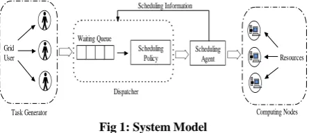
The system model assumed in this paper consists of n computing nodes where each node has its own capacity Ci. Nodes are connected to each other through a communication channel. we also assume that there exist a centralized scheduling scheme, in which all the task arrive at a central queue, at the scheduler. The tasks coming from the grid users are first placed in a task queue and the task scheduler schedule the task according to the policy used such as FCFS or genetic algorithm. The scheduler makes sure that queue is filled with a minimum number of tasks for execution (in case of genetic algorithm).
A near-optimal schedule based on genetic algorithm is determined by the scheduler. The task scheduler schedule the job to appropriate node. The scheduling model is given in fig.1. The scheduling algorithm has full knowledge about the available computing node or resources and current workload, when making decision to schedule the current task. A scheduling agent is able to estimate all statistics information and responsible to provide all necessary information to task dispatcher to make the scheduling decision. Because of limited availability of network resources (nodes), nodes does not contain a waiting queue for tasks.
Grid User
Waiting Queue
Scheduling Policy
Scheduling
Agent Resources
Task Generator Computing Nodes
Dispatcher
[image:2.595.318.541.368.464.2]Scheduling Information
Fig 1: System Model
The waiting queue consists of a large number of unscheduled tasks. If all of tasks available in waiting queue scheduled at once, it take a long time to proceed as well as find an efficient schedule, thus it increase the overall processing time of the system and give the chance to the computing node to become in ideal state. To minimize and eliminate this condition we only consider a small subset of these waiting tasks, hence a sliding window mechanism is used.
3.2
OMNeT++ Model
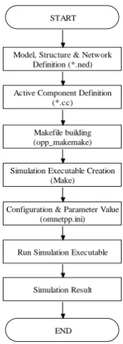
OMNeT++ (Objective Modular Network Testbed in C++) [6,7] is an public source, component based, modular and open-architecture event discrete simulation environment used by various research groups for communication network performance evaluation. Because of its generic and flexible architecture, it has been successfully used in other areas like the simulation of IT systems, queuing networks, hardware architectures and business processes as well [15]. An OMNeT++ model consists of the following parts:
Message definitions files (with .msg suffix) represent job or task to be scheduled.
Network Description files (with .ned suffix) shows the components of the simulated network in a graphical manner.
Simple modules implementation (with .cc suffix).
Model, Structure & Network Definition (*.ned)
Active Component Definition (*.cc)
Makefile building (opp_makemake)
Simulation Executable Creation (Make)
Configuration & Parameter Value (omnetpp.ini)
Run Simulation Executable
Simulation Result START
END
Fig 2: Flow Chart for Simulation using OMNeT++
The flow chart for OMNeT++ simulation for our proposed algorithm is given in fig. 2. There are 4 modules of simulation model given as:
Task generator
Grid agent
Dispatcher
Computing node
The Task generator produces the task and these tasks are stored in a centralized task queue. The task generated by task generator are mutually independent i.e., there is no precedence constraint exists between the task.
If tasks are arriving in the queue at the exponentially distributed rate λ, then the probability that there will be n tasks after time t is given as:
! nt n
t
P t e
n
(8)
The inter-arrival time, , is the average time between task arrivals, measured in time per task and given as:
= 1 / λ . (9)
The dispatcher schedule the task to an appropriate node. To make enhanced scheduling decision, grid agent collects all the pertinent information such as node capacity and provide it to the dispatcher. The dispatcher module consist all 3 algorithm: first-come-first-served (FCFS), hybrid genetic algorithm (HGA), and proposed amended hybrid genetic algorithm (AHGA). The task get schedule to appropriate node according to the policy used. More precisely, proposed approach for task scheduling is to divide-the scheduling function into 2 phase. In first phase the task get scheduled according to the FCFS policy. The second phase start when the number of task in sliding window reaches its size and it start the GA. Again we emphasize that the grid agent has adequate knowledge about the characteristics of task placed in waiting queue, available nodes and system that help to make an impeccable scheduling decision. The process of scheduling in grid can be categorized in two parts: static or deterministic and dynamic or stochastic.
This paper presents a deterministic scheduling approach in which, the arrival times of tasks are known earlier.
4.
PROPOSED ALGORITHM
This section describe the proposed algorithm with a brief introduction.
4.1
Genetic Algorithm
In past some year GA gain very popularity to solve load balancing problem. This technique requires a coding scheme that can represent all legal solutions to the optimization problem [4]. The general schema of genetic algorithm is given in fig. 3. The algorithm is started with a set of solutions called population and represented by chromosomes.
Population
Parents
Child
Crossover
Mutation Initialization
Termination
Parent Selection
[image:3.595.122.210.70.315.2]Survivor Selection
Fig 3: General schema of genetic algorithm
To form a new population, solutions (offspring) from one population are taken and used. Solutions which are selected to form a new offspring, are selected according to their fitness value. The outline of the genetic algorithm is given below: Begin
1. Create an random initial population P of individuals of size N as parent 1(N=10)
2. Evaluate all individuals in the population P using fitness function
3. For generation = 1 to maximum generation Do
4. For each individual in population P Do
5. Select a mate for individual as parent 2 (Reproduction)
6. Generate offsprings (Childs) using genetic crossover and mutation operator with appropriate crossover and mutation rate
7. Appraise fitness of offspring using fitness function 8. Endfor
9. Replace old population by a new population 10.Endfor
11.Return the best offspring as final solution End.
4.1.1
Sliding Window
The initiation of GA follow the Sliding windows technique [3,4]. The size of window is fixed and when number of task reaches sliding window size GA start its execution. The window is updated when the task is assigned to appropriate computing node.
4.1.2
Initial Population
[image:3.595.327.534.219.315.2]T1 T2 T3 T4 T5 T6 T7 T8 T9 T10
N1 N4 N3 N2 N1 N5 N1 N5 N3 N2
Task
Node
(a) Population
T1 T5 T7
N1
T4 T10 T3 T9 T2 T6 T8
N2 N3 N4 N5
[image:4.595.57.281.72.164.2](b) Task Allocation
Fig 4: Chromosome Representation
4.1.3
Encoding
Since strings are encoded using decimal numbers instead of the traditional simple binary vectors, each task has a unique task-id and the task schedule of independent tasks is represented by a chromosome. Figure 4 show an example of chromosome used in proposed algorithm. The chromosome shows the execution order of all task on computing nodes.
4.1.4
Fitness Function
Every individual in the population is assigned, by means of a fitness function, a measure of its performance with respect to the problem. It is most important factor or component to evaluate quality of solution. The main objective of fitness function is to minimize the makespan as well as minimize the execution time of the task. A chromosome is evaluated using its fitness value and the value of fitness is derived from the fitness function. The accuracy of the fitness function is vital for the quality of the results formed by the GA. In this proposed algorithm the fitness function is related to the primary objective function and determined as follow:
Ft(x) = α * executionTime + β * Makespan(x) . (10)
Where x represents individual of the chromosome, ∝ and β are the positive real constant such that α + β = 1
The objective function is defined as follows:
The Makespan is the largest completion time among all the computing nodes involve in the system. For a computing node, node utilization (Putil) is given as the sum of completion
time of all task divided by the makespan value.
1 Completion Time
/
.Jn
util makespan
P
(11)Where Jn is the total number of task executed on a given node.
The average node utilization Pavg is given as:
1Putil. / .
m
avg
P
m
(12)Where m is the total number of computing node.
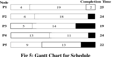
Node Completion Time
4 19 2
6 18
5 14
13 11
9 13
P1
P2
P3
P4
P5
25
24
[image:4.595.318.529.485.658.2]22 24 19
Fig 5: Gantt Chart for Schedule
Consider a schedule S of 10 task Ti, (1≤ i ≤ 12). Let the
completion time of the these task Ti are { 4, 13, 5, 6, 19, 9, 2,
13, 14, 18 } respectively. According to the schedule given in figure 4, the Gantt chart is shown in fig. 5. According to Gantt chart, the makespan value of the given schedule is 25 and therefore the node utilization (individual) for all computing nodes is given as follows:
Putil(N1) = 25/25 = 1.0 Putil(N2) = 24/25 = 0.96
Putil(N3) = 19/25 = 0.76 Putil(N4) = 24/25 = 0.96
Putil(N5) = 22/25 = 1.0
The node utilization (Average) is given as: Pavg = 0.930.
4.1.5
Reproduction
To select the better individual the reproduction is used from a population of large generation. It form a new population of individual by selecting values from the previous population based on their fitness value. The larger value of fitness has more chance to survive in the next generation. For selection of individuals to the population “survival of fittest” mechanism is used. Following steps are taken for the reproduction: Begin
1. For every individual in chromosome Do
2. Calculate fitness value Ft(x) of chromosome.
3. For every individual t the probability of selection is calculated as:
1
/
.
n
t t t
i
SP f x f x
(13)Where n is number of generation.
4. The additive selection probability of chromosome is calculated as:
1
.
ts t
ASP
SP (14)Where t is total no of individuals in the chromosome. 5. Until population size achieved
End.
4.1.6
Crossover
To generate the new string (offspring) for the next generation crossover operation is performed. In crossover operation first 2 parent for crossover are selected and then select a random crossover point and perform crossover operation with a given crossover probability to create the new string. The principle behind crossover is: “by mating 2 individuals with different but desirable features, an offspring is produced which combines both of those features”.
T1 T2 T3 T4 T5 T6 T7 T8 T9 T10 Chromosome 1
Offspring 1
P1 P4 P3 P2 P1 P5 P1 P5 P3 P2
T1 T2 T3 T4 T5 T6 T7 T8 T9 T10
P1 P4 P3 P2 P2 P1 P4 P3 P3 P5
T8 T5
T1 T2 T3 T4 T5 T6 T7 T8 T9 T10 Chromosome 2
P2 P4 P1 P5 P3 P1 P4 P2 P3 P5
T8 T5 Swap Value
Offspring 2 T1
T2 T3 T4 T5 T6 T7 T8 T9 T10
P2 P4 P1 P5 P5 P5 P1 P1 P3 P2
Crossover Point (cp)
Fig 6: Crossover Operator
Fig. 6 Shows the example of crossover operator. We select a random crossover point and also select a random task (say T7) from parent string. And replace the value of task just after crossover point to T7 and vice-versa for both parent string.
4.1.7
Mutation
[image:4.595.70.267.575.675.2]procedures and create a new individual by applying a random variation between arbitrarily selected individuals. The goals with adaptive probabilities of crossover and mutation are to maintain the genetic diversity in the population and prevent the genetic algorithms to converge prematurely to local minima [13]. An example of mutation operator is given in figure 7. We randomly select 2 task and swap their position and corresponding node value is replaced by previous node value.
T1 T2 T3 T4 T5 T6 T7 T8 T9 T10
Parent String
Child String
Exchange Value
P1 P4 P3 P2 P1 P5 P1 P5 P3 P2
T1 T2 T3 T4 T5 T6 T7 T8 T9 T10
[image:5.595.56.275.175.277.2]P1 P1 P3 P2 P1 P5 P5 P5 P3 P2
Fig 7: Mutation Operator
4.1.8
Termination
The algorithm upholds the finest solution found so far in the population since reproduction is used for selection. The algorithm terminates when generations are completed. A fixed or predefined number of generations are used as the stopping condition because the proposed method includes a problem-precise heuristic and it can search the design space in a small number of assessments. The results are obtained by applying the heuristic to the first chromosome. By applying this heuristic to a new set of population differing slightly from the original population for a fixed number of times results in the best solution.
5.
EXPERIMENTAL RESULT AND
DIS-CUSSION
This section describes the experimental results and then these results are analyzed based on different comparison matrix. The performance evaluation of proposed AHGA algorithm and the comparison study with FCFS and HGA algorithms for task scheduling have been done on OMNeT++.
6.
PARAMETERS
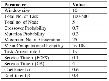
[image:5.595.314.541.343.543.2]The various parameters are used for performance measurem-ent of proposed AHGA algorithm. The value of all parameters with their initial value and their performance matrix in given in table 1.
Table 1. Simulation Parameters
Parameter Value
Window size 10
Total No. of Task 100-500
Total no. of Node 5
Crossover Probability 0.7
Mutation Probability 0.3
Maximum No. of Generation 25
Mean Computational Length χ 5s-10s
Task Arrival rate λ 1s
Service Time τ (FCFS) 0.1
Service Time τ (GA) 4
Coefficient α 0.6
Coefficient β 0.4
All input parameters describe in table 1 read at runtime and are specified in the omnetpp.ini file. The assumption used for simulation environment is given as follows:
The computational length of the task follow the exponential distribution χ.
The arrival pattern of the task follow the Poisson distribution with the arrival rate of λ.
The service time for the task dispatcher is given as τ
6.1
Performance Measurements
To check the accuracy, the proposed algorithm is compare with a well design first-come-first-served and HGA algorithm. The comparison is done for both heterogeneous and homogeneous environment. Five computing nodes are used to simulate the grid system and a set of independent task with no data dependency. For homogeneous scenario the capacity of all computing nodes is taken as 1, since each node has equal capacity while for heterogeneous scenario, two computing nodes are randomly selected and after than we double their capacity.
6.2
Performance under homogeneous
scenario
For homogeneous scenario it is assumed that all the nodes have the equal capability to execute the task and then simulate the algorithm. For simulation, a varying number of tasks are taken and vary the mean computational length χ between 5s to 10s and then analyse the result.
Fig 8: Makespan Value
Fig. 8 show the comparative analysis of makespan value and number of task. The figure shows that as the number of task increase, the value of makespan is also increase. For FCFS algorithm makespan value vary from 150-900.
Table 2. Performance measurement for homogeneous nodes
Total Task Makespan Value AHGA HGA FCFS
100 131.12 136.59 177.49
150 203.74 212.22 275.11
200 270.09 281.34 354.37
250 328.93 342.63 409.52
300 397.01 414.01 530.60
350 505.65 526.72 584.01
400 562.04 585.46 655.60
450 651.07 678.20 744.26
[image:5.595.77.258.586.720.2]Similarly for HGA and AHGA it vary from 800 and 100-700 respectively. The result shows that the proposed AHGA algorithm minimize the makespan value significantly better than FCFS and HGA approach. Table 2 show the performance list of makespan value for homogeneous nodes with variation in mean computational length χ for FCFS, HGA and our AHGA algorithm respectively. We vary the number of task from 100 to 500, and also vary the mean computational length χ from 5s to 10s. The table shows that the proposed AHGA algorithm minimizes makespan value better for each number of tasks.
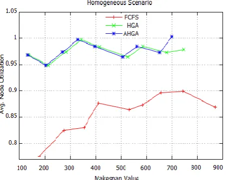
Fig 9: Average Node Utilization
A comparison between average node utilization and number of task is given is fig. 9. As the number of task increase the node utilization very. For HGA and AHGA it remain same up to 450 task and range between 0.95-1. As show in graph as number of task increases than 450 the AHGA maximize the average node utilization value than HGA approach.
Fig 10: Makespan Value Vs. Average Node Utilization
Fig. 10 gives the comparison between makespan value and average node utilization. For FCFS, the node utilization (avg.) initially very low and as the value of makespan increases average node utilization also increase but limited to 0.9. As compare to HGA and AHGA value of average node utilization is same for 450 task but as task value increases AHGA increase the value of average node utilization.
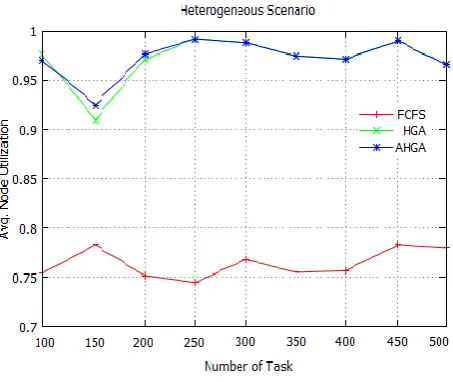
6.2.1 Performance under heterogeneous scenario
For heterogeneous scenario we assume that all computing nodes has its own processing capability and different with each other. For heterogeneous nodes we change the capacity of two randomly selected nodes. For this we double the capacity of selected node as given in homogeneous scenario. To obtain performance matrix, mean computation length is varied between 5s to 10s.
[image:6.595.326.532.275.398.2] [image:6.595.315.544.467.666.2] [image:6.595.55.282.482.663.2]The comparative analysis of makespan value and number of task for heterogeneous nodes is given in fig. 11. The value of makespan increases constantly for the FCFS and lies in the interval [100-800]. As the number of task increase the value of makespan for HGA and AHGA lies between interval [100-500]. The AHGA performed better as compare to FCFS and also provide enhanced and minimized makespan values than HGA.
Table 1. Performance measurement for heterogeneous nodes
Total Task Makespan Value AHGA HGA FCFS
100 93.83 97.06 136.81
150 150.32 159.49 221.77
200 192.67 201.92 302.11
250 236.49 246.35 379.32
300 288.91 294.13 471.33
350 357.01 371.88 536.40
400 407.43 424.41 617.74
450 456.96 476.00 681.67
500 521.16 542.87 768.30
Table 2 show the performance list of makespan value for heterogeneous nodes with variation in mean computational length χ for all three algorithms. The number of task are varied from 100 to 500, and similarly the mean computational length χ is varied from 5s to 10s for every set of task.
Fig 11: Makespan Value
Fig 12: Average Node Utilization
Fig. 13 gives the comparison between makespan value and average node utilization. The result shows that our proposed algorithm work outstanding than FCFS and as compare to HGA, it provide quite better and nearby result.
Fig 13: Makespan Value Vs. Average Node Utilization
7.
CONCLUSION
With the rapid development of technology, grid computing have increasingly becomes an attractive computing platform for a variety of applications. In this paper a hybrid method for job scheduling based on genetic algorithm to schedule the sequential and heterogeneous task for grid computing environment is presented. The performance of proposed method is measured for both homogeneous and heterogeneous scenario and the result shows that proposed AHGA algorithm is improved than first-come-first-served and HGA methods and provide near optimal schedule. The future plan is to perform a broad assortment of experiments to improve the performance, efficiency and integrating our algorithm with existing ideas.
8.
REFERENCES
[1] I. Foster, C. Kesselman, and S. Tuecke, The anatomy of the grid: Enabling scalable virtual organizations, The International Journal of High Performance Computing Applications, 15 (3), 200-222. (2001)
[2] Rajkumar Buyya, and Srikumar Venugopal, A Gentle Introduction to Grid Computing and Technologies, Computer Socity of India, CSI Communication, July (2005).
[3] Albert Y. Zomaya, Yee-Hwei, Observations on Using Genetic Algorithms for Dynamic Load-Balancing, IEEE Transections on Parallel and Distributed System, Vol. 12, No. 9, 899-911. (2001)
[4] Yajun Li, Yuhang Yang, Maode Ma, and Liang Zhoy, A hybrid load balancing strategy of sequential tasks for grid computing environments, Future Generation Computer Systems, 25, 819-828. (2009)
[5] Junwei Cao, Daniel P. Spooner, Stephen A. Jarvis, Graham R. Nudd: Grid load balancing using intelligent agents, Future Generation Computer Systems 21, 135– 149. (2005)
[6] The OMNeT++ Discrete Event Simulation System. http://www.omnetpp.org/. (2012)
[7] OMNeT++ User Manual,
http://www.omnetpp.org/doc/omnetpp/manual/usman.ht ml. (2012)
[8] Albert Y. Zomaya, Chris Ward, and Ben Macey: Genetic Scheduling for Parallel Processor Systems: Comparative Studies and Performance Issues, IEEE Transections on Parallel and Distributed System, Vol. 10, No. 8, 795-812. (1999)
[9] Shanshan Song, 0.6Kai Hwang, and Yu-Kwong Kwok: Risk-Resilient Heu0.4ristics and Genetic Algorithms for Security-Assured Grid Job Scheduling, IEEE Transections on Computers, Vol. 55, No. 6, 703-719. (2008)
[10]K. Q. Yan, S.C. Wang, C.P. Chang, J.S. Lin: A hybrid load balancing policy underlying grid computing environment, Computer Standards & Interfaces 29, 161– 173. (2007)
[11]Kuo-Qin Yan, Shun-Sheng Wang, Shu-Ching Wang, Chiu-Ping Chang: Towards a hybrid load balancing policy in grid computing system, Expert Systems with Applications 36, 12054–12064. (2009)
[12]A. Varga, and R. Hornig, An Overview of the OMNeT++ Simulation Environment. In the Proceedings of First International Conference on Simulation Tools and Techniques for Communications, Networks and Systems (SIMUTools 2008), Marseille, France. (2008)
[13]S.N.Sivanandam, and S.N.Deepa: Introduction to Genetic Algorithm, Springer-India. (2008))
[14]R. L. Haupt, and S. E. Haupt: Practical Genetic Algortihms, John Wiley & Sons. (2004)
[15]INET Framework Documentation,
http://www.omnetpp.org/doc/INET. (2012)
[image:7.595.56.280.339.521.2]