Filtering Function Method for the Cauchy Problem of a Semi Linear Elliptic Equation

(1)

http://dx.doi.org/10.4236/jamp.2015.312184

How to cite this paper: Zhang, H.W. and Zhang, X.J. (2015) Filtering Function Method for the Cauchy Problem of a Semi- Linear Elliptic Equation. Journal of Applied Mathematics and Physics, 3, 1599-1609.

http://dx.doi.org/10.4236/jamp.2015.312184

Filtering Function Method for the Cauchy

Problem of a Semi-Linear Elliptic Equation

Hongwu Zhang

*

_{, Xiaoju Zhang}

School of Mathematics and Information Science, Beifang University of Nationalities, Yinchuan, China

This work is licensed under the Creative Commons Attribution International License (CC BY). http://creativecommons.org/licenses/by/4.0/

Abstract

A Cauchy problem for the semi-linear elliptic equation is investigated. We use a filtering function method to define a regularization solution for this ill-posed problem. The existence, uniqueness and stability of the regularization solution are proven; a convergence estimate of Hölder type for the regularization method is obtained under the a-priori bound assumption for the exact solution. An iterative scheme is proposed to calculate the regularization solution; some numerical results show that this method works well.

Keywords

Ill-Posed Problem, Cauchy Problem, Semi-Linear Elliptic Equation, Filtering Function Method, Convergence Estimate

1. Introduction

Let Ω be a bounded, connected domain in n1

(

1

)

n

− _>

 with a smooth boundary ∂Ω and assume that H is a real Hilbert space. We consider the following Cauchy problem of a semi-linear elliptic partial differential equation

( )

(

( )

)

( )

, , , , , , , 0 ,

, 0, , 0 ,

0, , ,

0, 0, ,

yy x

y

u y x L u y x f y x u y x x y T

u y x x y T

u x x x

u x x

ϕ

 − = ∈ Ω < <



= ∈ ∂Ω ≤ ≤

 

= ∈ Ω



 ₌ _{∈ Ω}



(1.1)

where L_x:D L

( )

_x ⊂H→H denotes a linear densely defined self-adjoint and positive-definite operator with respect to x. The function ϕ is known, and f : × n−1×H→H is an uniform Lipschitz continuous

(2)

function, i.e., existing k>0 independent of w v, ∈H , y∈, x∈n−1 such that

(

, ,

)

(

, ,

)

.

f y x w −f y x v ≤k w v− (1.2) Further, we suppose λ_n

(

n≥1

)

be the eigenvalues of the operator L_x, i.e., for the boundary value problem

in ,

0, on ,

x n n n n

L X X X

λ

= Ω



 ₌ _∂Ω

 (1.3)

there exists a nontrivial solution X_n∈H. And λ_n

(

n≥1

)

satisfy

1 2 3

0 and lim _n .

n

λ λ λ λ

→∞

< ≤ ≤ ≤ = ∞ (1.4)

Our problem is to determine u y

( )

,⋅ from problem (1.1).

Problem (1.1) is severely ill-posed, i.e., a small perturbation in the given Cauchy data may result in a dramatic error on the solution [1]. Thus regularization techniques are required to stabilize numerical computations, (see [1] [2]). We know that, as the right term f =0, it is the Cauchy problem of the homogeneous elliptic equations. For the homogeneous problem, there have many regularization methods to deal with it, (see [3]-[8]). We note that, these references mainly consider the Cauchy problem of linear homogeneous elliptic operator equation, but the literature which involves the semi-linear cases is quite scarce. In 2014, [9] considered the problem (1.1), where the authors used Fourier truncated method to solve it and derived the convergence estimate of logarithmic type. Recently, there are some similar works about the Cauchy problem for nonlinear elliptic equation, and they have been published, such as [10][11].

In the present paper, we adopt a filtering function method to deal with this problem. The idea of this method is similar to the ones in [4][5][12] [13], etc. However, note that our method here is new and different from them in the above references (see Section 2). Meanwhile we will derive the convergence estimate of Hölder type for this method, which is an improvement for the result in [9].

This paper is organized as follows. In Section 2, we use the filtering function method to treat problem (1.1) and prove some well-posed results (the existence, uniqueness and stability for the regularization solution). In Section 3, a Hölder type convergence estimate for the regularized method is derived under an a-priori bound assumption for the exact solution. Numerical results are shown in Section 4. Some conclusions are given in Section 5.

2. Filtering Function Method and Some Well-Posed Results

2.1. Filtering Function Method

We assume there exists a solution to problem (1.1), then it satisfies the following nonlinear integral equation (see [9])

( )

(

)

₀

(

)

( )( )

1

sinh

, cosh _n _n y n _n d _n,

n _n

y

u y x y f u X

λ τ

λ ϕ τ τ

λ

∞

=

 ₋ 

 

= +

 

 

∑

∫

(2.1)

here, X_n are the orthonormal eigenfunctions for the operator L_x, and

( )( )

(

)

, , , , , , ,

n Xn fn u y f y x u y x Xn

ϕ = ϕ = (2.2)

,

⋅ ⋅ is the inner product in H.

From (2.1), we can see that the functions cosh

(

λny

)

, sinh

(

λn

(

y−τ

)

λn tend to infinity (as n→ ∞),

so in order to guarantee the convergence of solution u y x

( )

, , the high frequencies(n→ ∞) of two functions need to be eliminated. Therefore, a natural way is to use a filter function q

(

α λ, n

)

to filter out the high

frequencies of cosh

(

λny

)

, sinh

(

λn

(

y−τ

)

λn and obtain a stable approximate solution, this is so-

called filtering function method.

Let ϕδ be the noisy data, and satisfying

,

δ

(3)

where δ is the error level, ⋅ is the H-norm. According to the above description, for r>0, we choose the filter function q

(

α λ, _n

)

=1 1

(

+αcosh

(

λ_n

(

T+r

)

, and define the following regularization solution

( )

(

)

(

)

(

)

(

)

(

)

( )

(

)

(

)

(

)

1

0

cosh ,

1 cosh

sinh

d ,

1 cosh

n n

n

n n

y

n

n n

y

u y x

T r

y f u

X

T r

δ δ

α

δ α

λ ϕ

α λ

λ τ τ

τ

λ α λ

∞

=

  =

 + +





− _

+ _

+ + 



∑

∫

(2.4)

where, ϕ_nδ = ϕδ,X_n , fn

( )

u

( )

y f y x u

(

, ,

( )

y x,

)

,Xn

δ δ

α = α .

In fact, it can be verified that (2.4) satisfies the following mixed boundary value problem formally

( )

(

)

(

)

( )

(

)

(

)

( )

1

, , , , 0 ,

1 cosh

, 0, , 0 ,

0, , ,

1 cosh

0, 0, .

n

x n

yy

n

n n

n

y

f u y

u y x L u y x X x y T r

T r

u y x x y T r

u x X x

T r

u x x

δ α

δ δ

α α

δ α

δ δ

α

δ α

α λ

ϕ

α λ

∞

=

∞

=



 − = ∈Ω < < +

 + +



 = ∈∂Ω ≤ ≤ +

 

 ₌ _∈Ω

 ₊ ₊



 ₌ _∈Ω



∑

(2.5)

Our idea is to approximate the exact solution (2.1) by the regularization solution (2.4), i.e., using the solution of (2.5) to approximate the one of (1.1).

2.2. Some Well-Posed Results

Let 0< <α 1, x>0, for the fixed 0≤ ≤ ≤ +

τ

y T r, we define the function

(

)

2e( ₍) ₎

, , ,

2 e

y x T r x

h y x

τ

α

−

+

=

+ (2.6)

then h y

(

, ,τ x

)

attain unique maximum at the point x₀, and from

(

y−τ

)

≤ +T r,

(

T+ −r

) (

y−τ

)

≤ +T r, we have

(

) (

)

(

)

(

) (

)

(

) (

)

1 0

1

, , , , 2

2

2 ,

y

y y

T r

T r T r

y y

T r T r

h y x h y x y T r y

T r

T r T r

T r

τ

τ τ

τ τ τ τ α

α α

−

− ₋ − ₋

+

+ +

− −

− ₋ − ₋ ₋

+ +

≤ = − + − −

+

≤ + + =

+

(2.7)

note that, when τ=0, it can be obtained that

(

,

)

2 .

y T r

h y x ≤ α− + (2.8) Now, we prove that the problem (2.4) is well-posed (existence, uniqueness and stability for the regularization solution), the proof mentality of Theorem 2.1 mainly comes from the references [14], which describes the existence and uniqueness for the solution of (2.4).

Theorem 2.1. Let ϕδ∈H, f satisfies (1.2), then the problem (2.4) exists a unique solution

[

]

(

0, ;

)

uαδ∈C T+r H .

(4)

( )( )

(

)

(

)

(

)

(

)

(

)

( )( )

(

)

(

)

(

)

1 0 cosh , 1 cosh sinh d , 1 cosh n n n n n n y n n n y

G w y

T r

y f w

X T r ∞ =   ⋅ =  + +   − _ + _ + +  

∑

∫

δ λ ϕ α λ

λ τ τ

τ

λ α λ

(2.9)

then for w v, ∈C

(

[

0,T+r

]

;H

)

, p≥1, we can prove the following estimate is valid

( )( )

,

( )( )

,

(

)

! p

p p kC T r

G w y G v y w v

p

α +

⋅ − ⋅ ≤ − (2.10)

where

1

2

C_α

λ α

= , ⋅ denotes the sup norm in C

(

[

0,T+r

]

;H

)

.

For p≥1, we firstly use the induction principle to prove

( )( )

,

( )( ) (

,

)

2

(

)

2 .

!

p p

p

p p y T r

G w y G v y kC w v p

α

+

⋅ − ⋅ ≤ − (2.11)

Note that, for 0< <α 1, from (2.7), h y

(

, ,τ x

)

≤2α. Meanwhile, use the basic inequalities

(

)

(

)

( )

cosh e nT r 2

n T r λ

λ ₊ _≥ +

, cosh

(

)

e ny

ny λ

λ ≤ , and sinh

(

)

e n(y )

n y

λ τ

λ ₋τ _≤ −

. When p=1, from (2.9), (1.2), we have

( )( )

(

)

(

)

(

)

(

)

(

)

(

( )( )

)

(

)

(

)

(

)

(

)

(

)

(

( )( )

)

( ) ( )

(

)

(

( )( )

)

( )( )

(

)

2 2 0 1 2 0 1 2 2 0 0 1 1 2 2 0 1 1 , , sinh d 1 cosh sinh d 1 cosh 2e d d 2 e 2 n n n y

n n n

n n n n y n n n n n y y y n n T r n y n n n

G w y G v y

y

f w f v X

T r

y

f w f v

T r

f w f v

y f w f v

τ λ

λ

λ τ

τ τ τ

λ α λ

λ τ

τ τ τ

λ α λ

τ τ τ τ

λ α τ τ λ α ∞ = ∞ = − ∞ + = ∞ = ⋅ − ⋅ − = − + +  ₋    ≤ _ − _ + +         ≤ _ _ − +       ≤ _ _ −  

∑∫

∑ ∫

∑∫

∫

∑

∫

(

)

(

( )

)

(

( )

)

(

)

(

)

2 2 0 1 2 2 2 0 1 2 2 2 d 2

, , , , , , d

2

d

. y

y

T r f w f v

k T r w v

k C y T_α r w v

τ

τ τ τ τ τ

λ α τ λ α   ≤ + _ _ ⋅ ⋅ − ⋅ ⋅     ≤ + _ _ −   ≤ + −

∫

When p=i, we suppose

( )( )

2

(

)

2

(

)

2

, , ,

! i i i

i i y T r

G w y G v y kC w v

i

α

+

(5)

then for p= +i 1, by (2.12), it similarly can be proven that

( )( )

(

)

(

)

(

)

(

)

(

)

(

( )

)

( )

(

( )

)

( )

)

(

)

(

)

(

)

(

)

(

)

(

( )

)

( )

(

( )

)

( )

)

( )

(

)

( )

(

( )

)

( )

(

)

(

)

( )( )

2

1 1

2 0

1

2 0

1

2

2 0

1 1

2 2

0 1

, ,

sinh

d

1 cosh

sinh

d

1 cosh

2

d

2

, ,

i i

n

y _i _i

n n n

n

n n

n

y _i _i

n n

n

n n

y _i _i

n n

n

y _i _i

G w y G v y y

f G w f G v X T r

y

f G w f G v T r

y f G w f G v

k T r G w G v

λ τ

τ τ τ

λ α λ

λ τ

τ τ τ

λ α λ

τ τ τ

λ α

τ τ

λ α

+ +

∞

=

∞

=

∞

=

⋅ − ⋅

−

= −

+ +

 ₋ 

 

≤ _ − _

+ +

 

 

 

≤ _ _ −

 

 

≤ + _ _ ⋅ − ⋅

 

∑∫

∑ ∫

∑

∫

(

)

(

)

(

)

(

)

₍

(

₎

)

2 2

2

0 1

1 1

2 2 2

d

2

| | d

!

. 1 !

i y i _i i

i i

T r

k T r kC w v i

y T r

kC w v

i

α

τ

τ τ

λ α

+ +

+

  +

≤ + _ _ −

 

+

≤ −

+

∫

By the induction principle, we can obtain that

( )( )

,

( )( ) (

,

)

2

(

)

2 ,

!

p p

p

p p y T r

G w y G v y kC w v p

α

+

⋅ − ⋅ ≤ − (2.13)

hence, it is clear that

( )( )

,

( )( )

,

(

)

.

! p

p p kC T r

G w y G v y w v

p

α +

⋅ − ⋅ ≤ − (2.14)

We consider G C:

(

[

0,T+r

]

;H

)

→C

(

[

0,T+r

]

;H

)

, and from real analysis, we know

(

)

(

)

lim 0.

! p

p

kC T r

p

α →∞

+

= (2.15)

There must exist a positive integer number p₀, such that

(

)

0

0 1

! p

kC T p

α

< < , therefore _Gp0_{is a contraction,}

it shows that the equation _Gp0

( )

_w =_w_{has a unique solution} _uδ _C

(

[

_0,_T _r

]

_;_H

)

α∈ + . Noting that

( )

(

p0

)

( )

G G u_αδ =G u_αδ , thus, _Gp0

(

_{G u}

( )

δ

)

_{G u}

( )

δ

α = α . By the uniqueness of the fixed point of Gp0, we have

( )

G uαδ =uαδ, so the equation G w

( )

=w has a unique solution uαδ ∈C

(

[

0,T+r

]

;H

)

. □

In the following, we give and prove the stability of the regularization solution. Theorem 2.2 Suppose f satisfies (1.2), uαδ₁ and u 2

δ

α be the solutions of problem (2.4) corresponding to the

measured datum ϕ₁δ and ϕ₂δ, respectively, then for 0< ≤ +y T r, we have

( )

1 , 2 , 1 1 2 ,

y T r

(6)

where

(

)

( ) 2 1 8 2 1 1 8

8 1 e

k T r y

k T r y

C λ λ +  ₊    = +     .

Proof. From (2.4), we have

( )

(

)

(

)

(

)

(

)

(

( )

)

1, 1 1 ₀ 1 cosh sinh d ,

1 cosh 1 cosh

n n y n n

n n

n n n

y y f u

u y X

T r T r

δ δ

α δ

α

λ ϕ λ τ τ

τ

α λ λ α λ

∞ =  ₋    = _ + _ + + + +    

∑

∫

(2.17)

( )

(

)

(

)

(

)

(

)

( )

(

( )

)

2, 2 2 ₀ 1 cosh sinh d ,

1 cosh 1 cosh

n n y n n

n

n _n

n n

y y f u

u y X

T r T r

δ δ

α δ

α

λ ϕ λ τ τ

τ

α λ λ α λ

∞ =  ₋    = _ + _ + + + +    

∑

∫

(2.18)

where ϕ_{i n}δ_, = ϕ_iδ,X_n , i=1, 2.

By (2.17), (2.18), (2.7), (2.8) and (1.2), we have

( )

(

)

(

)

(

)

(

)

(

)

(

( )

(

( )

(

)

( )

)

( )

)

(

)

(

)

(

)

(

)

(

)

(

)

(

)

(

)

(

)

(

)

(

( )

)

2 1 2 2 1 2 1, 2, 0 1 2 1, 2, 1 1 2 0 1 , , sinh cosh d

1 cosh 1 cosh

cosh 2 1 cosh sinh 2 d 1 cosh

n n n

n n n y

n

n _n

n n

n

n n n n n n y n n n n n

u y u y

y f u f u y

X

T r T r

y

X T r

y

f u f u X T r ∞ = ∞ = ∞ = ⋅ − ⋅  ₋ ₋ ₋    = _ + _ + + + +     ≤ − + + − + − + +

∑

∫

∑

∑∫

δ δ α α δ δ δ δ α α δ δ δ δ α α

λ τ τ τ

λ ϕ ϕ

τ

α λ λ α λ

λ

ϕ ϕ

α λ

λ τ

τ τ τ

λ α λ

( )

(

)

( ) ( )

(

( )

)

(

)

( )

(

( )

)

2 2 2 2 2

1, 2, ₀ 1 2

1 1 1

2 2

1, 2, ₀ 1 2

1 1 1

2 2 2

2

1 2 ₀

1

2e 2e

2 2 d

2 e 2 e

8 8 d

8 8 n n n n n y y y

n n n n

T r T r

n n

y y

y

T r T r

n n n n

n n

y y

y

T r T r

y

f u f u y

f u f u k y − ∞ ∞ + + = = − ∞ ∞ − − + + = = − − + +     ≤ _ _ − + _ _ − + +     ≤ − + − ≤ − +

∑

∑∫

∑

∑∫

∫

λ λ τ

δ δ δ δ

α α

λ λ

τ

δ δ δ δ

α α

δ δ

ϕ ϕ τ τ τ

λ

α α

α ϕ ϕ α τ τ τ

λ

α ϕ ϕ α

λ

( )

2

2 1 , 2 , d . T r+ _u ⋅ −_u ⋅

τ

δ δ

α α

α τ τ τ

Subsequently,

( )

2

(

)

( )

2 2

2 2 2

1 2 1, 2, ₀ 1 2

1

, , 8 8 , , d ,

y

T r T r

n n

k T r

u y u y u u

τ

δ δ δ δ δ δ

α α α α

α ϕ ϕ α τ τ τ

λ

+ _{⋅ −} _⋅ _≤ ₋ ₊ +

∫

+ _{⋅ −} _⋅

using Gronwall’s inequality [15], we have

( )

(

)

( ) 2 1 8 2 2 2 2

1 2 1, 2,

1

8

, , 8 1 e ,

k T r y y

T r

n n

k T r y

uαδ y uαδ y λ δ δ

α ϕ ϕ

λ + +  ₊    ⋅ − ⋅ ≤ + −     (2.19)

then from the above inequality (2.19), the stability result (2.16) can be obtained. □

3. Convergence Estimate

In this section, under an a-priori bound assumption for the exact solution a convergence estimate of Hölder type for the regularization method is derived. The corresponding result is shown in Theorem 3.1.

(7)

(2.3). If the exact solution u satisfies

( )

_{( )}

2

2 2

1

e nT r y , , ,

n n

u y X E

λ ∞

+ −

=

⋅ ≤

∑

(3.1)

and the regularization parameter α is chosen as ,

α δ= (3.2)

then for fixed 0< ≤y T, we have the following convergence estimate

( ) ( )

1

, , ,

y T r

u_αδ y⋅ −u y ⋅ ≤Cδ − + (3.3)

here C=C₁+C₂,

2 1 8 2 2 2 1 8 8 1 k Ty k Ty

C E ye λ

λ     = +    

, C₁ is given in Theorem 2.2.

Proof. Denote u_α be the solution of problem (2.4) with exact data ϕ. We know that .

uαδ −u ≤ uαδ −uα + uα−u (3.4)

From Theorem 2.2, for 0< ≤y T, we have

( )

,

( )

, 1 .

y T r

u_αδ y⋅ −u_α y⋅ ≤Cα− + ϕδ −ϕ (3.5) By (2.1), (2.4), (2.7), (2.8), we have

( ) ( )

(

)

(

)

(

)

(

)

(

)

(

)

( )( )

(

)

(

)

(

( )( )

)

(

)

(

)

(

)

(

)

(

)

(

)

(

)

(

)

(

)

( )( )

2 2 0 =1 2 0 =1 2 0 =1 , , cosh sinh

2 cosh d

1 cosh

sin

2 d

1 cosh

cosh sinh

2 cosh d

1 cosh

n y n n

n n n

n _n _n

n n n

y

n n

n y n n

n n

n _n

n

u y u y

T r y f u

y X

T r

y f u f u

X T r

T r y f u

y T r ∞ ∞ ∞ ⋅ − ⋅   + −   ≤ +   + + _ _ − − + + +  ₊   ₋    ≤ +  ₊ ₊     

∑

∫

∑∫

∑

∫

α α

α λ λ τ τ

λ ϕ τ

λ

α λ

λ τ τ τ

τ

λ α λ

α λ λ τ τ

λ ϕ τ

λ α λ

(

)

(

)

(

)

(

)

(

)

(

( )( )

)

(

)

(

)

(

)

(

)

(

)

(

)

( )( )

(

)

(

)

(

)

(

)

(

)

(

( )( )

)

2 2 0 =1 2 2 0 =1 2 2 0 0 =1 sinh 2 d 1 cosh cosh sinh

2 cosh d

1 cosh sinh 2 d 1 cosh n y n n n n n

n y n n

n n n _n n n y y n n n n n y

f u f u T r

T r y f u

y T r

y

d f u f u

T r ∞ ∞ ∞      ₋    + _ − _ + +      ₊   ₋      ≤ +  ₊ ₊         ₋    + _ _ − + +    

∑ ∫

∑

∫

∑∫ ∫

α α λ τ

τ τ τ

λ α λ

α λ λ τ τ

λ ϕ τ

λ

α λ

λ τ

τ τ τ τ

λ α λ

( ) ( )

_{( )}

( ) ( )

( )( )

(

)

( ) ( )

2 2 2 2 2 0 0

=1 1 =1

2 2( )

2 2 2

0

=1 1

2 2 2

0 1

2 e 1 2e

2 e , , 2 d d

2 e 2 e

8 8 d

8 8 , ,

n n

n

n n

y y

y y T r y

n n n

T r T r

n n

y y

y

T r T r

n n

n

y y

y T r T r T r

u y X f u f u

y

E f u f u

y

E k u u

− ∞ ∞ + − + + − − ∞ − + + − − + + +     ≤ _ _ ⋅ + _ _ − + +     ≤ + − ≤ + ⋅ − ⋅

∑

∑∫ ∫

∑

∫

λ λ τ

λ α λ λ τ α τ α

α _τ _τ _τ _τ

λ

α α

α α α τ τ τ

λ

α α α α τ τ

λ

2

(8)

For 0≤ ≤y T, we get

( ) ( )

2 2 2

2 ₂ ₂ 2

0 1

, , 8 8 , , d ,

y

T r _u _y _{u y} _E k T T r _u _u

τ

α α

α α α τ τ τ

λ

+ _{⋅ −} _⋅ _≤ ₊

∫

+ _{⋅ −} _⋅ _(3.6)

use Gronwall’s inequality [15], it can be obtained that

( ) ( )

2 1

8

2 2

2 ₂ ₂

1

8

, , 8 1 e ,

k Ty y

T r _u _y _{u y} _E k Ty λ

α

α α

λ

+

 

 

⋅ − ⋅ ≤ +

 

 

thus

( ) ( )

1

2

, , .

y T r

u_α y⋅ −u y⋅ ≤Cα − + (3.7) From (3.2), (3.4), (3.5), (3.7) and (2.3), we can obtain the convergence result (3.3). □

4. Numerical Experiments

In this section, we verify the accuracy and efficiency of our given regularization method by the following numerical example

( )

(

)

cos , , 0 π, 0 1,

0, , 0 π,

0, 0, 0 π,

, 0 ,π 0, 0 1,

yy xx y

u u u g y x x y

u x x x

u x x

u y u y y

ϕ

 + = + < < < <

 ₌ _{≤ ≤}



 ₌ _{≤ ≤}



 ₌ ₌ _{≤ ≤}



(4.1)

here we take Ω =

( )

0,π , H=L2

( )

0,π ,

2 2

x

L x

∂ = −

∂ , then

2 n n

λ = and

( )

2sin

( )

π n

X x = nx .

It is clear that

(

)

(

)

(

2

)

, π 2

u y x =x x− +y is an exact solution of problem (4.1), thus

( )

(

)

(

2

)

(

)

(

2

)

, 2 π 2 2 cos π 2

g y x = x x− + +y − x x− +y , ϕ

( )

x =u

( )

0,x =2x x

(

−π

)

. We choose the measured data as ϕδ

( )

x =ϕ

( )

x

(

1+ε

(

x 2 1−

)

, where ε is an error level, and

( )

2

1 2 2 0

π

: .

N

ii ii L

ii

x x N

δ δ

δ ϕ ϕ ϕ ϕ

=

 

= − =_ − _



∑

 (4.2)

Let 0=y₀<y₁<<yµ<<y_M =1 for

µ

=0,1, 2,,M , the regularization solution uαδ

(

yµ,x

)

with

y M

µ =

µ

can be computed by the following iteration scheme

(

,

)

( )

1, sin

( )

2, sin 2

( )

m, sin

( )

,

uαδ yµ x =vµ x =wµ x +w µ x ++w µ mx (4.3)

here

(

)

(

,

)

,

1 cosh 1

j j

a w

j r

µ

µ = ₊_α ₊ , and

( )

(

)

(

( )

)

( )

)

( )

(

)

(

)

(

( )

)

( )

)

( )

(

)

(

)

(

( )

)

( )

)

( )

(

)

(

)

(

( )

)

( )

)

( )

1 1

2 2 1 1

π

, ₀ 1

π

2 0

π

1 0

π

0 0 0

2

cosh sinh cos , sin d d

π 2

sinh cos , sin d d

π 2

sinh cos , sin d d

π 2

sinh cos , sin d d ,

π

y

j j _y

y

a jy j y v x g x jx x

j

j y v x g x jx x

j

j y v x g x jx x

j

j y v x g x jx x

j

µ

δ

µ µ µ µ

µ µ

µ

ϕ τ τ τ

τ τ τ

−

= + − +

+ − +

+ + − +

+ − +

∫ ∫



(9)

( )

(

)

π

( ) ( )

0 ₀

2

1 2 1 , sin d .

π

j

v x =ϕδ x =ϕ x +ε x − ϕδ =

∫

ϕδ x jx x (4.5)

For a fixed 0< ≤y 1, in order to make the sensitivity analysis for numerical results, we define the relative root mean square error between the exact and approximate solutions as

( )

(

)

(

)

(

)

(

)

2 0

1

, ,

. 1

, N

ii ii

ii N

ii ii

u y x u y x

N u

u y x N

δ α

ε =

=

−

=

∑

(4.6)

We adopt the above given algorithms to compute the regularization solution at y M

µ =

µ

with M =50,

for

µ

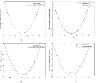
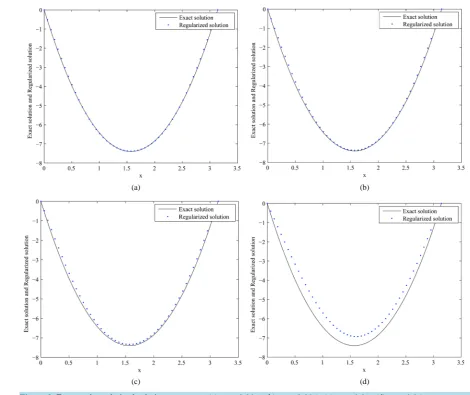
=1, 2,,M j, =1,,m=4. Taking r=0.5, for ε=0.001, 0.005, 0.01, 0.05, the numerical results for u y

( )

,⋅ and u_αδ

( )

y,⋅ at y=0.6,1,

(

µ=30, 50

)

are shown in Figure 1 and Figure 2, respectively. For

0.00001, 0.0001, 0.001, 0.01, 0.05

ε= , the relative root mean square errors for the various error levels ε and

regularization parameters α at y=0.6,1 are shown in Table 1. In the computational procedure, the regularization parameter α is chosen by (3.2), and α δ= is computed by (4.2).

From Figure 1 and Figure 2 and Table 1, it can be observed that our regularization method is effective and stable. Meanwhile we note that the smaller ε is, the better the calculation effect is. Table 1 shows that the numerical results become worse when y approaches to 1, which is a common phenomenon in the computation of ill-posed Cauchy problems for the elliptic equation.

(a) (b)

[image:9.595.117.515.355.700.2]

(c) (d)

(10)

(a) (b)

[image:10.595.67.538.80.475.2]

(c) (d)

Figure 2. Exact and regularized solutions at y=1. (a) ε =0.001; (b) ε =0.005; (c) ε =0.01; (d) ε =0.05.

Table 1. The relative root mean square errors for various ε and the regularization parameters α at y=0.6,1.

ε 0.00001 0.0001 0.001 0.01 0.05

α 1 8303e−06 1 8303e−05 1 8303e−04 0 0018 0 0092

( )

0.6 u

ε 0 0087 0 0088 0 0094 0 0284 0 1036

( )

1 u

ε 0 0094 0 0095 0 0105 0 0290 0 1111

5. Conclusion

We use a filtering function method to solve a Cauchy problem for semi-linear elliptic equation. The results of the well-posedness for the approximation problem are given. Under the a-priori bound assumption, the convergence estimate of Hölder type has been derived. Finally, we compute the regularization solution by constructing an iterative scheme. Some numerical results show that this method is stable and feasible.

Acknowledgements

[image:10.595.86.540.513.585.2]

(11)

2015JBK423), NFPBP (2014QZP02) of Beifang University of Nationalities, the SRP of Ningxia Higher School (NGY20140149) and SRP of State Ethnic Affairs Commission of China (14BFZ004).

References

[1] Kirsch, A. (1996) An Introduction to the Mathematical Theory of Inverse Problems. Applied Mathematical Sciences, Vol. 120, Springer-Verlag, New York. http://dx.doi.org/10.1007/978-1-4612-5338-9

[2] Engl, H.W., Hanke, M. and Neubauer, A. (1996) Regularization of Inverse Problems. Mathematics and Its Applica-tions, Vol. 375, Kluwer Academic Publishers Group, Dordrecht. http://dx.doi.org/10.1007/978-94-009-1740-8

[3] Belgacem, F.B. (2007) Why Is the Cauchy Problem Severely Ill-Posed? Inverse Problems, 23, 823.

http://dx.doi.org/10.1088/0266-5611/23/2/020

[4] Feng, X.L., Ning, W.T. and Qian, Z. (2014) A Quasi-Boundary-Value Method for a Cauchy Problem of an Elliptic Equation in Multiple Dimensions. Inverse Problems in Science and Engineering, 22, 1045-1061.

http://dx.doi.org/10.1080/17415977.2013.850683

[5] Hào, D.N., Duc, N.V. and Lesnic, D. (2009) A Non-Local Boundary Value Problem Method for the Cauchy Problem for Elliptic Equations. Inverse Problems, 25, Article ID: 055002. http://dx.doi.org/10.1088/0266-5611/25/5/055002

[6] Hào, D.N., Van, T.D. and Gorenflo, R. (1992) Towards the Cauchy Problem for the Laplace Equation. Partial Diffe-rential Equations, 111.

[7] Isakov, V. (2006) Inverse Problems for Partial Differential Equations. Springer Verlag, Berlin.

[8] Lavrentiev, M.M., Romanov, V.G. and Shishatski, S.P. (1986) Ill-Posed Problems of Mathematical Physics and Anal-ysis. Translations of Mathematical Monographs, Vol. 64, American Mathematical Society, Providence.

[9] Zhang, H.W. and Wei, T. (2014) A Fourier Truncated Regularization Method for a Cauchy Problem of a Semi-Linear Elliptic Equation. Journal of Inverse and Ill-Posed Problems, 22, 143-168. http://dx.doi.org/10.1515/jip-2011-0035

[10] Tuan, N.H., Thang, L.D. and Khoa, V.A. (2015) A Modified Integral Equation Method of the Nonlinear Elliptic Equa-tion with Globally and Locally Lipschitz Source. Applied Mathematics and ComputaEqua-tion, 265, 245-265.

http://dx.doi.org/10.1016/j.amc.2015.03.115

[11] Tuan, N.H. and Tran, B.T. (2014) A Regularization Method for the Elliptic Equation with Inhomogeneous Source. ISRN Mathematical Analysis, 2014, Article ID: 525636.

[12] Clark, G.W. and Oppenheimer, S.F. (1994) Quasireversibility Methods for Non-Well-Posed Problems. Electronic Journal of Differential Equations, 1994, 9 p.

[13] Xiong, X.T. (2010) A Regularization Method for a Cauchy Problem of the Helmholtz Equation. Journal of Computa-tional and Applied Mathematics, 233, 1723-1732. http://dx.doi.org/10.1016/j.cam.2009.09.001

[14] Tuan, N.H. and Trong, D.D. (2010) A Nonlinear Parabolic Equation Backward in Time: Regularization with New Er-ror Estimates. Nonlinear Analysis: Theory, Methods and Applications, 73, 1842-1852.