DOI 10.1007/s40435-014-0081-x
Analysis of vibration suppression of master structure in nonlinear
systems using nonlinear delayed absorber
Yueli Chen · Kwok-wai Chung · Jian Xu · Yixia Sun
Received: 6 December 2013 / Revised: 6 February 2014 / Accepted: 28 February 2014 / Published online: 20 March 2014 © Springer-Verlag Berlin Heidelberg 2014
Abstract In this paper, a nonlinear delayed absorber is pro-posed by a delayed feedback loop and is utilized to absorb or suppress the vibration of a two-degree-of-freedom non-linear system when the primary resonance and the 1:1 inter-nal resonance occur simultaneously. To explain ainter-nalytically mechanism of performance of the absorber, an integral equa-tion method is provided to obtain the second order approx-imation and the amplitude equations. As a result, the feed-back gain and time delay which make the amplitude of the main system equal to zero can be derived analytically. Opti-mal working conditions of the system are extracted from the time delay-response curves, the force-response curves and the frequency-response curves. In the illustrative example, the appropriate choice of feedback gains and time delays can reduce the amplitude of the main system by more than 98 % in comparison with the amplitude with no time delay. All analytical predictions are in excellent agreement with the numerical simulations.
Keywords Delayed differential equation·Nonlinear vibration·Nonlinear delayed absorber·Nonlinear state feedback·Integral equation method
Y. Chen·J. Xu·Y. Sun
School of Aerospace Engineering and Applied Mechanics, Tongji University , Shanghai 200092, People’s Republic of China e-mail: [email protected]
J. Xu
e-mail: [email protected] K. Chung (
B
)Department of Mathematics, City University of Hong Kong, Kowloon, Hong Kong, People’s Republic of China e-mail: [email protected]
1 Introduction
From the viewpoint of engineering, the active control of mechanical and structural vibrations is superior to the pas-sive control in many aspects. However, the presence of unavoidable time delays in controllers and actuators may induce complex dynamic behavior such as undesirable bifur-cations, large-amplitude vibrations, quasi-periodic motions and chaotic behavior etc. It limits the performance of the active control.
Over the past few decades, the controlled systems using time delay have received much attention. Among the pre-vious works, the stability which has arisen from delay has attracted special interest. For example, the Hopf bifurcation of an autonomous difference-differential equation was inves-tigated in [1]. In [2], the case of multi-delayed differential equations was extended from the former work [1] by Belair and Campbell. Stépán and Haller [3] investigated the quasi-periodic oscillations of a delayed robot system and demon-strated that a codimension two Hopf bifurcation occurred for an infinite set of parameter values. Reddy et al. [4] demon-strated that time delay can induce amplitude death of the cou-pled limit cycle oscillators. The dynamics of two coucou-pled van der Pol oscillators with delay coupling was investigated by Wirkus and Rand [5]. They focused on the bifurcation accom-panying the change in number and stability of solutions. In [6], we studied a van der Pol-Duffing oscillator with time delayed position feedback and found two routes to chaos, namely period-doubling cascade and torus breaking.
Time delayed feedback control has been employed to sup-press the dangerous vibrations of nonlinear systems. Hu et al. [7] investigated the primary resonance and the 1/3 sub-harmonic resonance of a Duffing oscillator under linear state feedback control with a time delay. They demonstrated that the appropriate choice of the feedback gains and the time
delay can enhance the performance of vibration suppres-sion. Maccari [8] studied the parametric resonance of the van der Pol oscillator with a time delay state feedback and found that proper choices for the feedback gains and time delay can exclude the possibility of quasi-periodic motion and reduce the amplitude peak of the parametric resonance. Siewe et al. [9] investigated the principal parametric reso-nance of a Rayleigh–Duffing oscillator with time-delayed feedback position and linear velocity terms. It was shown that the proper choice of time delay can broaden the stable region of the non-trivial steady-state solutions and enhance the control performance. El-Gohary and El-Ganaini [10] con-sidered the vibration suppression of a dynamical system to multi-parametric excitations via time-delay absorber. They demonstrated that time delay absorber is effective like ordi-nary one within a specified range of time delay, which is an important factor in selecting the absorber. Leung et al. [11] studied the steady state bifurcation of a periodically excited system under three kinds of delayed feedback controls. They indicated that different feedback gains not only change the bifurcating curves but also can eliminate the saddle-node bifurcation under resonant response. Zhao and Xu [12] inves-tigated the effects of linear delayed feedback control on a nonlinear vibration absorber system. It was shown that the feedback gains and the time delays not only suppress the vibration but also induce complex behaviors, such as quasi-periodic motions and chaotic motions.
In this paper, we investigate a two-degree-of-freedom sys-tem with external excitation. Here, a called nonlinear delayed absorber is proposed to suppress the vibration of the main sys-tem. The integral equation method, which was introduced by Schimidt and Tondl [14] for the case without the time delay, is extended to obtain the second order approximation and the amplitude equations. For some parametrically excited and periodically forced systems, Chen and Xu [15] demonstrated that the accuracy of the analytical solutions obtained from the integral equation method is much higher than that from the method of multiple scales. The feedback gain and time delay which make the amplitude of the main system equal to zero can be derived analytically. Optimal working conditions of the system are extracted from the time delay-response curves, the force-response curves and the frequency-response curves. The appropriate choice of the feedback gain and time delay can suppress the vibration of the main system drastically. Numerical simulations are presented to validate the analyti-cal predictions. It is found that they are in good agreement. 2 Mathematical modeling
Although the effects of time delayed feedback control on the vibration suppression of various nonlinear systems have been widely studied, most papers are concerned with the linear case [7–10,12,13,16]. However, the works on nonlinear time
2 m 1 m 2 c 1 c 1 1 f =k x 1 x 2 x 3 1( ) g x t−
τ
3 2 2 3f
=
k x
+
k x
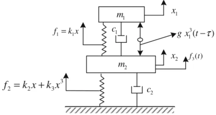
3( ) f tFig. 1 The model describing the nonlinear state feedback control system
delayed feedback control are relatively rare and they focused on the single degree of freedom [11,17]. It is well known that the appropriate choice of feedback gains and time delays can enhance the performance of vibration reduction. Motivated by this advantage, we investigate the vibration suppression by a called nonlinear delayed absorber as shown in Fig.1.
In Fig.1, the system consists of a slave massm1and the
main system m2. The parametersc1 andc2 represent the
damping coefficients of the controller and the main system, respectively. The spring f1is assumed to be linear with the
stiffnessk1 while the spring f2is considered to be
nonlin-ear with force–displacement(f2−x)relationship given as
f2 = k2x+k3x3. The main system is excited by the
peri-odic excitation f3(t) = fsin(ωt). The nonlinear delayed
absorber is composed of a nonlinear delayed feedback loop or controlgx13(t−τ)and the slave massm1. Such control
can be realized by a servo motor and a charge amplifier. The servo motor is activated by the feedback signals derived from measurement of the slave system. The signals are coded to be any desired signals (including nonlinear signals) and actively to drive actions of a controlled beams in an actively delayed format. The controlled beam is connected to the main systemm2 at one end and to the slave massm1at another
end. The charge amplifier is used to enlarge the feedback signals forward to the servo motor and then the gain can be obtained. Thus, the nonlinear delayed absorber is coupled into the system under consideration.The governing equations of the structure shown in Fig.1are given by
m1x¨1+k1(x1−x2)+c1(x˙1− ˙x2)+gx13(t−τ)=0,
m2x¨2+k2x2+c2x˙2+k1(x2−x1)+c1(x˙2− ˙x1)
+k3x32−gx13(t−τ)= f sin(ωt).
(1)
By introducing the following dimensionless time and new parameters t∗= Ωωt, τ∗= Ωωτ, y1= x1xc, y2= x2xc, ω21= k1Ω2 m1ω2, ω2 2= k2Ω2 m2ω2, ζ1= c1Ω m1ω, ζ2= c2Ω m2 ω, α1= k3Ω2xc2 m2ω2 , γ =m1, g∗= gΩ2x2c 1ω , F = fΩ2 ω , (2)
Equation (1) can be written as ¨ y1+ω12(y1−y2)+ζ1(y˙1− ˙y2)+g∗y13(t−τ)=0, ¨ y2+ω22y2+ζ2y˙2+γ ω21(y2−y1)+γ ζ1(y˙2− ˙y1) +α1y32−γg∗y13(t−τ)=Fsin(Ωt). (3)
Here, for simplicity, we drop the ‘∗’ oft∗andτ∗.
3 The integral equation method
Vibrations of various kinds with time delay can be governed by delay differential equations of the form
¨
xi +λixi =φi(xi,x˙i,xiτ,x˙iτ,xj,x˙j,xjτ,x˙jτ;εp,t)
=φi[t],i,j =1,2, . . . . (4) wherexiτ =xi(t−τ)andεpis a parameter.
Theorem 1 Every periodic solution of the differential equa-tion(4)is a solution of the integro-differential equation(see [14]) xi(t)= 2π 0 Gi[t, σ]φi[σ]dσ+ δ n2i λi(ricosnit+ sisinnit) (5) where Gi[t, σ] = π1(21λi + ∞ j=1 cosj(t−σ) ϑλi−j2 )is the
corre-spondingGeneralized Green’s function.
And ifλi =n2i (ni beingan integer) (the resonance case), the parameters ri, si are to be determined by the periodicity equations(see[14]) ri = π1 2π 0 xi(t)cosnitdt si = π1 2π 0 xi(t)sinnitdt (6)
which are equivalent to
2π 0 φi[t]cosnitdt = 2π 0 φi[t]sinnitdt =0 (7)
The solutions of (5) can be found by successive approxi-mations ofxik(t), k=1, 2, 3, . . ., which are given by
xik(t)= 2π 0 Gi[t, σ]φi,k−1[σ]dσ +δn2 λi(ricosnt+sisinnt), (8) where φi0[t] =φi[0,0,0,0;εp,t] φik[t] =φi[xik(t),x˙ik(t),xik(t−τ),x˙ik(t−τ), xjk(t),x˙jk(t),xjk(t−τ),x˙jk(t−τ);εp,t] k=1, 2, 3, . . . (9)
The integral equation method introduced by Schmidt and Tondl [14] has some advantages although it is less known than the other perturbation methods. In our previous work [15], we demonstrated that the accuracy of analytical solu-tions obtained from the integral equation method is much higher than that from the method of multiple scales in most cases. In [14], the authors showed that the use of small para-meters could lead to solutions of every degree of accuracy and the mechanism of finding the successive approximations was simple and clear.
4 Analytical solutions
To analyze the primary resonance and 1:1 internal resonance for whichΩ ≈ω2andω1 ≈ω2, two detuning parameters
σ1, σ2are introduced as follows
ω1=ω2+σ1, Ω =ω2+σ2. (10)
We introduce a dimensionless time again by
t1=Ωt. (11)
The original Eq. (3) can be transformed into the following form: y1+y1= Ω12[−(2(σ1−σ2)Ω+(σ1−σ2)2)y1 +ω2 1y2−ζ1Ω(y1−y2)−g∗y13(t−τ)], y2+y2= Ω12[−(−2Ωσ2+σ 2 2)y2−ζ2Ωy2 −γ ω2 1(y2−y1)−γ ζ1Ω(y2 −y1)−α1y23 +γg∗y13(t−τ)+Fsint], (12) wheredenotesdtd
1. For simplicity, we also replacet1bytin (12).
For this system,λi =1 and the Generalized Green’s func-tions become Gi[t, σ] = 1 π ⎛ ⎝1 2−cos(t−σ )+ ∞ j=2 cos(j(t−σ)) 1−j2 ⎞ ⎠, i =1, 2.
Sinceφ10[σ] =0, φ20[σ] =Fsinσ, we have from Eq. (8)
y11=r1cost+s1sint, (13)
y21=r2cost+s2sint. (14)
Substituting Eqs. (13) and (14) into Eq. (8), we obtain the second approximation as
y12= 2π 0 1 π 1 2−cos(t−σ)+ ∞ j=2 cos(j(t−σ)) 1−j2 1 Ω2( −(2Ω(σ1−σ2)+(σ1−σ2)2)y11(σ)+ω21y21(σ) +ζ1Ω(y21 −y11)−g∗y11(σ−τ)3)dσ+r1cost +s1sint =s1+σ 2 1s1 Ω2 − 2s1σ1σ2 Ω2 + s1σ22 Ω2 − r1ζ1 Ω + r2ζ1 Ω +2s1σ1 Ω − 2s1σ2 Ω − s2ω12 Ω2 + 3g∗r2 1s1cosτ 4Ω2 + 3g∗s3 1cosτ 4Ω2 +3g∗r13sinτ 4Ω2 + 3g∗r1s12sinτ 4Ω2 sint+r1+ r1σ12 Ω2 (15) −2r1σ1σ2 Ω2 + r1σ22 Ω2 + s1ζ1 Ω − s2ζ1 Ω + 2r1σ1 Ω − 2r1σ2 Ω −r2ω12 Ω2 + 3g∗r3 1cosτ 4Ω2 + 3g∗r1s12cosτ 4Ω2 − 3g∗r2 1s1sinτ 4Ω2 −3g∗s13sinτ 4Ω2 cost+3g ∗r2 1s1cos(3τ) 32Ω2 − g∗s13cos(3τ) 32Ω2 −3g∗r1s12sin(3τ) 32Ω2 + g∗r13sin(3τ) 32Ω2 sin(3t)+g ∗r3 1cos(3τ) 32Ω2 −3g∗r1s12cos(3τ) 32Ω2 − 3g∗r2 1s1sin(3τ) 32Ω2 +g∗s13sin(3τ) 32Ω2 cos(3t), y22= 2π 0 1 π 1 2−cos(t−σ)+ ∞ j=2 cos(j(t−σ)) 1−j2 1 Ω2 (2Ωσ2 −σ2 2)y21−ζ2Ωy21 −γ ω12(y21−y11) +γ ζ1Ω(y11 −y21 )−α1y213 +γg∗y11(σ−τ)3 +Fsin(σ) dσ+r2cost +s2sint =s2− F Ω2+ 3r22s2α1 4Ω2 + 3s23α1 4Ω2 + s2σ22 Ω2 + γr1ζ1 Ω − γr2ζ1 Ω −r2ζ2 Ω − 2s2σ2 Ω − γs1ω21 Ω2 − 3γg∗r2 1s1cosτ 4Ω2 − 3g∗s3 1γcosτ 4Ω2 +s2γ ω21 Ω2 − 3g∗r1s12γsinτ 4Ω2 − 3g∗r13γsinτ 4Ω2 sint+r2 +3r23α1 4Ω2 + 3r2s22α1 4Ω2 + r2σ22 Ω2 − s1γ ζ1 Ω + s2γ ζ1 Ω + s2ζ2 Ω −2r2σ2 Ω − r1γ ω21 Ω2 + r2γ ω21 Ω2 − 3g∗r1s12γcosτ 4Ω2 − 3g∗r3 1γcosτ 4Ω2 +3g∗r12s1γsinτ 4Ω2 + 3g∗s31γsinτ 4Ω2 cost+3r 2 2s2α1 32Ω2 − s23α1 32Ω2 −3g∗r12s1γcos(3τ) 32Ω2 + g∗s13γcos(3τ) 32Ω2 − g∗r13γsin(3τ) 32Ω2 +3g∗r1s12γsin(3τ) 32Ω2 sin(3t)+ r3 2α1 32Ω2− 3r2s22α1 32Ω2 −g∗r13γcos(3τ) 32Ω2 + 3g∗r1s12γcos(3τ) 32Ω2 + 3g∗r22s1γsin(3τ) 32Ω2 −g∗s13γsin(3τ) 32Ω2 cos(3t). (16)
It follows from the first harmonics of Eqs. (15) and (16) that r1σ12 Ω2 − 2r1σ1σ2 Ω2 + r1σ22 Ω2 + s1ζ1 Ω − s2ζ1 Ω + 2r1σ1 Ω −2r1σ2 Ω + 3g∗r13cos(Ωτ) 4Ω2 − r2ω21 Ω2 + 3g∗r1s21cos(Ωτ) 4Ω2 (17) −3g∗r12s1sin(Ωτ) 4Ω2 − 3g∗s3 1sin(Ωτ) 4Ω2 =0, s1σ12 Ω2 − 2s1σ1σ2 Ω2 + s1σ22 Ω2 − r1ζ1 Ω + r2ζ1 Ω + 2s1σ1 Ω −2s1σ2 Ω + 3g∗r2 1s1cos(Ωτ) 4Ω2 − s2ω21 Ω2 + 3g∗s3 1cos(Ωτ) 4Ω2 (18) +3g∗r13sin(Ωτ) 4Ω2 + 3g∗r1s12sin(Ωτ) 4Ω2 =0, 3r3 2α1 4Ω2 + 3r2s22α1 4Ω2 + r2σ22 Ω2 − s1γ ζ1 Ω + s2γ ζ1 Ω + s2ζ2 Ω −2r2σ2 Ω − 3g∗r13γcos(Ωτ) 4Ω2 + r2γ ω21 Ω2 − 3g∗r1s21γcos(Ωτ) 4Ω2 (19) −r1γ ω21 Ω2 + 3g∗r12s1γsin(Ωτ) 4Ω2 + 3g∗s31γsin(Ωτ) 4Ω2 =0, −ΩF2+3r22s2α1 4Ω2 + 3s3 2α1 4Ω2 + s2σ22 Ω2 + r1γ ζ1 Ω − r2γ ζ1 Ω −r2ζ2 Ω − 2s2σ2 Ω − s1γ ω21 Ω2 + s2γ ω21 Ω2 − 3g∗r12s1γcos(Ωτ) 4Ω2 (20) −3g∗s13γcos(Ωτ) 4Ω2 − 3g∗r3 1γsin(Ωτ) 4Ω2 − 3g∗r1s12γsin(Ωτ) 4Ω2 =0.
For convenience to find the appropriate feedback gaing∗and time delayτ which make the amplitude A2 =
r22+s22of the main system reach a minimum value, we introduce the following abbreviations A21=r12+s12, A22=r22+s22, g1=g∗A21, θ=Ωτ, σ=σ1−σ2, a1=2σ Ω+σ2+34g1cosθ, a2=Ωζ1−34g1sinθ, a3= −ω12, a4= −Ωζ1, b1=γ (σ2+2Ωσ−ω21), b3=34α1A22+σ22−2Ωσ2, b4=Ωζ2. (21)
The amplitude equations (17)–(20) can be simplified as a1r1+a2s1+a3r2+a4s2=0, (22)
−a2r1+a1s1−a4r2+a3s2=0, (23)
b1r1+b3r2+b4s2=0, (24)
b1s1−b4r2+b3s2=F. (25)
Solving Eqs. (22)–(25), we obtain two equations in the ampli-tudesA1andA2as f1(g1, θ,A1,A2):=(a12+a 2 2)A 2 1−(a 2 3+a 2 4)A 2 2=0, (26) f2(g1, θ,A1,A2):=(a32+a42)F2−((a23+a24)b21 −2a4b1(a2b3+a1b4)+2a3b1(a2b4−a1b3) (27) +(a2 1+a22)(b32+b24))A21=0.
Theorem 2 The amplitude of themain systemA2vanishes
when the feedback gain, the time delay and the amplitude of the controller aregiven by
⎧ ⎨ ⎩ g∗= 4b 2 1 3F2 (2σ Ω+σ2)2+(Ωζ 1)2 τ = 1 Ω[arctan −2σΩΩζ1+σ2 +2kπ],k=0,1,2, . . . (28a) or ⎧ ⎨ ⎩ g∗= −4b 2 1 3F2 (2σ Ω+σ2)2+(Ωζ 1)2 τ=1 Ω arctan −2σΩΩζ1+σ2 +(2k+1)π ,k=0,1,2, . . . (28b) and A1= F |b1|. (28c) Proof Since A1andF1are nonzero, we observe from Eqs.
(22) to (25) that A2 = 0 (i.e.r2 = s2 = 0)is equivalent
tor1=a1=a2=0.
From the abbreviation (21), we have
2σ Ω+σ2+3
4g1cosθ=0,
Ωζ1−34g1sinθ=0.
(29)
Sincea1=a2=0, we have from Eq. (27)
A21=
F2 b21.
Then, Eqs. (28a) and (28b) follow from Eq. (29), the above equation and the fact thatg∗= g1
A21.
In the following sections, we investigate the optimal con-ditions of vibration reduction. Here, g∗ andτ are consid-ered as variable parameters and other parameters are fixed at ω1=1, ω2=1, Ω=1, γ =0.1, ζ1=0.1, ζ2=0.1,F =
0.1, α1= −0.2, unless otherwise specified.
Figure2shows howg∗andτchange typically with respect toΩ when the amplitude of the main system vanishes. For k∈ {0,1}, we obtain from Eqs. (28a) and (28b) four optimal solutions for vibration reduction and the amplitude of the main system can be reduced to almost zero:
(g∗, τ, A2)∈ {(0.133,1.57,0),(0.133,7.85,0),
(−0.133,4.71,0),(−0.133,11,0)}. 5 Stability analysis of Eq. (3)
To investigate the stability of the vibration described by Eq. (3), we use the linear variational equation of Eq. (12)
0.6 0.8 1.0 1.2 1.4 10 5 0 5 10 g 0.6 0.8 1.0 1.2 1.4 0 2 4 6 8 10 12 τ (a) (b)
Fig. 2 The relation betweeng∗,τandΩwhen the amplitude of the main system vanishes. (Red linefor the positive feedback control while
blue linefor the negative feedback control). (Color figure online)
z1+z1= Ω12[−(2(σ1−σ2)Ω+(σ1−σ2)2)z1+ω21z2 −ζ1Ω(z1−z2)−3g∗y122(t−τ)z1(t−τ)], z2+z2= Ω12[−(−2Ωσ2+σ22)z2−ζ2Ωz2 −γ ω2 1(z2−z1)−γ ζ1Ω(z2−z1)−3α1y222 z2 +3γg∗y122(t−τ)z1(t−τ)], (30)
wherey12, y22are the second approximations.
Correspond-ing to the Floquet theory, the solution of Eq. (30) can be written in the following form
zi(t)=exp(ρt)Zi(t), i =1, 2. (31) and Eq. (30) can change to
Z1+Z1= −ρ2− σ12 Ω2 + 2σ1σ2 Ω2 − σ2 2 Ω2 −ζ1ρΩ − 2σ1 Ω + 2σ2 Ω Z1−3 exp(−ρτ)g ∗ Ω2 a0+a2cos(2t)
+a4cos(4t)+a6cos(6t)+b2sin(2t)
+b4sin(4t)+b6sin(6t) Z1(t−τ)+ ζ1ρ Ω + ω21 Ω2 Z2(t)+ −2ρ−ζ1ΩZ1(t)+ζ1ΩZ2(t), (32)
Z2+Z2= γ ζ 1ρ Ω + γ ω2 1 Ω2 Z1(t)+3 exp(−ρτ) g∗γ Ω a0
+a2cos(2t)+a4cos(4t)+a6cos(6t)
+b2sin(2t)+b4sin(4t)+b6sin(6t)
Z1(t−τ) +−ρ2−3c0α1 Ω2 − σ2 2 Ω2− γ ζ1ρ Ω − ζ2ρ Ω + 2σ2 Ω −γ ω 2 1 Ω2 − 3c2α1cos(2t) Ω2 − 3c4α1cos(4t) Ω2 −3c6α1cos(6t) Ω2 − 3α1s2sin(2t) Ω2 − 3α1s4sin(4t) Ω2 −3α1s6sin(6t) Ω2 Z2(t)+γ ζ 1 Ω Z1(t)+ −2ρ −γ ζ1 Ω − ζ2 Ω Z2(t). (33)
The first approximation of Eqs. (32) and (33) can be expressed as
Z1(t)=p0+p1cost+q1sint,
Z2(t)=u0+u1cost+v1sint.
(34) Substituting (34) into (32), (33) and equating the coeffi-cients of same harmonic terms, we obtain a set of linear homogeneous algebraic equations governing the coefficients p0, p1, p2, u0, u1, v1. Since these coefficients are not all
zero, the determinant of the coefficients matrix, which is the so-called Hill’s determinant, must be zero. Expanding the determinant, one can get a formula in the following form ρ12+ f
1(exp(−Ωρτ),exp(−2Ωρτ),exp(−3Ωρτ))ρ11
+ · · · + f11(exp(−Ωρτ),exp(−2Ωρτ), (35)
exp(−3Ωρτ))ρ+ f12(ρ)=0
Equation (35) can be solved numerically. If the real parts of all characteristic exponents are negative, the periodic solu-tion is asymptotically stable. On the other hand, if the real part of at least one characteristic exponent is positive, the periodic solution is unstable. The solution subsequent to the bifurcation depends on the manner in which the eigenvalues cross from the left half-plane to the right (see [18,19]).
6 Time delay-response curves
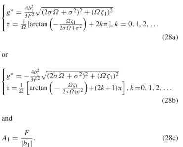
In this section, the effect of feedback gain on the amplitude-delay response curve of the main system is investigated. Figure 3 shows the variation of amplitude of periodic motions with time delay obtained by the integral equa-tion method for six different positive feedback gains, i.e. g∗ ∈ {0.01, 0.1, 0.133, 0.15, 0.2,0.5} while Fig. 4 shows that for the negative feedback gains, i.e. g∗ ∈ {−0.01,−0.1,−0.133,−0.15,−0.2,−0.5}. The amplitude of the main system depends on the feedback gain g∗ and the time delayτ. It is obvious to see that the effect of time
0 2 4 6 8 10 12 0.00 0.05 0.10 0.15 A2 0 2 4 6 8 10 12 0.4 0.6 0.8 1.0 A2 τ τ (a) (b)
Fig. 3 Amplitude-delay response curves of the main system with dif-ferent positive feedback coefficientsg∗.a Pointsstand for unstable solutions,solid linefor stable solutions,blueforg∗ =0.01,red for
g∗ = 0.1,orangeforg∗ =0.133,blackforg∗ = 0.15,purplefor
g∗=0.2,(b)g∗=0.5.(Color figure online)
delay is periodic with periodic 2π/Ω. When|g∗| =0.01, we notice that the amplitude-delay response curves are always stable. However, the efficiency ofτ to suppress the vibra-tion of the main system is inconspicuous. As|g∗|increases, the peak amplitude of the main system increases gradually. The minimum amplitude of the main system decreases first as|g∗|increases from 0.01 to 0.133, and then increases as |g∗|increases further from 0.133 to 0.2. In this process, the stable region of the amplitude-delay curves shrinks. When 0.01 ≤ |g∗| ≤ 0.2, there always exists a tunable range of τ to suppress the vibration. However, the effect of vibra-tion suppression becomes inconspicuous when|g∗| >0.2. Wheng∗=0.2, the periodic solution on the amplitude-delay curve corresponding toτ = 7.85 is unstable and the opti-mal valueτ for vibration suppression is 7. Similarly when g∗ = −0.2, the periodic solution corresponding toτ =11 is also unstable and the optimal value ofτ becomes 10.6. Therefore, the efficiency for vibration suppression becomes slight when|g∗| =0.2. Wheng∗=0.5, vibration reduction is impossible as the amplitude (stable) with time delay is not less than that without. Wheng∗= −0.5, the effect of vibra-tion reducvibra-tion is very slight. Wheng∗≥0.55 org∗≤ −2.1,
0 2 4 6 8 10 12 0.00 0.05 0.10 0.15 τ A2 0 2 4 6 8 10 12 0.4 0.6 0.8 1.0 τ A2 (a) (b)
Fig. 4 Amplitude-delay response curves of the main system with dif-ferent negative feedback coefficientsg∗.aPointsstand for unstable solutions,solid linefor stable solutions,blueforg∗= −0.01,redfor
g∗= −0.1,orangeforg∗= −0.133,blackforg∗= −0.15purplefor
g∗= −0.2,(b)g∗= −0.5.(Color figure online)
the amplitude-delay response becomes fully unstable. For the positive delayed feedback control, it follows from Eqs. (28a) and (28b) that the minimum amplitudes occur when τ =1.57 andτ =7.85. However, the amplitude curves are unstable atτ =1.57. For the negative delayed feedback, the minimum amplitudes occur whenτ = 4.71 and τ = 11. Similarly, the periodic solutions are unstable atτ =4.71.
First, we make a comparison of the analytical results obtained by the integral equation method and the numeri-cal simulations wheng∗ = 0.11 andg∗ = −0.11 in Fig. 5a, b, respectively. It is observed that the analytical results are in good agreement with the numerical simulations, which confirms that the above analysis is valid.
Figure6 shows that the maximum percentage of vibra-tion reducvibra-tion of the main system wheng∗vary from−0.24 to 0.28 with an appropriate time delay. The solid blue line denotes the analytical results and the symbol “+” denotes the numerical results. From this figure, we observe that the amplitude of the main system with time delay can be sup-pressed at different levels. Forg∗varying from 0 to 0.153, the time delay should be fixed at the value of 7.85. Forg∗
0 2 4 6 8 10 12 0.00 0.02 0.04 0.06 0.08 0.10 0.12 0.14 τ A2 0 2 4 6 8 10 12 0.00 0.05 0.10 0.15 τ A2 (a) (b)
Fig. 5 Comparison of amplitude-delay response curves between numerical solutions and analytical solutions obtained by the integral equation method.ag∗=0.11,bg∗= −0.11.Pointsstand for unstable solutions,solid linefor stable solutions and “+” for numerical simula-tion 0.2 0.1 0.0 0.1 0.2 0 20 40 60 80 100 g The of vibration red u ction
Fig. 6 The maximum percentage of the vibration reduction of the main system wheng∗varies from−0.24 to 0.28 with an appropriate time delay. Thesolid linedenotes the analytical results and the “+” denotes the numerical simulation
varying from−0.18 to 0, the time delay should be fixed at τ = 11. For other range ofg∗, the periodic solutions cor-responding toτ = 7.85 andτ = 11 become unstable and the time delay should be chosen near toτ =7.85,τ =1.57
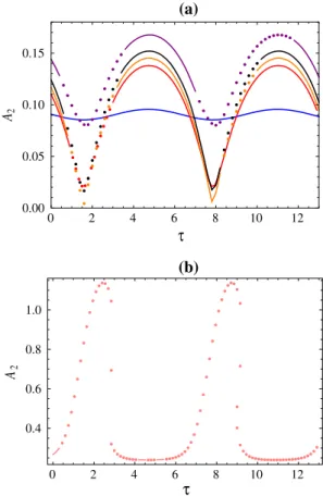
Fig. 7 Time history of the main system forag∗=0.133, τ=0,
bg∗=0.133, τ=7.85
Fig. 8 Time history of the main system for
ag∗= −0.133, τ=0,
bg∗= −0.133, τ=11
(for the positive feedback control) andτ = 11,τ = 4.71 (for the negative feedback control). Forg∗∈ [0.154,0.202], the time delay should be chosen nearτ = 7.85 while for g∗ ∈ [0.203,0.28], it should be chosen nearτ =1.57. For g∗∈ [−0.24,−0.181], the time delay should be chosen near τ =11. From Fig.6, the vibration can be reduced by nearly 100 % wheng∗ =0.133, τ =7.85 andg∗= −0.133, τ = 11. Figure7a, b show the time history of the main system forτ =0 andτ =7.85, respectively wheng∗=0.133. It is seen that the amplitude of the main system can be reduced by 98.53 % from its value without time delay. Forg∗= −0.133, the efficiency of vibration suppression by time delay amounts to 97.83 % as shown in Fig.8. Therefore, the analytical pre-diction is in excellent agreement with the numerical sim-ulations as shown in Figs.7 and 8. Combining Figs.3,4 and6, we observe that the best performance of vibration reduction can be found wheng∗ = 0.133, τ = 7.85 and g∗= −0.133, τ =11. This result is in excellent agreement with the analysis in Sect.4.
7 Force-response curves
In Sect.6, we observe that the optimal vibration reduction occurs whenτ =7.85 for positive feedback gain, andτ =11 for negative feedback gain. In this section, the time delay τ =7.85 orτ =11 is kept fixed.
The effect of varying the feedback gain on the force-response curves of the main system and controller is shown
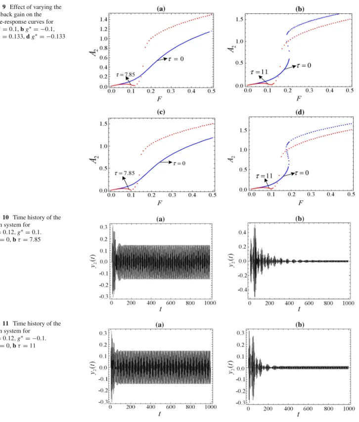
in Fig. 9. Here, four different feedback gains, i.e. g∗ = ±0.1, g∗ = ±0.133 are considered. From Fig. 9, a tun-able range of F to suppress the vibration is obtained when the force amplitude is located in[0.05,0.12].The best vibra-tion suppression points can be obtained whenF =0.12 for g∗ = ±0.1, and F =0.1 forg∗ = ±0.13. Figures10and 11show the time responses of the main system without time delay and with time delay. It can be seen that the amplitude of the main system with appropriate time delay can be reduced by 91 % from its value without time delays when|g∗| =0.1. Figure9also shows that the stability zone decreases under the time-delayed feedback. The parameterFshould be cho-sen in the region [0.05,0.12]. In the region [0.19,0.205] on Fig.9b, varyingF for the force-response curve withτ =0 leads to the jump phenomenon, which results in the coexis-tence of two stable solutions and one unstable solution. The jump phenomenon also occurs in the region [0.176,0.188] in Fig.9d forg∗ = −0.13 whenτ =0, such phenomenon is confirmed from the coexistence of stable solutions obtained in these regions as shown in Figs.12and13.
8 Frequency-response curves
In this section, we investigate the influence of the feedback gain and time delay on the frequency-response curves of the main system. In fact, the stability of the motion, the bifur-cation points and the position for the minimum amplitude depend on time delay.
Fig. 9 Effect of varying the feedback gain on the force-response curves for
ag∗=0.1,bg∗= −0.1,
cg∗=0.133,dg∗= −0.133
Fig. 10 Time history of the main system for
F=0.12,g∗=0.1.
aτ=0,bτ=7.85
Fig. 11 Time history of the main system for
F=0.12,g∗= −0.1.
aτ=0,bτ=11
Figure 14a shows a comparison of frequency-response curve of the main system forτ = 0 andτ = 7.85 when g∗=0.13. We observe that the frequency-response curve is always stable in the frequency interval [−0.5,0.5] forτ =0. The minimum steady-state amplitude of the main system occurs for the detuning parameterσ2=0.03. Forτ =7.85,
the minimum amplitude of the main system occurs when σ2 = 0. The frequency-response curve is stable for large
negative value of σ2. At σ2 = −0.18, the curve becomes
unstable due to a saddle-node bifurcation. However, the solu-tion becomes stable again whenσ2 = −0.02. Forσ2
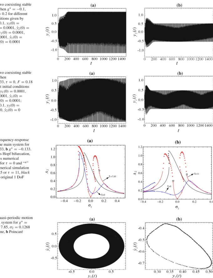
Fig. 12 Two coexisting stable solutions wheng∗= −0.1, τ=0,F=0.2 for different initial conditions given by
ay1(0)=0.1,y2(0)=
0.2,y˙1(0)=0.0001,y˙2(0)=
0.0001;by1(0)=0.0001, y2(0)=0.0001,y˙1(0)=
0.0001,y˙2(0)=0.0001
Fig. 13 Two coexisting stable solutions when
g∗= −0.133, τ=0,F=0.18 for different initial conditions given byay1(0)=0.0001, y2(0)=0.0001,y˙1(0)= 0.0001,y˙2(0)=0.0001; by1(0)=0.1,y2(0)= 1,y˙1(0)=0,y˙2(0)=0 Fig. 14 Frequency-response curves of the main system for
ag∗=0.133,bg∗= −0.133.
Boxdenotes Hopf bifurcation, “+” denotes numerical simulation forτ=0 and “*” denotes numerical simulation forτ=7.85 orτ=11,black
linefor the original 1 DoF system τ=7.85 τ=0 0.4 0.2 0.0 0.2 0.4 0.0 0.2 0.4 0.6 0.8 1.0 1.2 σ2 σ 2 A2 A2 τ=11 =0 τ 0.4 0.2 0.0 0.2 0.4 0.0 0.2 0.4 0.6 0.8 1.0 1.2 (a) (b)
Fig. 15 Quasi-periodic motion of the main system forg∗=
0.133, τ=7.85, σ2=0.1268 aphase plane,bPoincaré section
the smallest solution is stable. On the other hand, whenσ2
decreases from 0.5, the frequency-response curve is initially stable and becomes unstable atσ2=0.1271 due to a Hopf
bifurcation. Asσ2decreases further, a quasi-periodic solution
comes into existence atσ2=0.1269 due to a secondary Hopf
Bifurcation. As shown in Fig.15, a quasi-periodic solution is obtained by numerical simulation atσ2=0.1268.
Figure 14b shows a comparison of frequency-response curve of the main system for τ = 0 and τ = 11 when g∗ = −0.133. Forτ = 0, a jump phenomenon occurs in
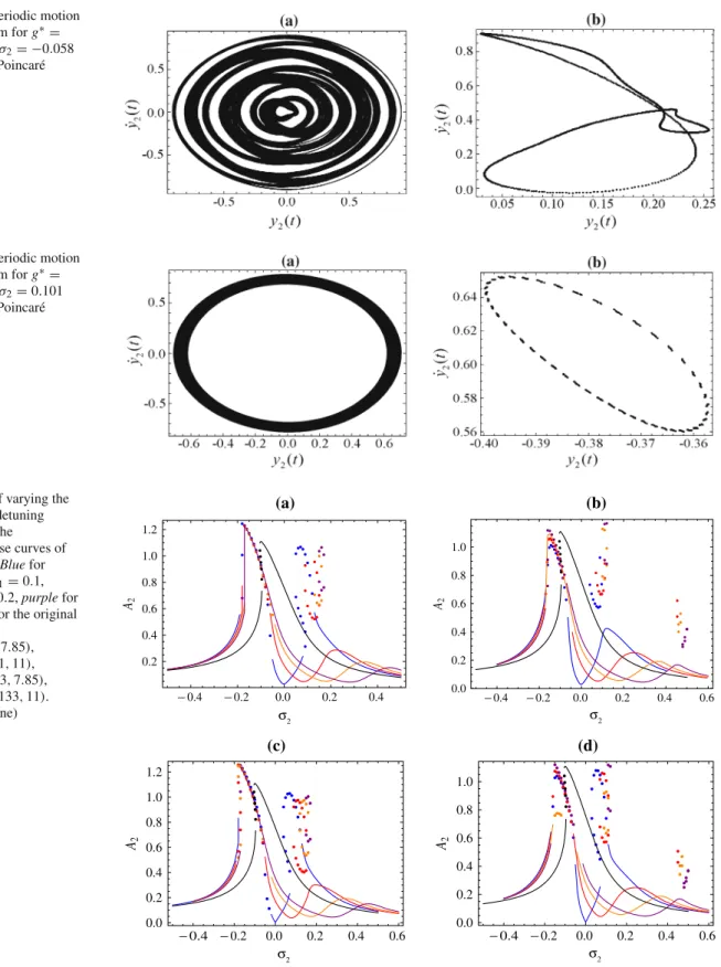
Fig. 16 Quasi-periodic motion of the main system forg∗=
−0.133, τ=11, σ2= −0.058 aphase plane,bPoincaré section
Fig. 17 Quasi-periodic motion of the main system forg∗=
−0.133, τ=11, σ2=0.101 aphase plane,bPoincaré section
Fig. 18 Effect of varying the positive internal detuning parameterσ1on the
frequency-response curves of the main system.Bluefor σ1=0,redforσ1=0.1, orangeforσ1=0.2,purplefor
σ1=0.3,blackfor the original
1 DoF system.
a(g∗, τ)=(0.1,7.85),
b(g∗, τ)=(−0.1,11),
c(g∗, τ)=(0.133,7.85),
d(g∗, τ)=(−0.133,11). (Color figure online)
0.4 0.2 0.0 0.2 0.4 0.2 0.4 0.6 0.8 1.0 1.2 A2 0.4 0.2 0.0 0.2 0.4 0.6 0.0 0.2 0.4 0.6 0.8 1.0 A2 0.4 0.2 0.0 0.2 0.4 0.6 0.0 0.2 0.4 0.6 0.8 1.0 1.2 A2 0.4 0.2 0.0 0.2 0.4 0.6 0.0 0.2 0.4 0.6 0.8 1.0 A2 σ2 σ2 σ2 σ2 (a) (b) (c) (d)
the region [−0.4,−0.25], which implies the coexistence of two unstable solutions and one stable solution. The minimum amplitude of the main system occurs whenσ2= −0.03. For
τ =11, the jump phenomenon disappears. The frequency-response curve has three stable segments:σ2<−0.17, σ2∈
[−0.056,0.08]andσ2 >0.101. Hopf bifurcation occurs at
σ2= −0.056 andσ2=0.101 while saddle-node bifurcation
atσ2= −0.17 andσ2=0.08. Three solutions coexist in the
region [0.028,0.08], and the lowest branch is stable. Quasi-periodic solutions are observed in the unstable segments.
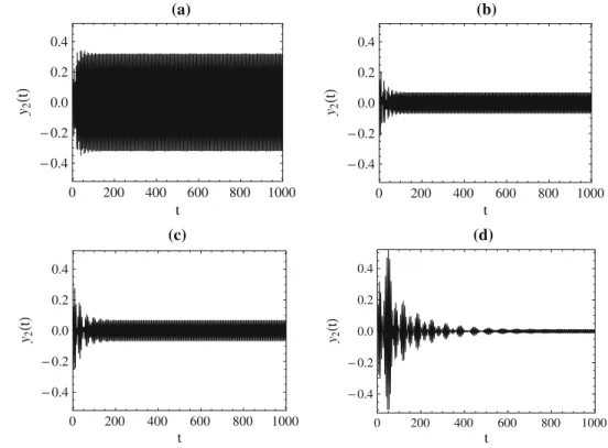
Fig. 19 Time history of the main system for
aσ1=0.1, σ2=0.25, bσ1=0.25, σ2=0.25, cσ1=0.1, σ2=0.1, dσ1=σ2=0 0 200 400 600 800 1000 0.4 0.2 0.0 0.2 0.4 t y2 t 0 200 400 600 800 1000 0.4 0.2 0.0 0.2 0.4 t y2 t 0 200 400 600 800 1000 0.4 0.2 0.0 0.2 0.4 t y2 t 0 200 400 600 800 1000 0.4 0.2 0.0 0.2 0.4 t y2 t (a) (b) (c) (d)
Figures16and17show such solutions atσ2= −0.058 and
σ2=0.101, respectively.
Based on the frequency-response curves in Fig.14, we can conclude that time delays can change the position where the minimum amplitude of the main system occurs. It is found that the frequency-response curves forτ =0 are lower than that forτ =0 nearσ2=0, which means that there exists a
tunable range ofσ2for the vibration suppression nearσ2=0.
The time delay may result in the disappearance of the jump phenomenon and the occurrence of Hopf Bifurcations.
Figure18shows the effect of varying the positive inter-nal detuning parameterσ1on the frequency-response curves
for the four cases(g∗, τ)∈ {(0.1,7.85), (−0.1,11), (0.133, 7.85), (−0.133,11)}forσ1∈ {0,0.1,0.2,0.3}. For all these
cases, we observe that the minimum amplitude of the main system occurs nearσ1 = σ2. This result can be explained
from the optimal solution obtained from (29). Recall that we choose ω1 = ω2 = Ω = 1 for our investigation. It
fol-lows from (10) and (21) thatσ =σ1−σ2=0. In Fig.18,
since the control parameters (g∗, τ) satisfy (29), the min-imum amplitude of the main system occurs whenσ = 0, i.e. σ1 = σ2. Therefore, it is important to tune the
nat-ural frequency ω1 of the controller to near the excitation
frequencyΩ. This results are in excellent agreement with previous work [20]. Figure19shows the time history of the main system for the four cases (a)σ1 = 0.1, σ2 = 0.25,
(b) σ1 = 0.25, σ2 = 0.25, (c) σ1 = 0.1, σ2 = 0.1, (d)
σ1=0, σ2=0 wheng∗=0.1, τ =7.85. It is clear that the
amplitude of the main system can be much reduced by set-tingσ1=σ2. Moreover, the best performance of the vibration
reduction occurs whenσ1=σ2=0 forg∗=0.1, τ =7.85.
The numerical simulations in Fig.19are in good agreement with the above analysis from Fig.18.
9 Conclusions
A nonlinear time delayed feedback controller is designed to reduce the vibration of the main system in a two-degree-of-freedom nonlinear system with external excitation. The integral equation method is applied to derive four amplitude equations of the system when the primary resonance and 1:1 internal resonance occur simultaneously. Then, the sta-bility of the system is analyzed using the Floquet theory to assess the performance of the feedback gain and time delay on vibration suppression.
Although the amplitude equations (17)–(20) look very complicated, analytical expression of the optimal feedback gaing∗and time delayτcan be obtained such that the ampli-tude of the main system vanishes. Two values of optimal feedback gain are found, which are in opposite sign of the same magnitude(±g∗). For the system parameters we have considered, excellent vibration suppression can be achieved. Applying the positive optimal feedback gain(g∗=0.133), the amplitude of the main system can be reduced by 98.53 % in comparison with the amplitude without time delay. On the other hand, applying the negative optimal feedback gain (g∗ = −0.133), the amplitude reduction is 97.83 %.
percentage of amplitude reduction decreases rapidly. There-fore, finding the optimal feedback gain and time delay is crucial in the vibration control of this system.
When the time delay is fixed at the optimal value obtained from the integral equation method, it is important to tune the natural frequencyω1of the controller to near the
exter-nal excitation frequencyΩfor effective vibration reduction. Ifω1 deviates much fromΩ, Hopf and even second Hopf
bifurcations may occur which ruins the purpose of vibration control.
Acknowledgments This work is supported by the Hong Kong Research Grant Council under CERG Grant (CityU 1005/07E), the State Key Program of National Natural Science Foundation of China under Grant No. 11032009 and National Natural Science Foundation of China under Grant No. 11272236.
References
1. Diekmann O, VanGils SA, Verduyn Lunel SM, Walther HO (1995) Delay equations, functional, complex, and nonlinear analysis. Springer-Verlag, New York
2. Belair J, Campbell SA (1994) Stability and bifurcation of equi-libria in a multi-delayed differential equation. SIAM J Appl Math 54:1402–1424
3. Stépán G, Haller G (1995) Quasiperiodic oscillations in robot dynamics. Nonlinear Dyn 8:513–528
4. Reddy DVR, Sen A, Johnston GL (1998) Time delay induced death in coupled limit cycle oscillators. Phys Rev Lett 80:5109–5112 5. Wirkus S, Rand R (2002) The dynamics of two coupled van der
Pol oscillators with delay coupling. Nonlinear Dyn 30:205–221 6. Xu J, Chung KW (2003) Effects of time delayed position feedback
on a van der Pol-Duffing oscillators. Physica D 180:17–39 7. Hu H, Dowell EH, Virgin LN (1998) Resonances of a harmonically
forced Duffing oscillator with time delay state feedback. Nonlinear Dyn 15:311–327
8. Maccari A (2001) The response of a parametrically excited van der Pol oscillator to a time delay state feedback. Nonlinear Dyn 26:105–119
9. Siewe M, Tchawoua C, Rajasekar S (2012) Parametric resonance in the Rayleigh–Duffing oscillator with time-delayed feedback. Com-mun Nonlinear Sci Numer Simulat 12:4485–4493
10. El-Gohary HA, El-Ganaini WAA (2012) Vibration suppression of a dynamical system to multi-parametric excitations via time-delay absorber. Appl Math Modell 36:35–45
11. Leung AYT, Guo ZJ, Myers A (2012) Steady state bifurcation of a periodically excited system under delayed feedback controls. Com-mun Nonlinear Sci Numer Simulat 17:5256–5272
12. Zhao YY, Xu J (2007) Effects of delayed feedback control on non-linear vibration absorber system. J Sound Vib 308:212–230 13. Zhao YY, Xu J (2008) Mechanism analysis of delayed nonlinear
vibration absorber. Chin J Theor Appl Mech 40:98–106
14. Schmidt G, Tondl A (1986) Nonlinear vibrations. Cambridge Uni-versity Press, Cambridge
15. Chen YL, Xu J (2013) Applications of the integral equation method to delay differential equations. Nonlinear Dyn 73:2241–2260 16. Li XY, Zhang LJ, Zhang HB, Li XL (2011) Delayed feedback
con-trol on a class of generalized gyroscope systems under parametric excitation. Procedia Eng 15:1120–1126
17. Li XY, Ji JC, Hansen CH, Tan CX (2006) The response of a Duffing-van der Pol oscillator under delayed feedback control. J Sound Vib 291:644–655
18. Nayfeh AH, Chin CM, Pratt J (1997) Perturbation methods in non-linear dynamics-applications to machining dynamics. J Manuf Sci Eng 119:485–493
19. Daqaq MF, Alhazza KA, Arafat HN (2008) Nonlinear vibrations of cantilever beams with feedback delays. Int J Non-linear Mech 43:962–978
20. El-Ganaini WA, Saeed NA, Eissa M (2013) Positive position feed-back (PPF) controller for supperssion of nonlinear system vibra-tion. Nonlinear Dyn 72:517–537