c
Sharif University of Technology, February 2009
Application of a Maintenance Management
Model for Iranian Railways Based on the Markov
Chain and Probabilistic Dynamic Programming
Y. Shafahi
1;and R. Hakhamaneshi
1Abstract. Railway managers have a strong economic incentive to minimize track maintenance costs, while maintaining safety standards and providing adequate service levels to train operators. The objective of this study is to apply a procedure for making optimal maintenance decisions in Iranian Railways. This study consists of two parts. First, a cumulative damage model, based on a Markov process, is applied to model the deterioration of the track. For this reason, tracks are categorized into six classes, so that those tracks with similar trac loads and geographical location are collected into one class. The track survey data from 215 blocks (4,228 km) of the ten divisions of the Iranian Railway system, during 2002-2004, is used to identify the transition matrix. Secondly, probabilistic dynamic programming is used to nd the optimal repair for each possible track state in the planning horizon. This approach allows an optimal maintenance decision to be determined for the track at any point in time within the planning horizon. Keywords: Maintenance management; Railways; Markov chain; Dynamic programming.
INTRODUCTION
The railway is a branch of the transportation system that is very expensive to construct, but which has a long life and low operating costs. Therefore, the asset value is very high, which also leads to the possibility that maintenance might prove expensive. Like other infrastructures with high investment costs in the construction phase, maintenance plays a crucial role in its long-term cost eectiveness.
Maintenance planning for deteriorating facilities seems to be hard because of their random aspects. The process of the track deterioration is aected by weather and trac loads randomly. Although such uncertainties exist, railway managers should be asking when the track will need to be repaired and which types of repair will be the best choice. In this paper, an eort will be made to apply a model in answer to these questions for tracks in the Iranian Railway system.
The condition or \state" of a track dictates the
1. Department of Civil Engineering, Sharif University of Tech-nology, P.O. Box 11155-8639, Tehran, Iran.
*. Corresponding author. E-mail: [email protected] Received 14 April 2007; accepted 1 July 2007
cost of maintenance directly. Trac loads, weather, the geometrics of the track and construction materials are the most important factors that aect the track de-terioration process. However, it is observed that, even when these factors are similar, the track deterioration rate may be unexpectedly dierent. Thus, a model that can handle this problem in such dimensions is necessary for any railway system.
Several approaches and methods have been pro-posed and, based on these, a considerable number of maintenance planning tools have been developed for various railway systems in North America and Europe. A nonlinear regression model, based on a product of the power functions, has been proposed by the Oce for Research and Experiments (ORE) of the International Union of Railways [1] to predict track deterioration. Operation research techniques are commonly used to optimize track maintenance activity. Such approaches have been described by Esveld [2] and Zarembski [3]. Zhang [4] has proposed an Integrated Track Degradation Model (ITDM). ITDM simulates track degradation, based on the interaction between dierent track components under varying trac. It also considers several mechanistic characteristics, including train speed and axle load. Based on the ITDM,
Simson et al. [5] have developed a Track Maintenance Planning Model (TMPM), which aims to deal with track maintenance planning in the medium to long term. TMPM outputs the net present value of the nancial benets of undertaking a given maintenance strategy compared with a base-case maintenance sce-nario. The Total Right-of-way Analysis and Costing System (TRACS) has been described by Martland et al. [6]. It is a system (software) developed by the Association of American Railroads (AAR) and the Massachusetts Institute of Technology (MIT) in the USA. It is a computer-based tool developed to assist rail management to address change in the infrastruc-ture. By combining engineering-based deterioration models with life-cycle costing techniques, the model estimates track maintenance and renewal costs as a function of route geometry, track components and track conditions, as well as trac mix and volume. TRACS has been used by North American railroads as a tool for technology assessment costing, in support of actions such as pricing, budgeting and line con-solidation. Both the ITDM and the TRACS models are based on an incremental approach, where each event, such as rail grinding, relining and track renewal, can be included. In recent years, the application of soft computing techniques has paid attention to predicting future track conditions and Shafahi and Rasooli [7] have considered neuro-networks to pre-dict such conditions. A neuro-fuzzy decision support system for rail track maintenance planning has been described by Dell'Orco et al. [8]. During the 1990s, the International Railway Union (UIC), in conjunction with the European Rail Research Institute (ERRI), developed an expert system for track maintenance and renewal (ECOTRACK). This model builds on the fact that rules can be specied for certain maintenance ac-tivities under certain conditions. A historical database, containing infrastructure information on components and current conditions, is also a prerequisite to using this model. ECOTRACK solves the planning problem, given the rules specied, and points out the activities needed at each section at certain times. Recent work on ECOTRACK at ERRI [9] has developed the model further, in order to improve its functional-ity.
Determining optimal maintenance during a plan-ning horizon, while minimizing maintenance costs and satisfying certain constraints in a railway system, is the objective of this study. To reach this objective, a method similar to Carnahan et al.'s procedure [10] for Pavement Management System is chosen and applied to Iranian Railway data. This approach consists of two parts. First, a Markov model for track deterio-ration is introduced. Second, a probabilistic dynamic programming is used to nd the optimal repair ac-tions.
The rest of the paper is organized as follows. First, the prediction of track conditions by using the Markov model is discussed. Then, the results of using Markov and ORE models are compared. Following that, the dynamic programming procedure that is used to solve maintenance scheduling problems is described. And, nally, the main conclusions are summarized. PREDICTION OF TRACK CONDITION USING MARKOV MODEL
Track condition is one of the most important param-eters aecting track maintenance management. In order to obtain a good track maintenance management system, it is necessary to predict track conditions through time. As mentioned earlier in this paper, trac loads, weather, geometrics of the tracks and construction materials are the most important factors to aect the track deterioration process. However, it is observed that, even when these factors are similar, the track deterioration rate may be unexpectedly dierent. Because of this random behavior, using a probabilistic model seems to be a good procedure for predicting track conditions. The Markov process has the char-acteristics to explain the random behavior of a track clearly during its deterioration.
To describe the condition of the track, several indexes and criteria have been dened and used in dierent railway systems around the world. Commonly, the Track Quality Index (TQI) is used to dene the track quality. TQI is normally determined by Track Geometry Parameters (TGP). The term `track deterioration' is used to describe any changes in track geometry. Track deteriorations are classied as: un-evenness, twist, alignment and gauge. TQI is a function of these four parameters.
In this study, the track state will be dened in terms of the Combined Track Record index (CTR index) rating, which can vary from 0 to 100, where 100 denotes the best possible track condition and the states are dened as ve intervals of the CTR index (Table 1). It is supposed that the track began its life, at some time in the past, in near-perfect condition. It was then subject to a sequence of duty cycles that caused its condition to deteriorate. The duty cycle for the track in this study will be assumed to consist of one year's weather and trac load. These discrete state and discrete time unit denitions let one express the deterioration process as a Markov chain.
To have better models, in this study, the tracks are categorized so that those with similar trac load and geographical location are collected into one class. A network of tracks, based on the topography, was di-vided into three groups of plain, hilly and mountainous areas, and based on trac load, was divided into two
Table 1. Track state classication by CTR index.
CTR Index 0-50 50-60 60-70 70-80 80-100 Track Quality Failed Medium Good Very good Excellent Track State 1 2 3 4 5
groups of light and heavy trac. There are, thus, six track classes (Table 2).
The basic assumption for a Markov process is that the probabilities of going from one state to another depend only on the current state, and not on the manner in which the current state is reached. This property is often called the `memoryless' property of the process. In this case, this is a reasonable assumption. Let:
pij= Probability that a track will be in state j in
the next year when it is currently in state i, P = [pij] is the transition matrix, which shows
the probabilities of various state transitions. The authors' data shows that the track condition will almost never decrease more than 10 CTR index in a year. Thus, one can assume that, during each duty cycle (a year), a track will either stay in its current state or jump to the next lowest state. Thus, the nonzero elements of the matrix, `P ', consist of diagonal and adjacent lower diagonal elements. In other words: pii= pi= The probability that a track will stay in its
current state, i, in the next duty cycle,
pi(i 1)=1 pi=qi= The probability that a track will
be in state i 1 when it is currently in state i, pij = 0 for all j 6= i, i 1 and i 1 > 0: (1)
Then, the transition matrix becomes:
P = 2 6 6 6 6 4
1 0 0 0 0
q2 p2 0 0 0
0 q3 p3 0 0
0 0 q4 p4 0
0 0 0 q5 p5
3 7 7 7 7
5: (2)
The state of the track at any time, n, n = 1; 2; can be expressed in a probabilistic manner as a (1 5) row
Table 2. Iranian Railways' classication by topography and trac conditions (K).
Trac Topography Condition Condition Plain
Areas
Hilly Areas
Mountainous Areas
Light 1 2 3
Heavy 4 5 6
vector p(n):
p(n)=(pfX(n)=1g; pfX(n)=2g; ; pfX(n)=5g); (3) where X(n) is the track state at time n and pfX(n) = jg is the probability that a track is in state j at time n. Obviously, the elements of the vector, p(n), must sum to 1.0.
The initial state of the track is given by p(0). For example, if one supposes that the track was in excellent condition when it was new, then:
p(0) = (0; 0; 0; 0; 1): (4)
Other initial state vectors may be dened to reect the uncertainty in the initial condition of the track.
It can be shown [11] that the state vector at some future time may be calculated from the transition matrix and the initial state vector, as follows:
p(1) = p(0)P
p(2) = p(1)P = p(0)P2
p(n) = p(0)Pn:
(5)
Or, more generally,
p(m + n) = p(m)Pn: (6)
The collected data for the state of the tracks during their lives may be used to estimate the transition matrix, P . To accomplish this task, a data base containing these data is built, as well as several other operational characteristics of the track.
Data Bank
The data for this empirical application was collected from the Iranian Railways network and incorporated four types of survey: Topography, annual trac and axle load, date of construction or reconstruction and the track condition of the block in each year. In this study, the block, which is the distance between two consecutive stations in the network of tracks, is the smallest maintenance unit, similar to those used by Iranian Railways.
Nowadays, the condition of railways is monitored by special diagnostic trains. MATISA, the diagnostic train for Iranian Railways, measures the geometric parameters of the railway track, such as: Alignment, gauge, cross-level and prole, in order to allow one to nally compute the average CTR index for the blocks.
The Iranian Railway network consists of 7,203 km of track (in 2004). Topography, annual trac load, axle load and the latest date of construction or reconstruction for 215 blocks (4,228 km) were collected from the Iranian Railway system and the average CTR indexes of these blocks for three years (2002-2004) were computed. These data were col-lected from dierent divisions of the Iranian Rail-ways, including Shomaleshargh, Khorasan, Shoma-legharb, Azarbayegan, Gonoob, Lorestan, Shomal, Arak, Gonoobeshargh and Hormozgan. On the basis of this data, 60% (122 blocks, 2,544 km) are in plain areas, 19% of these tracks (44 blocks, 797 km) are in hilly areas, and 21% (49 blocks, 887 km) in mountainous areas. 70% of these tracks have been designed for 20-tonne axle loads and the rest for 25-20-tonne axle loads. Furthermore, 36% of them (72 blocks, 1,525 km) have heavy trac passing over them.
Estimation of the Transition Matrix
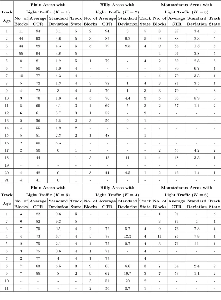
It is necessary to transform the track survey data into the CTR index versus age, in order to use the data for estimating the transition matrix. To do so, the age of the track is dened as the dierence between the current date (date of geometric parameter recording) and the latest date of reconstruction or construction. The CTR index, geographical location, annual trac load and the latest date of reconstruction or construction of the blocks must be specied to identify the transition matrix, P . The CTR index versus the age data was specied by computing the average CTR index of the blocks that are of the same age in each class. Thus, the track state was specied on the basis of the observed condition of the track. Table 3 summarizes the CTR index versus index versus the age data. On the basis of Table 3, there are some blocks that are more than 20 years old in light trac blocks. This means that there are some blocks that have not been repaired for 20 years in the light trac tracks in the Iranian Railways, but, in heavy trac tracks, there are no blocks that are more than 9 years old.
The sum of the squared dierences between the expected state predicted from the Markov process (Equations 5) and the observed track condition at each age for which data were available is used as the objec-tive function to estimate the transition matrix. Mini-mizing this objective function produces the elements of
the transition matrix. The Quasi-Newton method [12] was used to minimize this objective function. Using an initial guess for the transition matrix elements and an excellent condition for the initial state vector, the minimization algorithm obtained the transition matrices. An independent transition matrix (Table 4) was computed for each track class. The descending process of the probability of staying in the current state in all six classes represents the fact that the track deterioration rate accelerates when the tracks are badly deteriorated. It means that, in badly deteriorated states, the inclination to jump to a lower state increases (note the low dierences between the respective gures in columns p5 and p4 and the signicant dierences
between those in columns p3 and p2 in Table 4).
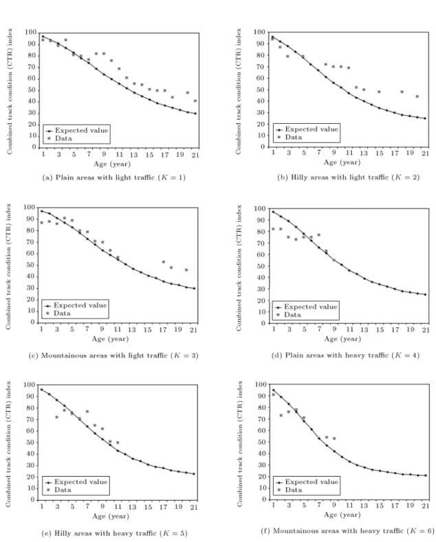
Furthermore, Table 4 also shows that tracks with light trac have little dierence in the deterioration rates across track classes. Moreover, for heavy trac, tracks in mountainous areas have rates of deterioration faster than those in plain or hilly areas. Figure 1 shows the observed data and the expected value of the transition matrix that minimized the objective function for the six classes of track.
A COMPARISON OF THE MARKOV MODEL WITH THE ORE MODEL
The ORE of the International Union of Railways proposed a simple model of track deterioration in the more general form of a product of the power functions in 1988. In this paper, the ORE model is rebuilt using the existing data bank and the results are compared with the proposed Markov model. Equation 7 shows the rebuilt ORE model:
E = 36:57 T 0:0418 P0:2955; (7)
where:
E a track degradation index (in this paper, CTR index);
T total accumulated tonnage since the track was new (million tones);
P design axle load (tone).
The number of observations is 523 and all estimated parameters are within the 95% condence interval.
For the comparison of two models, linear regres-sion between the observation and estimation of each model is used. Table 5 shows the results. Obviously, when the regression coecient, \a", is close to 1.0 and signicantly dierent from 0, and the coecient, \b", is close to 0.0 and insignicant, the model is a good predictor of the actual observations. The R2 values in
Table 5 also show that the Markov model predicts track deterioration better than the ORE model.
Table 3. Summary of CTR index versus age data for dierent classes of tracks (K = 1 to 6).
Plain Areas with Hilly Areas with Mountainous Areas with Track Light Trac (K = 1) Light Trac (K = 2) Light Trac (K = 3)
Age No. of Blocks
Average CTR
Standard Deviation
Track State
No. of Blocks
Average CTR
Standard Deviation
Track State
No. of Blocks
Average CTR
Standard Deviation
Track State 1 11 94 3.1 5 2 94 0 5 8 87 3.4 5 2 44 93 4.6 5 3 87 6.2 5 9 88 2.3 5 3 44 89 4.3 5 5 79 8.5 4 9 86 1.3 5
4 55 94 4.6 5 - - - - 4 91 3.8 5
5 8 81 1.2 5 1 79 - 4 2 89 2.8 5
6 7 80 1.0 4 - - - - 5 80 6.7 4
7 10 77 4.3 4 - - - - 4 79 3.3 4
8 5 72 1.3 4 3 72 1 4 3 71 3.5 4
9 4 72 3 4 4 70 1 3 3 70 1 3
10 3 76 1.0 4 5 70 4.4 3 5 63 8.9 3 11 5 69 4.1 3 4 69 5 3 2 57 1.4 2
12 6 61 3.7 3 1 52 - 2 - - -
-13 5 56 1.8 2 3 50 0 1 - - -
-14 4 55 1.9 2 - - -
-15 5 51 2.3 2 1 48 - 1 - - -
-16 2 50 6.3 1 - - -
-17 2 50 0 1 - - - - 2 53 4.2 2
18 1 44 - 1 3 48 11 1 4 48 3.3 1
19 - - -
-20 4 48 0 1 3 44 4.5 1 2 46 1.4 1
21 4 41 0 1 - - -
-Plain Areas with Hilly Areas with Mountainous Areas with Track Light Trac (K = 5) Light Trac (K = 4) Light Trac (K = 6)
Age No. of Blocks
Average CTR
Standard Deviation
Track State
No. of Blocks
Average CTR
Standard Deviation
Track State
No. of Blocks
Average CTR
Standard Deviation
Track State
1 3 82 0.6 5 - - - - 1 91 - 5
2 6 82 9.2 5 - - - - 3 73 1 4
3 7 75 15 4 2 72 5.7 4 9 76 7.3 4 4 4 73 8.7 4 5 78 12.2 4 11 78 7.8 4 5 2 75 2.1 4 4 75 9.7 4 3 71 11 4
6 3 75 0.6 4 1 71 - 4 - - -
-7 3 77 4 4 1 77 - 4 - - -
-8 7 63 6.5 3 9 65 6.6 3 7 54 2.4 2 9 7 55 8 2 9 62 10.7 3 7 53 1.1 2
10 - - - - 3 51 20 2 - - -
-Table 4. Diagonal elements of transition matrices for the 6 classes of tracks. Track Class (K) Terrain Trac p2 P3 p4 p5
1 Plain Light 0.3957 0.6104 0.7565 0.8641 2 Hilly Light 0.1264 0.6497 0.7365 0.8151 3 Mountainous Light 0.1931 0.5247 0.7310 0.8732 4 Plain Heavy 0.3404 0.5314 0.6753 0.8390 5 Hilly Heavy 0.3296 0.5546 0.7085 0.8067 6 Mountainous Heavy 0.1633 0.4897 0.6593 0.7417
Figure 1. Comparison of expected state from cumulative damage model with track condition data for tracks in the 6 classes under study.
Table 5. Results of Markov and ORE models. Model Observation-Estimation Relation
a (t-stat) b (t-stat) R2
ORE 0.119 (2.986) 72.810 (21.943) 0.119 Markov 0.779 (18.608) 20.008 (6.738) 0.832
NOTE: Observation-estimation relation: y = ax + b (x =observation, y = estimation)
DYNAMIC PROGRAMMING SOLUTION FOR TRACK MAINTENANCE
SCHEDULING
If the track deterioration process is modeled as a Markov process, probabilistic dynamic programming is a convenient method to nd the optimal maintenance decisions. Dynamic programming is a mathematical technique designed to solve decision problems, in which there are a sequence of related decisions to make. The method of solution is to divide the total problem into a number of sub problems, then, working backward from the end of the problem; each problem is solved in turn. Suppose the planning horizon of the study is N years, let:
n year number; n = 1; 2; ; N XK(n) the state of a track of class K in
year n; XK(n) = 1; 2; ; 5
PK the transition matrix for the track
of class K
Rj the repair alternative j = 0; 1; 2,
representing routine maintenance, track improvement and track reconstruction, respectively CK[XK(n); Rj] Cost of implementation alternative
Rj for the track of class K when
the current state of the track is XK(n)
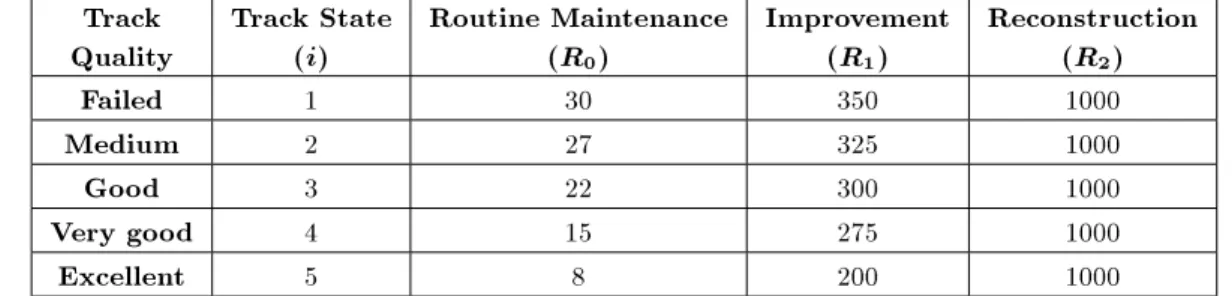
The estimates of the costs used in this study are obtained from the Financial Aairs Oce of Iranian Railways and are given in Table 6 for the year 2004.
It is supposed that the costs of all alternatives are functions of the state of the track, except for recon-struction that is not state dependent. For simplicity, none of the costs are assumed to be dependent on the track classication index, K. Some constraints may be considered in this process. For example, the track condition can be constrained in any year, so that the track state, XK(n), is kept above some minimum
level, Xmin(n), with a specied probability, pmin(n), as
suggested by Carnahan et al. [10]. These constraints may be enforced in any year of the planning horizon or, perhaps only in the last year.
Starting with the optimal decision in the last year of the planning horizon, we work backward on a recursive relationship that nds the decisions in all previous years. The feasibility of the repair alternative is decided in a straightforward manner. Repair alter-natives, R1 and R2, are always feasible, since, when
they are implemented, the track state is upgraded to an excellent condition. But, the feasibility of alternative R0 always must be tested for the following condition:
XK(n) 1X
min(n); or (XK(n)=Xmin(n)=j;
and pK
j pmin(n)): (8)
The optimal repair alternative, R[XK(n)], with
min-imum cost, CK[XK(n)], is chosen among the feasible
alternatives. After an optimal repair is determined for year n, we can nd the optimal decisions for all subsequent stages by developing a recursive rela-tionship. Since a \backwards pass" is being made with the dynamic programming algorithm, these stages correspond to previous years in the planning horizon. Now, as in [10], let:
CK
j;n(i) = The expected cost of stages n; n + 1; ;
N when the state of track is i at the beginning of stage n and repair alternative Rj is chosen for tracks in
class K.
If R0 is infeasible, then C0;nK (i) is set to innity;
Table 6. Costs of repair alternative (in million Rials per kilometer) for various states (i) and repair alternative Rj: CK[i; Rj].
Track Quality
Track State (i)
Routine Maintenance (R0)
Improvement (R1)
Reconstruction (R2)
Failed 1 30 350 1000
Medium 2 27 325 1000
Good 3 22 300 1000
Very good 4 15 275 1000
Excellent 5 8 200 1000
otherwise, the CK
0;n(i) is computed as:
CK
0;n(i) = CK[XK(n) = i; R0]
+ pK
i CK[XK(n + 1) = i]
+ (1 pK
i )CK[XK(n + 1) = i 1];
i = 1; 2; : : : ; 5; n = 1; 2; : : : ; N: (9) C0k can also be computed by:
C0K
n (i) = minRj j>0
fCK[XK(n); R j]
+ pK
5CK[XK(n + 1) = 5]
+ (1 pK
5 )CK[XK(n + 1) = 4]g;
i = 1; 2; ; 5; n = 1; 2; ; N: (10) The optimal repair cost for state XK(n) is computed
as: CK
n (i) = minfC0nK(i); C
0K
n (i)g; (11)
where CK
n (i) is the minimum expected costs over the
remaining planning horizon, when the track is found in state XK(n) = i at the beginning of stage n for tracks
in class K and: CK
N+1= 0; for all i and all K:
Actually, determining the optimal repair alternative in any year, n, requires knowledge of the optimal repair alternative for each state in the following year. By starting in year N of the planning horizon, the optimal repair for years (N 1; N 2; ; 2; 1) can be determined from this recursive approach.
Using the state transition matrices, PK (Table 4),
and the costs for each repair alternative, Rj (Table 6),
one may start the computation process. The feasibility of repair alternatives available for each track state was also modied using expert judgment. For example, for failed track, reconstruction is the only feasible alterna-tive. Improvement is not permitted, since it will not restore the failed track to an excellent condition. The process may then determine those particular actions that are not feasible, rather than having them excluded from the feasible set.
The steps of the algorithm are as follows: Step 1. Let n = N, K = 1 and i = 1 (n = year, K =
track class, and i = track state, indices); Step 2. Check feasibility of repair alternatives
(Equa-tion 8 and expert judgment);
Step 3. Calculate CK
j;n(i) (Equations 9 and 10), for all
j; given i, n and K;
Step 4. Calculate the optimal repair cost for state i, CK
n (i) (Equation 11); given i, n and K;
Step 5. Identify the minimum cost repair alternative, R
n(i); given i, n, K;
Step 6. If i < x, then i + 1 ! i and go to Step 2, otherwise, continue (here, x = maximum track state index = 5);
Step 7. If K < k, then 1 ! i, K + 1 ! K and go to Step 2, otherwise, continue (here, k = maximum track class index = 6);
Step 8. If n > 1, then 1 ! i, 1 ! K, n 1 ! n and go to Step 2, otherwise, stop. Final solution is attained.
A computer program was developed to implement the algorithm. The optimal maintenance program was obtained for a 10-year planning horizon, rst without any constraint and, then, with the single constraint that the track state be at least 3 in year 10, with a probability of 0.95. That is, in this case, for any K, N = 10, pk
min(10) = 0:95 and Xmink (10) = 3.
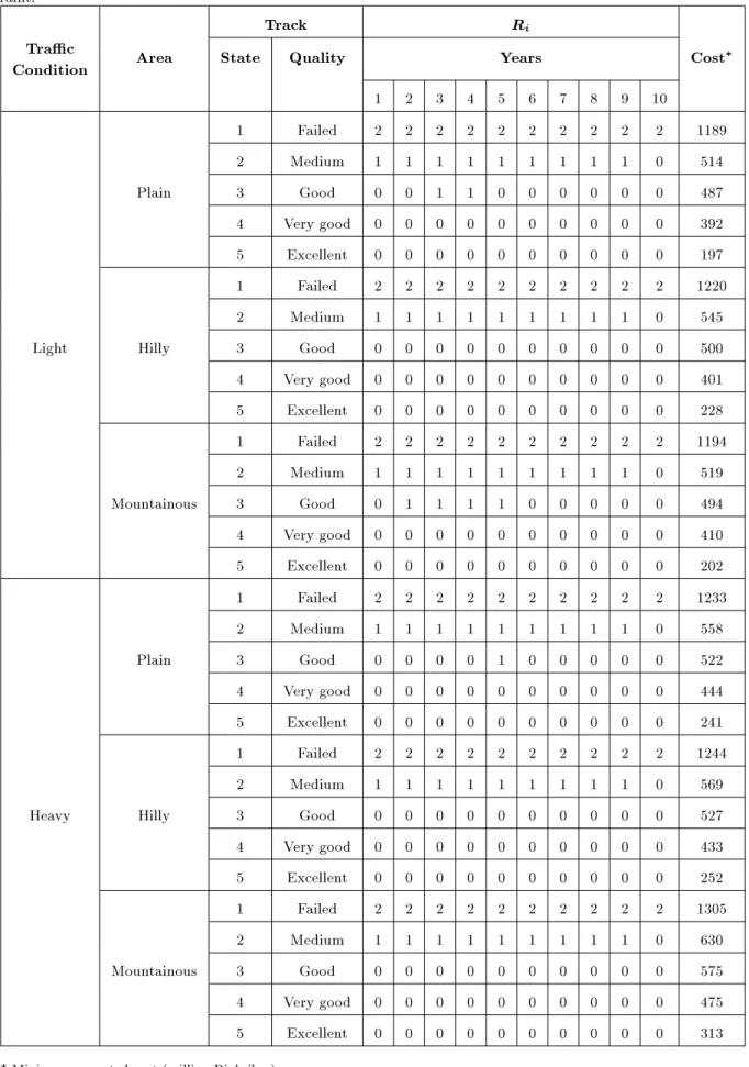
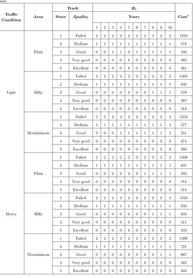
For each track class, an independent table of optimal maintenance actions and costs was computed. Any of such tables can be used as a guide to specify the optimal repair action for each possible track state in the planning horizon. The optimal maintenance actions and costs are given in Tables 7 and 8, for the non-constrained and constrained track state cases mentioned, respectively. Comparisons of the respective costs in Tables 7 and 8 show that the optimal cost for a non-constrained problem (Table 7) is less than that of a constrained problem (in Table 8), as expected. It is clear that, although there are similarities in the solution of the problem for various track classes in Table 7 or 8, such similarities cease to exist when track states extend, or repair options increase in number, or the cost structure of the repair options changes. However, such cases require more data in order to make the model operational.
CONCLUSIONS
In this study, a Markov model is presented for rail track maintenance problems, similar to work presented by Carnahan et al. [10] for road pavement management. The model proved its robustness in predicting the random behavior of the track deterioration process. The results showed that the Markov model seems to be superior to conventional regression models, such as the ORE model. Furthermore, dynamic programming demonstrated its abilities to nd optimal decisions for track maintenance systems, while minimizing the cost of maintenance. Probabilistic dynamic programming
Table 7. Optimal maintenance action and costs (million Rials/km) for 10-year horizon for tracks in the 6 classes without constraint.
Track Ri
Trac
Condition Area State Quality Years Cost
1 2 3 4 5 6 7 8 9 10
1 Failed 2 2 2 2 2 2 2 2 2 2 1189 2 Medium 1 1 1 1 1 1 1 1 1 0 514 Plain 3 Good 0 0 1 1 0 0 0 0 0 0 487 4 Very good 0 0 0 0 0 0 0 0 0 0 392 5 Excellent 0 0 0 0 0 0 0 0 0 0 197 1 Failed 2 2 2 2 2 2 2 2 2 2 1220 2 Medium 1 1 1 1 1 1 1 1 1 0 545 Light Hilly 3 Good 0 0 0 0 0 0 0 0 0 0 500 4 Very good 0 0 0 0 0 0 0 0 0 0 401 5 Excellent 0 0 0 0 0 0 0 0 0 0 228 1 Failed 2 2 2 2 2 2 2 2 2 2 1194 2 Medium 1 1 1 1 1 1 1 1 1 0 519 Mountainous 3 Good 0 1 1 1 1 0 0 0 0 0 494 4 Very good 0 0 0 0 0 0 0 0 0 0 410 5 Excellent 0 0 0 0 0 0 0 0 0 0 202 1 Failed 2 2 2 2 2 2 2 2 2 2 1233 2 Medium 1 1 1 1 1 1 1 1 1 0 558 Plain 3 Good 0 0 0 0 1 0 0 0 0 0 522 4 Very good 0 0 0 0 0 0 0 0 0 0 444 5 Excellent 0 0 0 0 0 0 0 0 0 0 241 1 Failed 2 2 2 2 2 2 2 2 2 2 1244 2 Medium 1 1 1 1 1 1 1 1 1 0 569 Heavy Hilly 3 Good 0 0 0 0 0 0 0 0 0 0 527 4 Very good 0 0 0 0 0 0 0 0 0 0 433 5 Excellent 0 0 0 0 0 0 0 0 0 0 252 1 Failed 2 2 2 2 2 2 2 2 2 2 1305 2 Medium 1 1 1 1 1 1 1 1 1 0 630 Mountainous 3 Good 0 0 0 0 0 0 0 0 0 0 575 4 Very good 0 0 0 0 0 0 0 0 0 0 475 5 Excellent 0 0 0 0 0 0 0 0 0 0 313
Table 8. Optimal maintenance action and costs (million Rials/km) for 10-year horizon for tracks in the 6 classes with constraint.
Track Ri
Trac
Condition Area State Quality Years Cost
1 2 3 4 5 6 7 8 9 10
1 Failed 2 2 2 2 2 2 2 2 2 2 1253 2 Medium 1 1 1 1 1 1 1 1 1 1 578 Plain 3 Good 0 0 1 1 0 1 1 1 1 1 546 4 Very good 0 0 0 0 0 0 0 0 0 0 462 5 Excellent 0 0 0 0 0 0 0 0 0 0 261 1 Failed 2 2 2 2 2 2 2 2 2 2 1305 2 Medium 1 1 1 1 1 1 1 1 1 1 630 Light Hilly 3 Good 0 0 0 0 0 0 0 1 1 1 579 4 Very good 0 0 0 0 0 0 0 0 0 0 487 5 Excellent 0 0 0 0 0 0 0 0 0 0 313 1 Failed 2 2 2 2 2 2 2 2 2 2 1252 2 Medium 1 1 1 1 1 1 1 1 1 1 577 Mountainous 3 Good 0 0 0 1 1 1 1 1 1 1 551 4 Very good 0 0 0 0 0 0 0 0 0 0 474 5 Excellent 0 0 0 0 0 0 0 0 0 0 260 1 Failed 2 2 2 2 2 2 2 2 2 2 1306 2 Medium 1 1 1 1 1 1 1 1 1 1 631 Plain 3 Good 0 0 0 0 0 0 1 1 1 1 592 4 Very good 0 0 0 0 0 0 0 0 0 0 515 5 Excellent 0 0 0 0 0 0 0 0 0 0 314 1 Failed 2 2 2 2 2 2 2 2 2 2 1324 2 Medium 1 1 1 1 1 1 1 1 1 1 650 Heavy Hilly 3 Good 0 0 0 0 0 0 0 1 1 1 603 4 Very good 0 0 0 0 0 0 0 0 0 0 511 5 Excellent 0 0 0 0 0 0 0 0 0 0 333 1 Failed 2 2 2 2 2 2 2 2 2 2 1396 2 Medium 1 1 1 1 1 1 1 1 1 1 721 Mountainous 3 Good 0 0 0 0 0 0 0 0 1 1 667 4 Very good 0 0 0 0 0 0 0 0 0 0 565 5 Excellent 0 0 0 0 0 0 0 0 0 0 404
could be adapted to the Markov process eciently, and constraints on track condition are easily dealt with by dynamic programming. Although there might be room for further enhancement of the model, the application of the presented model for Iranian Railways proved to be a reasonable method for the allocation of maintenance funds.
ACKNOWLEDGMENT
The authors would like to thank the Iranian Railways for the provision of data in support of this study. REFERENCES
1. Oce for Research and Experiments (ORE) \Question D161, Dynamic vehicle/track phenomena, from the point of view of track maintenance", Report no. 3, Final Report of The International Union of Railways (1988).
2. Esveld, C. \Computer-aided maintenance and renewal of track", Proceedings of the 4th International Heavy Haul Conference, Brisbane, Australia, International Heavy Haul Association Inc., Virginia Beach, VA, USA, pp. 118-123 (Sept. 11-15, 1989).
3. Zarembski, A.M. \Rail life analysis and its use in planning track maintenance", Rail Technology Inter-national, Sterling Publications Limited, pp. 211-216 (1993).
4. Zhang, Y.J. \An integrated rail track degradation model", PhD thesis, Physical Infrastructure Centre, School of Civil Engineering, Queensland University of Technology, Brisbane, Australia (2000).
5. Simson, S.A., Ferreira, L. and Murray, M.H. \Rail track maintenance planning: An assessment model",
Transportation Research Record 1713, Transportation Research Board, National Research Council, National Academy Press, Washington D.C., USA, pp. 29-35 (2000).
6. Martland, C.D., Hargrove, M.B. and Auzmendi, A.R. \TRACS: A tool for managing change", Railway Track and Structures, 90, pp. 27-29 (1994).
7. Shafahi, Y. and Rasooli, M. \A neuro networks model to predict future track condition", 6th International Conference on Civil Engineering, Isfahan University of Technology, Isfahan, Iran (2001).
8. Dell'Orco, M., Ottomanelli, M. and Sassanelli, D. \Neuro-fuzzy decision support system for rail-tracks maintenance planning", Proceedings of the 10th World Conference on Transport Research, WCTR'04, (CD-ROM version), Istanbul, Turkey (July 4-8, 2004). 9. Jovanovic, S. and Esveld, C. \ECOTRACK: An
objec-tive condition-based decision support system for long-term track M&R planning directed towards reduction of life cycle costs", Proceedings of the 7th International Heavy Haul Conference, International Heavy Haul Association Inc., Virginia Beach, VA, USA, pp. 199-207 (2001).
10. Carnahan, J.V., Davis, W.J., Shahin, M.Y., Keane, P.L. and Wu, M.I. \Optimal maintenance decisions for pavement management", Journal of Transportation Engineering, ASCE, 113(5) (1987).
11. Ayyub, B., Uncertainty Modeling and Analysis in Civil Engineering, Carol Royal, New York (1998).
12. Davidian, M. and Giltinan, D.M., Nonlinear Models for Repeated Measurement Data, Chapman & Hall, First Edition (1995).