c
Sharif University of Technology, June 2010
Prediction of Hydraulic Eciency of
Primary Rectangular Settling Tanks Using
the Non-linear k
" Turbulence Model
B. Firoozabadi
1;and M.A. Ashjari
1Abstract. Circulation is created in some parts of settling tanks. It can increase the mixing level, decrease the eective settling, and create a short circuiting from the inlet to the outlet. All above-mentioned phenomena act in such a way to decrease the tank's hydraulic eciency, which quantitatively shows how ow within the tank is uniform and quiet. So, the main objective of the tank design process is to avoid forming the circulation zone, which is known as the dead zone. Prediction of the ow eld and size of the recirculation zone is the rst step in the design of settling tanks. In the present paper, the non-linear k " turbulence model is used for predicting the length of the reattachment point in the separated ow of a Karlsruhe tank. Then, the recirculation bubble size, which is out of the capability of standard turbulence models, is determined. Also, the eect of the separation zone size on the tank's hydraulic eciency is investigated.
Keywords: Settling tanks; Non-linear k "; FTC calculation; Hydraulic eciency; Circulation.
INTRODUCTION
Settling tanks have been used for separating oating particles from the main ow. To optimize the operation of these tanks, it is required that a quiet ow of uid be formed in the tank in such a way that the sedimentation process be performed in the best way. However, creation of the dead zone and the short circuiting of the inlet to the outlet disturb the quietness of ow and leave negative inuences on the performance of the tank. To prevent these phenomena, some baes are used in several parts of the tank. By optimizing the application of the baes in the tanks, the size of the recirculation zones is reduced and the plug ow percentage, which is the ideal ow for clariers, is increased. In fact, several parameters, e.g. location and type of inow and euent, location and size of bae, and rate of sludge withdraw could inuence the eciency of settling tanks. Then, the best way to determine their order of magnitude is to develop a suitable mathematical model. Mathematical models have been mainly developed, since
incorpora-1. School of Mechanical Engineering, Sharif University of Tech-nology, Tehran, P.O. Box 11155-9567, Iran.
*. Corresponding author. E-mail: [email protected] Received 5 May 2009; received in revised form 6 December 2009; accepted 20 April 2010
tion of the standard k " turbulence model in the settling tank simulation by Rodi [1]. By using this model, researchers could simulate ow elds without any requirement of especially empirical expressions. But, Stamou et al. [2] and many other researchers have shown that obtained results through applying the standard model are only qualitatively comparable with experimental data. Only in the work of Celik et al. [3], for calculating Flow-Through Curves (FTC) of a Windsor tank, did the predicted results t excellently with experimental measurements. However, the reason for this exceptional compatibility was recognized after more consideration by Adams and Rodi [4]. In fact, introducing numerical diusion, because of using a hybrid scheme incorporated by Celik et al. [3], caused the compatibility, so their obtained results were unac-ceptable. After nding this fact, the team conducted their research on the Karlsruhe basin and tried to consider the ability of the k " model by creating more complicated ow patterns. They concluded that the standard k " model is not capable of precisely predicting the size of the recirculation zone and velocity eld in the region, which strongly aects the tank's eciency. To overcome the above weakness of the standard model, Adams and Rodi [4] carried out their calculations with a curvature modication to the k " model of Leschziner and Rodi [5]. This model had
shown good results in calculating the separation point length of backward-facing step ow. Nevertheless, overestimating the length of the recirculation zone in the tank was slightly surprising. In this ow, the formation of streamlines with strong curvature caused the modied model to work improperly.
Linear k " turbulence models, which, in fact, can be thought of as tensorially invariant mixing length theories, usually work quite well in the description of unseparated turbulent boundary layers. Although in thin shear ows, normal Reynolds stresses do not play an important role, they have a main role in describing ows that involve recirculation zones. In these cases, incorporating the linear k " models, which are completely incapable of accurately predicting normal Reynolds stresses, is not a very appropriate model.
Preliminary research taking into account the ef-fects of non-linear terms and modifying the k " model was undertaken by Launder and Ying [6] and Rodi [7]. However, the obtained models were developed in such a way that general invariance was not exhibited and, hence, good results only showed for special ows. It is very interesting that the main steps in developing a general non-linear turbulence model had been taken many years ago by Rivlin [8] and Lumley [9]. They had focused on a clue whereby there exist striking similarities between the main turbulent ow of a New-tonian uid and the laminar ow of viscoelastic uids. Continuation of their method by further researchers caused the desired model, known as non-linear or anisotropic k ", to be obtained by Speziale [10]. A few years later, Launder [11] oered a very complete form of the model that contained higher order terms. In addition, these non-linear models have all advantages of the linear k " model; they can better describe the normal stresses and can be incorporated into most k " model computer codes in a relatively simple manner.
In this paper, some numerical problems that occur through the appearance of non-linear terms in the anisotropic turbulence model will be introduced. In addition, the size of the recirculation bubble in the Karlsruhe basin will be determined by using the non-linear k " model and comparing it with Adams and Rodi's [4] experimental measurements. Finally, the performance of the non-linear model in predicting the hydraulic eciency and FTC of the tank, which are strongly aected by the velocity eld and recirculation size, will be investigated.
MATHEMATICAL MODEL
The steady state, two-dimensional ow in the Karl-sruhe basin is determined using time averaged conser-vation equations. The Navier-Stokes and continuity equations for Newtonian incompressible uid are
ex-pressed as: @u @x+
@v
@y = 0; (1)
u@u @x+ v
@u @y =
@ ~p @x+
@2u @x2 +
@2u @y2
@11 @x
@12
@y ; (2)
u@v@x+ v@v@y = @x@ ~p+
@2v @x2+
@2v @y2
@12 @x
@22
@y : (3)
where u and are the mean velocity components in the x and y directions; ~p is the modied mean pressure dened by Speziale and Thangam [12]; 11, 22 and 12 are normal and shear components of the Reynolds stresses, respectively, and is the kinematic viscosity of the uid (here, it is water at 20C). The Reynolds stresses could be modeled via an eddy viscosity assumption based on Speziale [10] in the form:
ij =23kij 2Ck 2
" Sij 4CDC2k 3 "2
So
ij 13Skko ij+ SikSkj 13SklSklij
; (4) where subscripts i; j = 1 and 2 stand for x and y, respectively; k is the kinetic energy of turbulence; " is the turbulent dissipation rate, and C is a dimen-sionless constant that is taken to be 0.09, as oered by Rodi [1]. CD is the dimensionless constant, dened as 1.63, based on calibration of the non-linear model with Laufer's [13] experimental data for fully developed turbulent channel ow; ij is the Kronecker delta, and Sij, the mean rate of strain tensor, is expressed by:
Sij =12
@ui @xj +
@uj @xi
; (5)
So
ij is the frame-indierent Oldroyd derivative deter-mined by :
So
ij = uk@S@xij k
@ui @xkSkj
@uj
@xkSki: (6)
It is clear that at the limit of CD ! 0, the standard k " model is recovered from the non-linear model. This is the same as the eective viscosity hypothesis of Boussinesq, which relates the Reynolds stresses solely to the rates of strain of the uid. This formula has been used with considerable success by Ng [14] and Rodi [15] for free shear ows, in conjunction with
turbulence models, for k and ". It has been observed, however, that the Boussinesq hypothesis fails in a number of applications, such as separated turbulent ows. Bradshow [16] has stated that this failure is due to the form of the stress strain relation rather than the inapplicability of the eddy viscosity approach. In particular, the third term in Equation 4 corrects the fundamental weaknesses of the Boussinesq relationship. As shown by Pope [17], the new relationship has a strong ability to capture normal stress anisotropy, high sensitivity to secondary strains, and an ability to generate excessive turbulence at separation zones. Detailed tests by Speziale [10], Suga [18], and Craft et al. [19] have shown that the eect of the last term in Equation 4 is a signicant improvement in the prediction of the reattachment length of the separation region behind the backward facing step, with results similar in accuracy to those obtained using a Reynolds stress model. However, the main advantage of the non-linear model over more sophisticated turbulence models is that the time consuming solution of the stress equations, in the form of partial dierential or algebraic, is not needed. In addition, the inter-relation between strain and stress has been retained within the dierential equation, which increases the numerical stability of the model. Our numerical experiences have shown that the non-linear model of Speziale [10] has a strong capability of predicting separated ow within settling tanks, while its numerical implementation and stability is, approximately, as simple and as good as the standard model. Nevertheless, some ner grids and, consequently, more CPU time are needed to deal with non-linear terms.
It is worth mentioning that k and ", in the non-linear model, are calculated using the same transport equations incorporated in the standard k " model [1]. Through Equations 1 to 6, the ow eld in the basin could be solved and, hence, the tank's model is fully dened hydrodynamically. To complete the tank's modeling, the determined velocity eld must be introduced into the transport equation of the dye such that the concentration can be calculated. By supposing that the dye has no inuence on the ow eld, and is dispersed only via diusion and convection mechanisms, the transport equation will be:
@C @t +
@uC @x +
@vC @y =
@ @x
t@C@x
+@y@
t@C@y
; (7) where C is the mean dye concentration and t, the isotropic eddy diusivity coecient, is proportional to the eddy viscosity, t=tc, according to the Reynolds analogy theory for mass and momentum transport. Here, proportional coecient cis the Schmidt number and is 0.7, as proposed by Launder [11], for free turbulent ows.
INITIAL AND BOUNDARY CONDITIONS The hydrodynamics part of the problem is steady state and the initial condition for the velocity eld is not very important. Nevertheless, for calculating the tank's FTC, no dye must exist, initially, all over the tank (C = 0).
By knowing the velocity at the rst node above the solid boundary, the shear velocity is calculated via the law of the wall, in the standard two-layer form developed by Launder and Spalding [20], and the wall is taken as being smooth. Formally, the wall function must not be applied to separated-turbulent boundary layers, and many researchers like Avva et al. [21] tried to modify it in several ways. However, since the ow eld is solved iteratively, and the separated regions occupy a small space, conned only at the tank corner, major errors do not appear to the overall ow eld. After calculating the shear velocity, the values of k and " at the adjacent node above the wall are determined by assuming local equilibrium for turbulent production and dissipation [1]. All boundary conditions at the inlet, outlet, and free surface of the model tank are applied as recommended by Celik et al. [3].
NUMERICAL SOLUTION PROCEDURE A new computer code, in FORTRAN 90, is developed to solve hydrodynamics and mass distribution equa-tions, numerically. The use of staggered grids and a control volume method is the main characteristic of the new code. However, the pressure eld is corrected at each step by the SIMPLEC algorithm introduced by Patankar [22]. To enhance numerical stability, the convection terms are approximated by using a hybrid (upwind/central) scheme. In addition, an under-relaxation factor for all dependent variables must be taken to control the strong tendency for divergence. Nevertheless, as the turbulent production term in transport equations for k and " [1] is non-linear and the velocity gradients at primary steps are so digressive, the eddy viscosity must be limited to less than 2500 and under-relaxed in each itera-tion.
To ensure that the non-linear turbulence model is applied correctly in the new code, a fully developed turbulent ow in a channel, as a simple test case, is simulated. The normal stresses obtained by the code using dierent models are compared with experimental data of Laufer [13] in Figure 1. In contrast with the non-linear model, the linear model has the same estimation of both normal stresses. These results simultaneously validate both the non-linear model and the developed code itself.
In order to discretize Equation 4, it is required that the Reynolds stresses be determined at the main
Figure 1. Normal Reynolds stresses in fully developed turbulent channel ow.
nodes where ~p; "; k; and C are stored. But, at the main nodes near the boundary, the Oldroyd derivative terms could not be approximated via a central dierence scheme, which has a second-order error. Hence, the Reynolds stresses are extrapolated there. The validity of this simplication could be explained by noting the general behavior of turbulent ows near the boundary and linear variations of the stresses, there, in fully developed turbulent channel ows (Figure 1). In addi-tion, for the staggered grid [23] used in the calculations, the shear stresses must be known at the cell faces instead of the main nodes where scalar variables are stored. Interpolating could easily solve this problem, but the stress consistency between the two adjacent cells must not be forgotten. This means that four surrounded main nodes are required to interpolate the shear stress at the cell face.
To control the strong divergence, because of the application of the non-linear k " model, two strategies are taken into account in the solution. First, the calculated ow eld, by the linear k " model, is introduced as an initial condition. Second, the eects of non-linear terms in the anisotropic model are gradually contributed to the solution process by imposing a limitation condition on them. The upper bound of this limitation is dened by comparing the non-linear terms with their corresponding linear terms (i.e. two right hand side terms) in Equation 4. It is worth noting that the modied terms in Equation 4 have more dispersive features than the favorable dissipative one. Thus, in solving the ow eld, by using the non-linear k ", and with the initial condition obtained by the standard k ", the averaged-mean-square errors resulting from mass imbalances in control volume will not be drastically reduced. Hence, the calculation process is continued until the dierence in length of
the separation point of the successive iterations is less than 1%.
In order to calculate the FTC of the tank, Equa-tion 7 is discretized using a fully implicit time dis-cretization method proposed by Roache [24]. Although this method is only rst order, an accurate calculation could be achieved by choosing a reasonable time step, which should be determined case by case. Nevertheless, dominant errors of approximating convection terms which have shown themselves as \so called numerical or false diusion" are still present, which virtually increase the physical diusion. In fact, as Roache [24] has shown, the solved dierence equations will give the solution of the equation below instead of Equation 7, when convection terms are approximated by using the hybrid scheme:
@C @t +
@uC @x +
@vC @y =
@ @x
( t+ num)@C@x
+@y@
t@C@y
+ HOT; (8)
where HOT stands for Higher-Order Terms. num is the numerical diusivity from the numerical approxi-mation errors. Numerical diusion is neglected in the y direction in Equation 8 because the ow in the tank is nearly unidirectional and the cross-stream convection is small.
A practical way to eliminate any numerical diu-sion, especially in unsteady problems, is to incorporate more accurate dierencing schemes. However, using higher-order schemes has caused stability problems often called wiggles in literature, which limit the application of more accurate schemes. So, as a rst approximation, the most popular second-order QUICK is recognized as being suitable for the FTC calculation of the Karlsruhe tank. In addition, due to an increase in the bandwidth of the linear equations system by using the standard QUICK scheme of Leonard [25] the QUICK scheme of Hayase et al. [26] is used here. FLOW FIELD PREDICTION USING THE MODEL
Figure 2 shows the dimensions of the Karlsruhe model tank, which is selected for ow consideration at Re = 10000 (dened with respect to hi, inlet slot high). Its experimental measurements were given by Adams and Rodi [4].
For ow computations of the surface discharge case, Si=h = 0:91, a 75 35 grid was sucient to give grid independent solutions. This could be further examined through Figure 3, which shows root mean square errors in dierent entrance cross sections for u-velocity and eddy viscosity proles. Errors for any
Figure 2. Dimensions of Karlsruhe basin; in surface discharge case Si= 10 cm and in submerged discharge
case Si= 6:468 cm.
Figure 3. u-velocity and eddy viscosity error in dierent cross sections for surface discharge case. (a) Linear; (b) Non-linear model (E(X) =
s
1 N
N
P
1(X Xref) 2).
examined grid are calculated relative to a selected reference grid, for instance 150 70. A solution is considered grid independent if its error drops below a prescribed value, chosen here as 0.02. According to this criterion, a 75 35 grid is suciently ne for both linear (Figure 3a) and non-linear (Figure 3b) models. Figure 4a shows the streamlines by using a
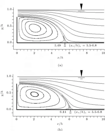
Figure 4. Calculated ow eld with 75 35 grid for surface discharge case. (a) Linear k "; (b) Non-linear k ".
linear k " model. The reattachment length is the same as that reported by Adams and Rodi [4]. This predicted length is only at the lower range of the experiments (xr=h = 5:5 6:5). This can be related to the incapability of the linear model. In contrast, in the ow eld, which is calculated by non-linear k ", as illustrated in Figure 4b, the length of the separation point is increased and reaches xr=h = 6:14. This is now in the experimental range completely and shows clearly the eectiveness of the applied model.
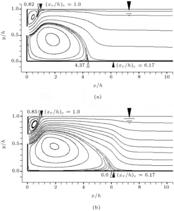
However, the performance of the non-linear model could be seen more obviously if the submerge discharge case, Si=h = 0:588, is considered. Due to the complication of this ow, a grid independent solution is not achieved for both linear and non-linear models with the same grid size (Figure 5). This can also be seen in Figures 6 and 7 that show the calculated streamlines with two dierent grids. Although using a ner grid with the linear k " has not caused much dierence in the ow eld (Figures 6a and 7a), the dierence in the size of the recirculation bubble is considerable in the case of the non-linear model (Figures 6a and 6b). Therefore, it is inferred that when the non-linear k " is applied for a complicated ow eld, the corresponding size of the grid must be about four times greater than the size of a grid that was given a grid independent solution with the linear k " model. This will cause the computation time for the non-linear
Figure 5. Error of u-velocity and eddy viscosity in dierent entrance cross sections for submerged discharge case. (a) Linear and (b) Non-linear k " model
(E(X) = s
1 N
N
P
1(X Xref) 2).
model to be dramatically increased. Table 1 shows that when the same grid is used for both models (in surface jet), the non-linear model has a computational time approximately two times greater than the linear model. However, for a submerged jet, a ner grid is required for the non-linear model, so that it has about 30 times greater computational time. This could only be justied in cases where high accuracy is needed e.g. in tank performance calculations (next section).
For the case Si=h = 0:588, two small and large separation zones exist in the ow. Their calculated length, using two models, is compared in Figure 7. Although the modication in the size of the upper small separation zone is not so noticeable, the size of the lower large separation zone is increased from xr=h = 4:37, for linear k ", to xr=h = 6:0, for non-linear k ", and well approaches the experimental value (xr=h)e = 6:17. Hence, the non-linear model, without any regard to the ow type and its
com-Figure 6. Computed streamlines with 75 52 grid for submerged discharge case. (a) Linear model; (b) Non-linear model.
Figure 7. Computed streamlines with 150 100 grid for submerged discharge case. (a) Standard k "; (b) Non-linear k ".
Table 1. Computational time and separation length error of dierent grids.
Surface Discharge Case Grid Size Linear k "
xr=h Reattachment
Length Error
CPU Times (s) 19 9 5.10 9.0% 8 38 18 5.39 3.7% 38 75 35 5.49 2.0% 646 150 70
(Reference) 5.6 0.0% 9267 Non-Linear k "
19 9 5.65 8.9% 17 38 18 6.04 2.6% 77 75 35 6.14 1.0% 892 150 70
(Reference) 6.20 0.0% 18780 Exp.
Adams et al. [4]
6.4 | |
Submerged Discharge Case Grid Size Linear k "
xr=h Reattachment
Length Error
CPU Time (s) 38 26 3.2 27.0% 74 75 52 4.32 1.3% 878 150 100 4.37 0.2% 13210 300 200
(Reference) 4.38 0.0% 88122 Non-Linear k "
38 26 3.83 36.7% 135 75 52 5.18 14.4% 1700 150 100 6.00 0.8% 25000 300 200
(Reference) 6.05 0.0% 190000 Exp.
Adams et al. [4]
6.2 | |
plexity, acts quite well in predicting the size of large recirculation zones, which are more interesting. The model only fails in simulating small recirculation zones where the curvature of streamlines is extraordinarily strong. These small separation bubbles are not more important, as they have negligible inuence on the ow characteristics.
The reason why the standard turbulence model is unsuccessful in predicting separated ows will be clearer when momentum equations are written in terms of the mean ow stream function, , (where u = @ @y
and v = @ @x) as: u @
@x r2
+ v @ @y r2
= ( + t) r4 @2(22 11)
@x@y
@212 @x2 +
@212 @y2 : (9) This equation shows that in cases where high velocity gradients are present, the linear k " model is unable to predict the normal Reynolds stress dierence, 22 11. This term contributes directly to calculating the streamlines and their curvatures. It can be shown that the linear model predicts the sum of the normal Reynolds stresses as (11 + 22 = 233), for any 2-D ows, that surely will not satisfy all cases. In other words, the linear model has some problems in calculating the normal stresses.
Figure 8a compares the measured and calculated dimensionless streamwise velocity, u=uin, at several critical sections in the recirculation zone for the sub-merged discharge case (the case in which the inlet ow is from the middle height of the tank). The superiority of the non-linear model, especially in the regions near the separation point, x=h = 5:58, 5:88 and 6:17, is clearly apparent. Furthermore, Figure 8b gives additional information about the status of turbulence
Figure 8. Dimensionless velocity (a) and turbulence kinetic energy (b) proles at several critical sections in recirculation zone of Karlsruhe tank in submerged discharge situation.
in the tank. In this gure, the calculated dimensionless turbulence kinetic energy (divided by the square mean inlet velocity, u2
in) using both standard and non-linear k " models, is compared with the experimental data of Adams and Rodi [4]. As expected, the highest turbulence levels are found in shear layers bordering the separation zones (i.e. x=h < 6:2). Beyond reattachment, the turbulence level drops quickly to about a constant small value due to the absence of any signicant velocity gradients. This simply explains why the standard k " model has very poor predictions of turbulence kinetic energy levels within the separation zone, while having a good performance out of this region. As shown earlier, the section, x=h = 5:58, for a submerged discharge case, is entirely out of the separation region when the linear k " model is incorporated. In contrast, the separation zone has extended beyond this station for the non-linear k " model and for measurements. Therefore, nearly good agreement is observed between the non-linear k " model and experimental data for this critical section. However, separation has ended at this section and, consequently, the turbulence level has dropped for the linear k " model.
CALCULATING THE FTC
The hydrodynamic performance of a tank is obtained by injecting uorescent dye with the same density as the internal water at a denite time in the inlet and measuring the outlet dye concentration several times. A curve that shows the dye concentration variation in the outlet with time is called a Flow-Through Curve (FTC). It is more convenient to present the FTC with dimensionless variables. Hence, time is non-dimensionalized by the theoretical detention time, Tth = hlq , where q is the inlet ow rate, and concentration by Co= mhlin, where minis the total mass of the dye to enter the tank.
To calculate the FTC of the Karlsruhe tank, the concentration transport Equation 7 must be solved by introducing the computed ow eld in the previous section. In addition, for simplicity, the inlet boundary condition is taken as C = 1 during the injection time and C = 0 for the next times.
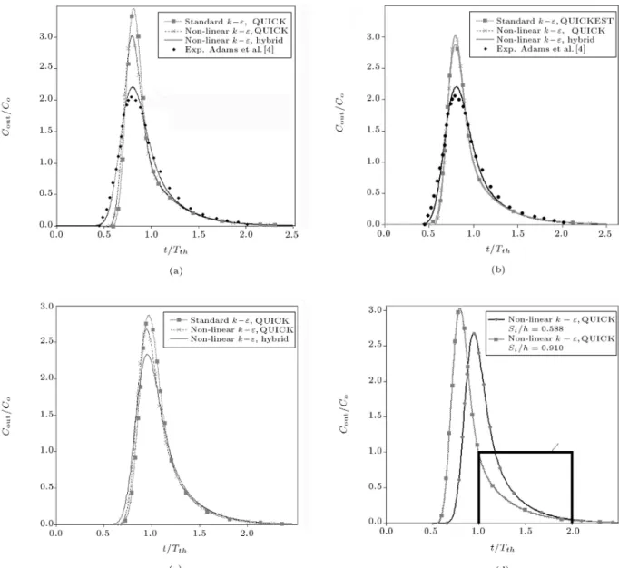
Figure 9a compares the calculated FTC for a surface discharge situation, with both hybrid and QUICK schemes, using two dierent ow elds ob-tained by linear and non-linear models, with Adams and Rodi's [4] measurements. In this case, the peak concentration predicted with the hybrid scheme and non-linear k " model is almost the same as that measured, while the peak concentration predicted by the QUICK scheme and the non-linear k " model is about 35% higher. However, this value is more
(about 60%) when a linear k " model is used. The discrepancy between the numerically accurate QUICK calculation and the measurements may be due to three reasons. The rst possibility is that the incorporated turbulence model in the hydrodynamic part cannot produce sucient mixing, i.e. eddy diusivity as it is produced in the experiment. According to Figure 9b, this is the case, but it does not solely justify the poor prediction of the QUICK scheme. The level of the turbulence uctuations predicted by the linear k " model is generally lower than the measurements and the non-linear turbulence model. Therefore, the FTC calculation for the ow eld obtained by the non-linear k " model can reduce peak concentration to about 25%. This is high, but not as much as expected. The second possibility for the dierence in peak concentration may be due to the inconsis-tency of the QUICK scheme with the physics of the problem. The QUICK scheme is often used in steady state calculations (also it has been used for transient computations by some researchers), while many other schemes have been proposed originally for transient calculations. To discover the eect of unsteadiness in the calculations, we have repeated the FTC calculation with the third order accurate QUICKEST scheme developed originally by Leonard [25]. To avoid the oc-currence of non-physical numerical oscillations, a mod-ied ULTIMATE algorithm has also been used [27]. The result (Figure 9b) is observed as a lowering in peak concentration by an amount of 8% relative to the QUICK scheme. Hence, another possibility may also exist. Based on the statements of Adams and Rodi [4], three-dimensional motions were observed in the experimental tank, in spite of their attempt to keep the motion two-dimensional through the large aspect ratio of the tank. Denitely, additional mixing due to these three-dimensional motions is not reproducible by using the two-dimensional model.
Figure 9c, for a submerged discharge case, shows that the peak concentration is highest for the linear k " with the QUICK scheme and lowest for the non-linear model with the hybrid scheme. In this situation, when the size of the recirculation zone is enlarged, the peak concentration decreases, as shown previously. But, the passing time of peak concentration decreases.
Figure 9d shows a comparison between the FTC of the two dierent cases, which were calculated using precise ow elds and a QUICK scheme without nu-merical diusion. In the submerged discharge case, the FTC is changed in such a way that it approaches the ideal step FTC that could be considered as a sign of higher hydraulic eciency.
Through the FTC, some important parameters, such as the level of short-circuiting, the mixing level inuenced by both diusion and/or recirculation zones,
Figure 9. FTC for (a, b) surface and (c) submerged, discharge cases and (d) comparison with each other.
and overall eciency, could be calculated. The time it takes for the rst dye to appear at the outlet is dened as the short-circuiting level and is shown by t0and t10 indices (tn is the time which takes until n percent of the total injected dye into the tank is passed through the outlet). The value of these indices depends on both the ow eld and the mixing level. When the values are low, one may conclude that short-circuiting exists and it shows a false designing of the tank. The mixing level in the tank, dened by t75 t25, t90 t10 and t90=t10, is increased by increasing the diusion coecient and the size of the recirculation bubble. Nevertheless, the performance of the tank is increased by the former and decreased by the latter. t50and tmax, the passing time of peak concentration, are indices to express the overall eciency of the tank.
All the computed FTC characteristic indices of the Karlsruhe tank are summarized in Table 2. The
short-circuiting indices are decreased or, in other words, the level of short-circuiting is increased by increasing the separation bubble (compare columns 1 with 2 or 4 with 5) and the virtual diusion coecient created by additional numerical diusion (compare columns 2 with 3, or 5 with 6). In addition, Table 2 shows that the tank's mixing level is increased when the above-mentioned factors increase. This high mixing disturbs the still circumstances, which are required for ecient settling. Altogether, it is inferred from Table 2 that increasing the recirculation size causes a high level of short circuiting and mixing. The result of these complicated events can be seen on the reduction of t50 and tmax indices that indicate tank performance. Conversely, the eciency of the tank is not more sensitive to the diusion coecient; however, the mixing level in the tank is increased by its increasing (see columns 2, 3 or 5, 6 of Table 2).
Table 2. FTC indices of Karlsruhe tank.
Si=h = 0:588 Si=h = 0:91
FTC Index
Standard k " Quick
Non-Linear k " Quick
Non-Linear k " HYBRID
Standard k " Quick
Non-Linear k " Quick
Non-Linear k " HYBRID
Exp. Adams et al. [4] Short
Circuiting
t0 0.67 0.653 0.59 0.62 0.584 0.407 0.45
t90 0.865 0.843 0.828 0.73 0.713 0.66 0.65
Mixing
t75 t25 0.225 0.258 0.276 0.228 0.253 0.307 0.32
t90 t10 0.513 0.577 0.601 0.554 0.604 0.679 0.59
t90=t10 1.593 1.684 1.726 1.755 1.847 2.029 1.91
Eciency
tmax 0.965 0.942 0.953 0.811 0.797 0.797 0.78
t50 1.023 1.01 1.018 0.862 0.859 0.872 0.87
CONCLUSION
This paper has presented the main reasons for de-ciency in the standard k " turbulence model in prediction of the separation point length of the ow in the Karlsruhe tank. The non-linear k " model was used to overcome the weakness of the linear model and to calculate the size of the recirculation zone exactly. Comparing the computed streamwise velocity proles with measurement data in several critical sections shows that the non-linear model is more eective. In addition, incorporating the velocity elds, obtained by the two dierent turbulence models, shows that a precise ow eld is the main requirement for calculating an accurate FTC. If the size of the separation bubbles in the Karlsruhe is predicted slightly larger, a reduction will appear in the tank's overall eciency. However, this reduction is not very notable because the size of the recirculation zone is small, with respect to the tank's volume, and strong 3-D eects were present in the tank.
To consider the complicated eects of the recir-culation zones, the non-linear k " model was used to calculate the FTC. This is reasonable because the non-linear model has no increased computation costs and can be incorporated simply into codes with the standard k " model.
ACKNOWLEDGMENT
The authors would like to express their gratitude and sincere appreciation to Dr. M.T. Manzari, associate professor of Sharif University of Technology for his valuable comments to overcome the numerical prob-lems of this project.
NOMENCLATURE
C mean dye concentration
Co reference concentration
CD coecient of non-linear terms in Reynolds stresses formula
C"1; C"2 experimental constants in " transport equation
C dimensionless constant in Reynolds stresses formula
E(X) root mean squares error of variable X in a selected cross section
h depth of basin
hi width of inlet slot
k kinetic energy of turbulence
L length of basin
min total injected mass of dye
n normal distance from the solid wall N number of data in each cross section to
calculate E(X) ( 20)
P turbulence production term
~p modied mean pressure
q inlet ow rate
Re Reynolds number dened with respect to inlet slot high
Si location of inlet slot above tank bottom Sij mean rate of strain tensor
So
ij frame-indierent Oldroyd derivative Tth theoretical detention time
t time
u; v mean velocity components in the x and y directions
uin inlet velocity
x; y streamwise and vertical direction xr separation point length
yp normal distance to the wall from wall adjacent grid point
ij Kronecker delta
t isotropic eddy diusivity coecient num numerical diusivity
" turbulent dissipation rate
kinematic viscosity
t isotropic eddy viscosity
c turbulent Schmidt number for dye "; k Schmidt number for k and " xx; yy normal components of Reynolds
stresses
xy shear component of Reynolds stress mean ow stream function normalized by ow rate (q)
Subscripts
1; 2 x and y directions, respectively n percent of total injected dye which has
passed through outlet
e experimental data
ref selected reference grid REFERENCES
1. Rodi, W. \Turbulence models and their application in hydraulics", Int. Association of Hydr. Res., Delft, The Netherlands (1980).
2. Stamou, A.I., Adams, E.W. and Rodi, W. \Numerical modeling of ow and settling in primary rectangular clariers", J. Hydraulic Research, 27(5), pp. 665-682 (1989).
3. Celik, I., Rodi, W. and Stamou, A.I. \Prediction of hydrodynamic characteristics of rectangular settling tanks, turbulence measurements and ow modeling", ASCE, New York, NY (1985).
4. Adams, E.W. and Rodi, W. \Modeling ow and mixing in sedimentation tanks", J. Hydraulic Engineering, 116(7), pp. 895-913 (1990).
5. Leschziner, M.A. and Rodi, W. \Calculation of annular and twin parallel jets using various discretization schemes and turbulence model variations", J. Fluids Engineering, ASME, 103, pp. 252-260 (1981). 6. Launder, B.E. and Ying, W.M. \Fully developed
turbulent ow in ducts of square cross section", Rep. TM/TN/A/11. Imperial College of Science and Tech-nology (1971).
7. Rodi, W. \Example of turbulence models for incom-pressible ows", AIAA J., 20, pp. 872-879 (1982). 8. Rivlin, R.S. \The relation between the ow of
non-Newtonian uids and turbulent non-Newtonian uids", Q. Appl. Maths., 15, pp. 212-214 (1957).
9. Lumley, J.L. \Toward a turbulent constitutive rela-tion", J. Fluid Mechanics, 41, pp. 413-434 (1970). 10. Speziale, C.G. \On nonlinear k l and k " models
of turbulence", J. Fluid Mechanics, 178, pp. 459-475 (1987).
11. Launder, B., Lectures in Turbulence Models for Indus-trial Applications, Summer School in Germany (1993). 12. Speziale, C.G. and Thangam, S. \Turbulence ow past a backward-facing step: A critical evaluation of two-equation models", AIAA J., 30(5), pp. 1314-1320 (1992).
13. Laufer, J. \Investigation of turbulent ow in a two-dimensional channel", NACA Report 1053, Washing-ton (1951).
14. Ng, K. \Predictions of turbulent boundary-layer devel-opments using a two-equation model of turbulence", PhD Thesis, University of London, UK (1971). 15. Rodi, W. \The prediction of free turbulent boundary
layers by use of a two equation model of turbulence", PhD Thesis, University of London, UK (1972). 16. Bradshaw, P. \Turbulence: the chief outstanding
diculty of our subject", J. Experiments in Fluids, 46, pp. 203-216 (1994).
17. Pope, S. \A more general eective-viscosity hypothe-sis", J. Fluid Mechanics, 72, pp. 331-340 (1975). 18. Suga, K. \Development and application of a non-linear
eddy viscosity model sensitized to stress and strain invariants", PhD Thesis, Department of Mechanical Engineering, UMIST, Manchester (1996).
19. Craft, T., Launder, B.E. and Suga, K. \Development and application of a cubic eddy-viscosity model of turbulence", Int. J. Heat Fluid Flow, 17, pp. 108-115 (1993).
20. Launder, B.E. and Spalding, D. \The numerical com-putation of turbulent ows", Comp. Methods Appl. Mech. Eng., 3, pp. 269-289 (1974).
21. Avva, R.K., Kline, S.J. and Ferziger, J.H. \Computa-tion of the turbulent ow over a backward-facing step using the zonal modeling approach", AIAA, paper 88-0611 (1988).
22. Patankar, S.V., Numerical Heat Transfer and Fluid Flow, Hemisphere Publishing Corporation, Taylor & Francis Group, New York (1980).
23. Versteeg, H.K. and Malasekera, W., An Introduction to Computational Fluid Dynamics-The Finite Volume Method, Longman Group, London (1995).
24. Roach, P.J., Computational Fluid Dynamics, Hermosa Publishing, Albuquerque, N.M. (1972).
25. Leonard, B.P. \A stable and accurate convective mod-eling procedure based on quadratic upstream interpo-lation", Comput. Methods Appl. Mech. Eng., 19, pp. 59-98 (1979).
26. Hayase, T., Humphrey, J.A.C. and Greif, R. \A consistently formulated QUICK scheme for fast and stable convergence using nite-volume iterative calcu-lation procedures", J. Comput. Phys., 98, pp. 108-118 (1990).
27. Wu, Y. and Falconer, R.A. \Rened two-dimensional ULTIMATE QUICKEST scheme for conservative so-lute transport modeling", Proceedings of Third Inter-national Conference on Hydro-Science and Engineer-ing, Cottbus/Berlin, Germany, 1, pp. 1-13 (1998).
BIOGRAPHIES
Bahar Firoozabadi is associate professor in the school of mechanical engineering at Sharif University of Technology, Tehran. Her research interests are
uid mechanics in density currents, presently focusing on bio uid mechanics, and porous media. She received her PhD in mechanical engineering also at Sharif University. She teaches uid mechanics and gas dynamics for undergraduates, and viscous ow, advanced uid mechanics, continuum mechanics and biouid mechanics for graduate students.
Mohammad Ali Ashjari was born in 1977 at Tabriz, centre of East Azarbayjan province, Iran. His academic program has been started since 1996 when he has entered Tabriz University to study Mechanics of Fluids. He had continued his education in Sharif University of Technology (SUT) in M.Sc. degree. He has received PhD degree in Thermo-Fluid from SUT in 2008. Dr. Ashjari's interest research eld is developing and introducing novel numerical methods for uid ow simulation under complicated conditions including turbulence and multi-phase porous media. He is now faculty member of Jolfa's Azad University.