ISSN: 2322-1666 print/2251-8436 online
NEW APPROACH FOR SOLUTION OF VOLTERRA INTEGRAL EQUATIONS USING SPLINE
QUASI-INTERPOLANT
MARYAM DERAKHSHAN KHANGHAH AND MOHAMMAD ZAREBNIA
Abstract. In this paper, we present quadratic rule for
approxi-mate solution of integrals using spline quasi-interpolant. The method is applied for solving the linear Volterra integral equations. Also the convergence analysis of the method is given. The method is applied to a few examples to illustrate the accuracy and implementation of the method.
Key Words: Spline; Quasi-interpolant; Volterra; Convergence.
2010 Mathematics Subject Classification:65R20; 41A15; 41A25.
1. Introduction
Integral and integro-differential equations are mathematical tools in many branches of science and engineering. The numerical methods for linear integral equations of the second kind studied in Delves [6]. Among these equations, Volterra integral equations arise from multiple appli-cations, for example physics and engineering such as potential theory, Dirichlet problems, electrostatics, the particle transport problems and heat transfer problems [3, 9]. Several numerical methods have been considered to approximate the solution of Volterra integral equations such as the papers [1,4, 5, 7, 10] that are concerned respectively with rational basis functions with product integration methods, collocation
Received:22 December 2019, Accepted: 1 August 2020. Communicated by Nasrin Eghbali ∗Address correspondence to Maryam Derakhshan; E-mail: M.Derakhshan @uma.ac.ir
c
⃝2019 University of Mohaghegh Ardabili.
methods in certain polynomial and polynomial spline spaces with uni-form and graded meshes, the generalized Newton-Cotes uni-formulae com-bined with product integration rules, mathematical programming meth-ods and fractional linear multistep methmeth-ods. In [17], Riley approxi-mated the Volterra integral equations by sinc approximation methods. Reihani have solved Fredholm and Volterra integral equations by ratio-nalized Haar functions method [16]. Simpson’s quadrature method [13], Galerkin method with the Chebyshev polynomials [15] and repeated Simpson’s and Trapezoidal quadrature rule [2] are other works on de-veloping and analyzing numerical methods for solving Volterra integral equations.
Moreover, one can refer to other methods such as [14, 19, 20]. The linear Volterra integral equation is considered as
(1.1) u−Ku=g,
where linear integral operator K is defined as
(1.2) (Ku)(x) =
∫ x a
k(x, t)u(t)dt,
g(x) andk(x, t) are known continuous functions andu(x) is the unknown function to be determined. Integration of a function is an important operation for many physical problems.
The organization of the paper is as follows. In Section 2, we describe the construction of quadrature rule based on spline quasi-interpolant. In Section 3, we give an application of the quadrature rule of Section 2 to the numerical solution of Volterra integral equations. In Section 4, the convergence and error analysis of the numerical solution are provided. At the end we give some numerical examples which confirm our theoretical results.
2. Quadrature rule based on a quadratic spline quasi-interpolant
Let Xn :={xk, 0 ≤k ≤n} be the uniform partition of the interval
I = [a, b] into n equal subintervals, i.e. xk := a+kh, with h = b−na. We consider the space S2 = S2(I, Xn) of quadratic splines of class C1 on this partition. Canonical basis is formed by the n+ 2 normalized B-splines, {Bk, k ∈J}, J :={1,2,· · ·, n+ 2}. Consider the quadratic spline quasi-interpolant (dQI) of a function f defined onI and given in
[18], that is
(2.1) ϕ2f =
∑ k∈J
υk(f)Bk,
where
υ1(f) =f1, υn+2(f) =fn+2,
υ2(f) =−1/3f1+ 3/2f2−1/6f3 =β1f1+β2f2+β3f3,
(2.2) υn+1(f) =−1/6fn+3/2fn+1−1/3fn+2=β3fn+β2fn+1+β1fn+2, and for 3≤j ≤n,
(2.3) υj(f) =−1/8fj−1+ 5/4fj−1/8fj+1 =γ1fj−1+γ2fj+γ3fj+1, withfi =f(ti), t1 =a, tn+2 =b, ti=a+ (i−3/2)h, 2≤i≤n+ 1.The quadratic B-spline functions at knots are defined as
Bi(x) =
(x−xi−3)2
(xi−1−xi−3)(xi−2−xi−3), xi−3 ≤x < xi−2, (xi−x)(x−xi−2)
(xi−xi−2)(xi−1−xi−2) +
(x−xi−3)(xi−1−x)
(xi−1−xi−3)(xi−1−xi−2), xi−2 ≤x < xi−1, (xi−x)2
(xi−xi−2)(xi−xi−1), xi−1 ≤x < xi. We consider the quadrature rule defined by
(2.4) Iϕ2f(x) :=
∫ x
a
Q2f(ˆa)dˆa. By considering ∫axBj forh= 1, n= 10 we can get ∫ x
a
B1(ξ)dξ=
0, x≤0,
x−x2+ 13x3, 0< x≤1,
1
3, else,
∫ x a
B2(ξ)dξ=
0, x≤0,
1
2(2x2−x3), 0< x≤1,
−2
3 + 2x−x2+ 1
6x3, 1< x≤2, 2
3, else,
∫ x a
B11(ξ)dξ=
0, x≤8,
−256
3 + 32x−4x 2+1
6x
3, 8< x≤9, 1202
3 −130x+ 14x 2−1
2x
3, 9< x≤10, 2
∫ x a
B12(ξ)dξ=
0, x≤9,
−243 + 81x−9x2+31x3, 9< x≤10,
1
3, else,
and for 3≤j≤n,
∫ x
a
Bj(ξ)dξ=
0 f or 3−j+x≤2, −4
3 + 2(x+ 3−j)−(x+ 3−j) 2+ 1
6(x+ 3−j) 3
f or 2< x+ 3−j≤3,
73 6 −
23
2(x+ 3−j) + 7
2(x+ 3−j)2+ 1
3(x+ 3−j)3
f or 3< x+ 3−j≤4, −119
6 + 25
2 (x+ 3−j)− 5
2(x+ 3−j) 2+1
6(x+ 3−j) 3
f or 4< x+ 3−j≤5,
1, else.
Quadrature formulaIϕ2f(x) can be obtained as
Iϕ2f(x) = ˜ζ1(x)f1+ 3
∑ j=1
βj( ˜ζ2(x)fj+ ˜ζn+2(x)fn+3−j)
+ n ∑ j=3 ˜
ζj(x)(γ1fj−1+γ2fj +γ3fj+1) + ˜ζn+2(x)fn+2, (2.5)
where
˜
ζ1(x) =
∫ x
a
B1(ξ)dξ=
{
x− 1hx2+3h12x3, 0≤x&&h−x >0, 0, else,
˜
ζ2(x) =
∫ x
a
B2(ξ)dξ=
0, x≤0,
1
2h2(2hx2−x3), 0≤x &&h−x >0, 2x−h1x2+6h12x3, h−x≤0&&2h−x >0, 0, else,
˜
ζn+1(x) =
∫ x
a
Bn+1(ξ)dξ=
−(n−2)2
2 x−
(n−2) 2h x
2+ 1
6h2x3, (n−2)h−x≤0&&(n−1)h−x >0,
−3n2−4n
2 x+
(3n−2) 2h x
2− 1
2h2x3, (n−1)h−x≤0&&nh−x >0,
0, else,
˜
ζn+2(x) =
∫ x a
Bn+2(ξ)dξ=
{
(n−1)2x−(nh−1)x2+3h12x3, (n−1)h−x≤0&&nh−x >0,
0, else,
and for 3≤j ≤n,
˜
ζj(x) = ∫ x
a
Bj(ξ)dξ
= 1
6h2(x+ 3h−jh)3
f or x+ 3h−jh≥0&&−x−2h+jh >0, −3
2(x+ 3h−jh) + 3
2h(x+ 3h−jh) 2− 1
3h2(x+ 3h−jh)3
f or −x−2h+jh≤0&&−x−h+jh >0,
9
2(x+ 3h−jh)− 3
2h(x+ 3h−jh) 2+ 1
6h2(x+ 3h−jh)3
f or −x−h+jh≤0&&−x+jh >0,
0, else.
This quadrature formula can be written as
(2.6) Iϕ2f(x) = 3
∑ j=1
ψj(x)fj+ n−1
∑ j=4
ηj(x)fj+ n+2
∑ j=n
θj(x)fj,
where
ψ1(x) = ˜ζ1(x)− 1
3ζ˜2(x), θn(x) = ˜ζn+2(x)− 1
3ζ˜n+1(x),
ψ2(x) = 3
2ζ˜2(x)− 1
8ζ˜3(x), θn+1(x) = 3
2ζ˜n+1(x)− 1 8ζ˜n(x),
ψ3(x) =− 1 6 ˜
ζ2(x) + 5 4 ˜
ζ3(x)− 1 8 ˜
ζ4(x), θn+2(x) =− 1 6 ˜
ζn+1(x) + 5 4 ˜
ζn(x)− 1 8 ˜
ζn−1(x),
ηj(x) =−1
8ζ˜j+1(x) + 5
4ζ˜j(x)− 1
8ζ˜j−1(x), 4≤j≤n−1. (2.7)
Theorem 2.1. For any partition X of I, the infinity norm of Q is uni-formly bounded by3. If the partition is uniform, one has ∥ϕ∥∞= 305207 ≈ 1.4734.
Proof. For proof, refer to [18]. □
According [18], there exists a constantC such that
∥f −ϕ2f ∥∞≤Ch3 ∥D3f ∥∞.
3. Application to Volterra integral equations
In this section, we illustrate an application of the quadrature rule to numerical solution of Volterra integral equation
u(x)− ∫ x
a
k(x, t)u(t)dt=g(x),
wherek(., .)∈C([a, b]×[a, b]) and g(x)∈C([a, b]) are known functions and u(x) is the unknown function to be determined. We use spline quasi-interpolant method for Volterra integral equation. The method associated with the quadrature formula
(3.1) (Knu)(x) = ∫ x
a
ϕ2(k(x, .)u(.))(ˆa)dˆa=Iϕ2ku(x), we obtain
u(x)−(Knu)(x) =g(x), consists in looking for a solutionu satisfying
u(x)−( 3
∑ j=1
ψj(x)k(x, tj)uj+ n∑−1
j=4
ηj(x)k(x, tj)uj (3.2)
+ n∑+2
j=n
θi(x)k(x, tj)uj) =g(x).
In summary, we can write
u(x)− n+2
∑ j=1
𝟋j(x)k(x, tj)uj =g(x), where
𝟋j =
ψj(x), 1≤j ≤3
ηj(x), 4≤j ≤n−1,
By replacing xi,we have
(3.3) u(xi)−
n∑+2
j=1
𝟋j(xi)k(xi, tj)uj =g(xi). Equation (3.3) can be simplified in the matrix form
(3.4) (I−K∗)U =G,
where
U = [u1, u2, . . . , un+2]T,
K∗ = [𝟋j(xi)k(xi, tj)]i,j, i, j = 1, . . . , n+ 2,
G= [g(x1), g(x2), . . . , g(xn+2)]T.
Having used the solution uj, j = 1, . . . , n+ 2,in the system (3.4), we employ a method similar to the Nystrom’s idea for the Volterra integral equation, i.e. we used
(3.5) un(x) =
n+2
∑ j=1
𝟋j(x)k(x, tj)u(tj) +g(x).
4. Convergence Analysis
In this section, we shall provide the convergence analysis of the pro-posed method. For this purpose, we consider the following theorem. Theorem 4.1. Letr˜nerror term for the spline quasi interpolant method.
Furthermore, let M0 = max|𝟋j(xi)||k(xi, tj)| and χj = max|k(xi, tj)|.
Then
|ϵn,i| ≤
O(h4) 1−M0
exp( n+1
∑ j=1
χj 1−M0
).
Proof. In fact
un(xi) = n+2
∑ j=1
Thus
un(xi)−u(xi) = n+2
∑ j=1
𝟋j(xi)k(xi, tj)(un(tj)−uj)+ n+2
∑ j=1
𝟋j(xi)k(xi, tj)u(xi)− ∫ xi
a
k(xi, s)u(s)ds.
Let
ϵn,i=un(xi)−u(xi), and
˜
rn(xi) = n+2
∑ j=1
𝟋j(xi)k(xi, tj)u(xi)− ∫ xi
a
k(xi, s)u(s)ds.
Hence
ϵn,i= n+2
∑ j=1
𝟋j(xi)k(xi, tj)ϵn,j+ ˜rn(xi). Thus
|ϵn,i| ≤ n∑+2
j=1
|𝟋j(xi)||k(xi, tj)||ϵn,j|+|r˜n(xi)|, so that
|ϵn,i| ≤ n+1
∑ j=1
|𝟋j(xi)||k(xi, tj)||ϵn,j|+|𝟋n(xi)k(xi, tn)||ϵn,n|+|r˜n(xi)|. Now using the Gronwall Lemma [8], we obtain
|ϵn,i| ≤
O(h4) 1−M0
exp( n+1
∑ j=1
χj 1−M0
).
□
Theorem 4.2. Let k∈C([a, b]×[a, b]) andu∈C[a, b]. Then we have
∥un−u∥∞≤∥(I−Kn)−1 ∥∥(Kn−K)u∥∞.
Proof. For eachx∈[a, b], Let κ(., .) set by
κ(x, t) = {
k(x, t), a≤t≤x,
The method associated with the quadrature formula
(Knu)(x) = ∫ b
a
ϕ2(k(x, .)u(.))(t)dt= n+2
∑ j=1
𝟋j(x)k(x, tj)u(tj), a≤x≤b. There exists a constantM such that
n+2
∑ j=1
|𝟋j(x)| ≤M, a≤x≤b.
We get
∥Knu∥∞≤M max|κ(x, t)| ∥u∥∞. Further, for allx1, x2 ∈[a, b], we have
∥Knu(x1)−Knu(x2)∥∞≤M max|κ(x1, t)−κ(x2, t)| ∥u∥∞. On the other
I−Kn=I−K+K−Kn. Then
I −Kn= (I −K)[I+ (I−K)−1(K−Kn)]. From equation (3.4) we obtain
un−u= (I−Kn)−1g−(I−K)−1g. Thus
un−u= (I−Kn)−1(Kn−K)(I−K)−1g
= (I−K)−1(I+ (I−K)−1(K−Kn))−1g−(I−K)−1g = ((I + (I−K)−1(K−Kn))−1−I)(I−K)−1g
= (((I−Kn)(I−K)−1)−1−I)(I−K)−1g
= (I−Kn)−1(Kn−K)(I−K)−1g. Hence
un−u= (I−Kn)−1(Kn−K)u, and we deduce
∥un−u∥∞≤∥(I −Kn)−1 ∥∥(Kn−K)u∥∞.
5. Numerical example
In this section, in order to illustrate the performance of the presented method in solving Volterra integral equations and justify the accuracy and efficiency of the method, we consider the following examples.
Example 5.1. Consider the following Volterra integral equation
u(x)−
∫ x
0
(x+t)u(t)dt= 7 12x
4+5 3x
3+5 2x
2+ 2x+ 1,
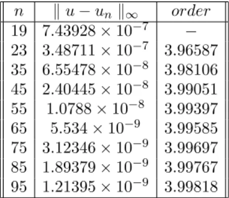
where the exact solution is u(x) = (1 +x)2. In Table 1, numerical re-sults are presented for rules Iϕ2f. We obtain an approximation to the solution of (3.4). Numerical results illustrate accuracy of the proposed quadrature rule. By increasing the value of n, the errors have been de-creased. In Table 2, we present the absolute errors of algorithm combines Trapezoidal and Simpson rules [12] for different values of n. A numeri-cal comparison between Tables 1,2 shows that spline quasi-interpolant method is more accurate than of algorithm combines Trapezoidal and Simpson rules [12].
Table 1. Max. Abs. Err. for Example 5.1 (IQ2f)
n ∥u−un∥∞ order 19 7.43928×10⁻⁷ − 23 3.48711×10⁻⁷ 3.96587 35 6.55478×10⁻⁸ 3.98106 45 2.40445×10⁻⁸ 3.99051 55 1.0788×10⁻⁸ 3.99397 65 5.534×10⁻⁹ 3.99585 75 3.12346×10⁻⁹ 3.99697 85 1.89379×10⁻⁹ 3.99767 95 1.21395×10⁻⁹ 3.99818
Example 5.2. Consider the following Volterra integral equation
u(x) + ∫ x
0
(xt2+x2t)u(t)dt=x+ 7 12x
5,
where the exact solution is u(x) =x. In Table 3, numerical results are presented for ruleIϕ2f. In table 4, we compare the absolute errors of the
Table 2. Max. Abs. Err. [12] n ∥u−un∥∞ 19 8.36×10⁻⁵ 23 4.77×10⁻⁵ 35 1.33×10⁻⁵ 45 6.29×10⁻⁶ 55 3.44×10⁻⁶ 65 2.08×10⁻⁶ 75 1.36×10⁻⁶ 85 9.35×10⁻⁷ 95 6.70×10⁻⁷
spline quasi-interpolant method for n = 32 with numerical expansion-iterative method [11]. The results show the efficiency and rate of con-vergence of the method. Figure 1 shows the maximum absolute errors for the proposed method.
Table 3. Max. Abs. Err. for Example 5.2 (IQ2f)
n ∥u−un∥∞ 20 3.88179×10⁻⁷ 40 2.42884×10⁻⁸ 60 4.79842×10⁻⁹
80 1.5183×10⁻⁹
100 6.21901×10⁻¹⁰
Example 5.3. Consider the following Volterra integral equation
u(x) +
∫ x
0
xtu(t)dt=e−x2 +x(1−e −x2
)
2 ,
where the exact solution isu(x) =e−x2.In Table 5, numerical results are presented for ruleIϕ2f. In table 6, we compare the absolute errors of the spline quasi-interpolant method for n = 32 with numerical expansion-iterative method [11]. Figure 2 shows the maximum absolute errors for the proposed method.
Table 4. Numerical results for Example 5.2 x Absolute error Absolute error[11]
0 0 1.5625×10⁻²
0.1 8.55709×10⁻⁹ 9.375×10⁻³ 0.2 1.86236×10⁻⁸ 3.125×10⁻³ 0.3 2.78283×10⁻⁸ 3.125×10⁻³ 0.4 3.36708×10⁻⁸ 9.375×10⁻³ 0.5 3.80447×10⁻⁸ 1.5625×10⁻² 0.6 4.72105×10⁻⁸ 9.375×10⁻³ 0.7 5.65627×10⁻⁸ 3.68045×10⁻³ 0.8 5.83707×10⁻⁸ 3.125×10⁻³ 0.9 4.9622×10⁻⁸ 9.375×10⁻³
50 60 70 80 90 100 n
5.´10-9
1.´10-8
1.5´10-8
2.´10-8
error
Figure 1. The absolute error∥u−un∥∞for different values of
nfor Example 5.2.
Example 5.4. Consider the following Volterra integral equation
u(x) +
∫ x
0
(x−t) cos(x−t)u(t)dt= cos(x),
where the exact solution isu(x) = 13(2 cos√3t+1).In Table 7, numerical results are presented for rule Iϕ2f. In table 8, we compare the absolute
Table 5. Max. Abs. Err. for Example 5.3 (IQ2f)
n ∥u−un∥∞ 20 4.78517×10⁻⁷ 40 3.07465×10⁻⁸ 60 6.10838×10⁻⁹ 80 1.93431×10⁻⁹ 100 7.92292×10⁻¹⁰
Table 6. Numerical results for Example 5.3 x Absolute error Absolute error[11]
0 0 3.25×10⁻⁴
0.1 7.99755×10⁻⁹ 2.02×10⁻³ 0.2 1.41309×10⁻⁸ 1.28×10⁻³ 0.3 1.37384×10⁻⁸ 1.647×10⁻³ 0.4 5.21359×10⁻⁹ 6.295×10⁻³ 0.5 8.52356×10⁻⁹ 1.2284×10⁻² 0.6 2.59421×10⁻⁸ 7.87×10⁻³ 0.7 4.61481×10⁻⁸ 2.669×10⁻³ 0.8 6.24702×10⁻⁸ 2.661×10⁻³ 0.9 6.84528×10⁻⁸ 7.562×10⁻³
errors of the spline quasi-interpolant method for n= 64 with Rational-ized Haar functions method [16]. Figure 3 shows the maximum absolute errors for the proposed method.
Table 7. Max. Abs. Err. for Example 5.4 (IQ2f)
n ∥u−un∥∞ 20 8.97969×10⁻⁷ 40 5.75157×10⁻⁸ 60 1.14124×10⁻⁸ 80 3.61664×10⁻⁹ 100 1.48246×10⁻⁹
Table 8. Numerical results for Example 5.4 x Absolute error Absolute error[16]
0 0 0.6×10⁻⁵
0.1 8.57026×10⁻⁹ 4.23×10⁻⁴ 0.2 7.42193×10⁻⁹ 3.45×10⁻⁴ 0.3 6.67605×10⁻⁹ 4.55×10⁻⁴ 0.4 6.28758×10⁻⁹ 2.7×10⁻⁵ 0.5 4.13835×10⁻⁹ 0.7×10⁻⁴ 0.6 3.59153×10⁻⁹ 3.7×10⁻⁴ 0.7 1.79297×10⁻⁹ 1.52×10⁻⁴ 0.8 2.97626×10⁻¹⁰ 6.7×10⁻⁵ 0.9 1.00404×10⁻⁹ 2.4×10⁻⁴
6. Conclusion
In this article, we illustrated a rule based on spline quasi-interpolant. In following, we employed this rule to the solution of a Volterra inte-gral equation. The numerical examples were presented to illustrate the accuracy and the implementation of the method.
50 60 70 80 90 100 n
5.´10-9
1.´10-8
1.5´10-8
2.´10-8
2.5´10-8
3.´10-8
error
Figure 2. The absolute error∥u−un∥∞for different values of
40 50 60 70 80 n 5.´10-8
1.´10-7
1.5´10-7
error
Figure 3. The absolute error∥u−un∥∞for different values of
nfor Example 5.4.
References
[1] S. Abelman, D. Eyre, A rational basis for second kind Abel integral equation, J. Comput. Appl. Math,34(1991), 281–290.
[2] M. Aigo, On the numerical approximation of Volterra integral equations of second kind using quadrature rules, International Journal of Advanced Scientific and Technical Research,1(2013).
[3] K. Atkinson, The numerical solution of integral equations of the second kind, The press Syndicate of the University of Cambridge, United Kingdom, (1997). [4] H. Brunner, The numerical solution of weakly singular Volterra integral
equa-tions by collocation on graded meshes, Math. Comput,45(1985), 417–437. [5] R.F. Cameron, S. Mckee, Product integration methods for second kind Abel
integral equations, J. Comput. Appl. Math,11(1984), 1–10.
[6] L.M. Delves, J.L. Mohamed, Computational methods for integral equations, Cambridge University Press, (1985).
[7] E.A. Galperin, E.J. Kansa, A. makroglou, S. A. Nelson, Mathematical pro-gramming methods in the numerical solution of Volterra integral and integro-differential equations with weakly singular kernel, Proceedings of the Second World Congress of Nonlinear Analysts. Athens, Greece, Nonlinear Anal. The-ory, Mehods Appl,30(1997), 1505–1513.
[8] W. Hackbusch, Integral equations theory and numerical treatment, Birkhauser, (1995).
[9] A.J. Jerri, Introduction to integral equations with applications, John Wiley and Sons, INC, (1999).
[10] Ch. Lubich, Fractional linear multistep methods for Abel-Volterra integral equa-tions of the second kind, Math. Comput,45(1985), 463–469.
[11] Z. Masouri, Numerical expansion-iterative method for solving second kind Volterra and Fredholm integral equations using block-pulse functions, Advanced Computational Techniques in Electromagnetics, (2012).
[12] A. Mennouni, A new numerical approximation for Volterra integral equations combining two quadrature rules, Applied Mathematics and Computation.218 (2011), 1962–1969.
[13] F. Mirzaee, A computational method for solving linear Volterra integral equa-tions, Appl. Math. Sci,6(2012), 807–814.
[14] M. Mustafa, Numerical solution of volterra integral equations with Delay using Block methods, AL-Fatih journal,36(2008), 42–51.
[15] M.M. Rahman, M. A. Hakim, M. Kamrul, Numerical solutions of Volterra integral equations of second kind with the help of Chebyshev polynomials, Annals of Pure and Applied Mathematics,1(2012), 158–167.
[16] M.H. Reihani, Z. Abadi, Rationalized Haar functions method for solving Fred-holm and Volterra integral equations, J. Comput. Appl. Math,200(2007), 12–20. [17] B.V. Riley, the numerical solution of Volterra integral equations with nonsmooth solutions based on sinc approximation, Appl. Numer. Math,9(1992), 249–247. [18] P. Sablonniere, A quadrature formula associated with a univariate quadratic
spline quasi-interpolant, BIT Numerical Mathematics,47(2007), 825–837. [19] P.W. Sharp, J.H. Verner, Extended explicit Bel’Tyukov pairs of orders 4 and 5
for Volterra integral equations of the second kind, Appl. Numer. Math,34(2000), 261–274.
[20] T. Tang, X. Xu, J. Cheng, On spectral methods for Volterra type integral equa-tions and the convergence analysis, J. Comp. Math,26(2008), 825–837.
Maryam Derakhshan Khanghah
Department of Mathematics, University of Mohaghegh Ardabili, P.O.Box 56199-11367, Ardabil, Iran
Email: [email protected]
Mohammad Zarebnia
Department of Mathematics, University of Mohaghegh Ardabili, P.O.Box 56199-11367, Ardabil, Iran
![Table 2. Max. Abs. Err. [12] n ∥ u − u n ∥ ∞ 19 8.36 × 10 −5 23 4.77 × 10 −5 35 1.33 × 10 −5 45 6.29 × 10 −6 55 3.44 × 10 −6 65 2.08 × 10 −6 75 1.36 × 10 −6 85 9.35 × 10 −7 95 6.70 × 10 −7](https://thumb-us.123doks.com/thumbv2/123dok_us/8380509.2226379/11.918.340.536.202.410/table-max-abs-err.webp)
![Table 4. Numerical results for Example 5.2 x Absolute error Absolute error[11]](https://thumb-us.123doks.com/thumbv2/123dok_us/8380509.2226379/12.918.248.651.188.718/table-numerical-results-example-absolute-error-absolute-error.webp)
![Table 6. Numerical results for Example 5.3 x Absolute error Absolute error[11]](https://thumb-us.123doks.com/thumbv2/123dok_us/8380509.2226379/13.918.286.598.383.605/table-numerical-results-example-absolute-error-absolute-error.webp)


