Estimation of atmospheric nutrient inputs to the Atlantic Ocean
from 50°N to 50°S based on large-scale
fi
eld sampling:
Iron and other dust-associated elements
A. R. Baker,1C. Adams,1T. G. Bell,1,2T. D. Jickells,1and L. Ganzeveld3 Received 18 December 2012; revised 8 May 2013; accepted 8 July 2013; published 18 August 2013.
[1] Atmospheric inputs of mineral dust supply iron and other trace metals to the remote
ocean and can influence the marine carbon cycle due to iron’s role as a potentially limiting micronutrient. Dust generation, transport, and deposition are highly heterogeneous, and there are very few remote marine locations where dust concentrations and chemistry (e.g., iron solubility) are routinely monitored. Here we use aerosol and rainwater samples collected during 10 large-scale research cruises to estimate the atmospheric input of iron, aluminum, and manganese to four broad regions of the Atlantic Ocean over two 3 month periods for the years 2001–2005. We estimate total inputs of these metals to our study regions to be 4.2, 17, and 0.27 Gmol in April–June and 4.9, 14, and 0.19 Gmol in September–November, respectively. Inputs were highest in regions of high rainfall (the intertropical convergence zone and South Atlantic storm track), and rainfall contributed higher proportions of total input to wetter regions. By combining input estimates for total and soluble metals for these time periods, we calculated overall percentage solubilities for each metal that account for the contributions from both wet and dry depositions and the relative contributions from different aerosol types. Calculated solubilities were in the range 2.4%–9.1% for iron, 6.1%–15% for aluminum, and 54%–73% for manganese. We discuss sources of uncertainty in our estimates and compare our results to some recent estimates of atmospheric iron input to the Atlantic.
Citation: Baker, A. R., C. Adams, T. G. Bell, T. D. Jickells, and L. Ganzeveld (2013), Estimation of atmospheric nutrient inputs to the Atlantic Ocean from 50˚N to 50˚S based on large-scale field sampling: Iron and other dust-associated elements,
Global Biogeochem. Cycles,27, 755–767, doi:10.1002/gbc.20062.
1. Introduction
[2] The atmospheric transport of mineral dust plays a
major role in the supply of nutrients such as iron (Fe) to the oceans [Jickells et al., 2005] and has a significant influence on the radiative balance of the atmosphere [Prospero and Lamb, 2003;Chiapello et al., 2005]. This transport is highly heterogeneous on a variety of spatial and temporal scales [Prospero and Lamb, 2003; Ben-Ami et al., 2009]. Heterogeneity makes the impacts of dust on climate (both direct radiative effects and indirect effects through the infl u-ence of nutrient deposition on oceanic carbon uptake) diffi -cult to assess and therefore requires the use of complex
computer models of dust uplift, transportation, and deposi-tion. These models, in turn, need to be validated with sufficient appropriate observational data to ensure that they reliably reproduce the natural dust cycle [Mahowald et al., 2005].
[3] Remote-sensing techniques, both ground-based
[Basart et al., 2009] and from satellite-borne sensors [Ben-Ami et al., 2009;Adams et al., 2012], are increasingly providing useful data on atmospheric dust transport, whereas long-term records of dust concentrations and chemical characteristics are provided by the measurements at dust collection sites. For estimating transport over the oceans, these dust collection sites are restricted to a few island or coastal locations. For instance, in the North Atlantic, records exist for sites at Barbados, Miami, Bermuda, Mace Head, and Izaña [Arimoto et al., 1995;
Prospero, 1999;Prospero and Lamb, 2003;Prospero et al., 2010], with Barbados having by far the longest and most coherent record. In the South Atlantic, however, there are no equivalent atmospheric dust records at all.
[4] Mineral dust is the dominant atmospheric source of iron
and other trace metals to the ocean. Much of the motivation for studying atmospheric dust supply to the ocean comes from the desire to better understand the role of iron inputs in the 1
Laboratory for Global Marine and Atmospheric Chemistry, School of Environmental Sciences, University of East Anglia, Norwich, UK.
2
Now at Plymouth Marine Laboratory, Plymouth, UK.
3Department of Environmental Sciences, Wageningen University and Research Centre, Wageningen, Netherlands.
Corresponding author: A. R. Baker, Laboratory for Global Marine and Atmospheric Chemistry, School of Environmental Sciences, University of East Anglia, Norwich Research Park, Norwich NR4 7TJ, UK. ([email protected])
©2013. American Geophysical Union. All Rights Reserved. 0886-6236/13/10.1002/gbc.20062
marine carbon cycle, where it is an essential nutrient for both photosynthesis and nitrogen fixation [Boyd and Ellwood, 2010]. It is well known that only a fraction of aerosol iron is soluble in seawater [Jickells et al., 2005], and it is becoming increasingly apparent that this fraction is not fixed and is likely to vary geographically [Baker et al., 2006c;Fan et al., 2006].
[5] In this work we use data obtained from aerosol and rain
sampling during a series of long transect cruises to estimate atmospheric trace metal (and hence dust) fluxes to the Atlantic Ocean. We have already used similar methods to assess annual atmospheric nitrogen inputs to the Atlantic, by coupling observations of aerosol and rainfall species concentrations to air transport and rainfall climatologies [Baker et al., 2010]. In the present study, we use our estimates of both soluble and total iron (and aluminum and manganese) atmospheric input to produce broad-scale estimates of trace metal fractional solubility over the basin. We also discuss sources of uncertainty in our estimates and compare our results to other estimates of atmospheric dust input to the Atlantic.
2. Methods
[6] As with our earlier work on N [Baker et al., 2010], our
estimates of atmospheric trace metal input to the Atlantic are based on aerosol and rain samples collected on a series of long transect cruises in the Atlantic over the period 2000– 2005. By combining chemical data for large numbers of rain (70) and aerosol (207) samples with two separate climatol-ogies, one of rainfall rate and the other of air mass transport, each covering the 5 years, 2001–2005, we scale up the observational database to provideflux estimates for various regions of the Atlantic.
[7] The estimates of atmospheric dust-associated element
inputs presented here differ in two important respects from those of our earlier work. First, we consider that neither the total number of samples collected in the northwest Atlantic nor the geographic distribution of those samples is adequate for our purposes. We therefore only report estimates of atmo-spheric inputs to four of thefive regions that we used in our N study and not for the northwest Atlantic. Second, unlike N transport [Prospero et al., 1996], mineral dust transport over the Atlantic is strongly seasonal [e.g.,Liu et al., 2008;Basart et al., 2009;Ben-Ami et al., 2009;Adams et al., 2012]. We therefore confine our dust input estimate to the seasons for which we have observational data and have modified our air transport and rainfall climatologies accordingly.
2.1. Sampling and Analysis
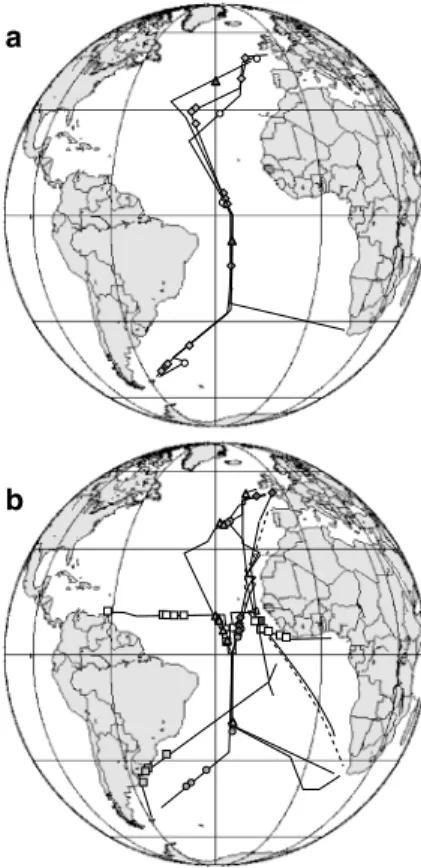
[8] Cruise tracks and aerosol sampling start locations are
shown in Figure 1. Further details of the cruises can be found in the supporting information (Table S1).
AMT12
AMT14
AMT16
M55
JCR
ANT18-1
AMT13
AMT15
ANT23-1
AMT17
Figure 1. Locations of aerosol samples used in this work for cruises which took place in (a) April–June 2003–2005 and (b) September–November 2000–2003 and (c) September– November 2004–2005. Markers show sampling start positions. Aerosol collection generally continued until the beginning of the following sample. Sampling end positions for each cruise are shown by black markers.
[9] Sampling methods for aerosol collection, including
measures taken to avoid ship-based contamination, collector flow rates, and blank collection procedures, have been de-scribed elsewhere [Baker et al., 2006b;Baker et al., 2007]. Whatman 41 collection substrates (either using Sierra-type cascade impactors with separation into coarse (>1μm diam-eter) andfine (<1μm diameter) particles, or using a single bulkfilter (see Table S1)) were used during most cruises, al-though coarse aerosol sampling during the ANT18-1 cruise was done using quartz substrates [Sarthou et al., 2003]. These had rather high blanks for total metals, and conse-quently, we do not report total metal data for that cruise. One sample during ANT18-1 (ANT18-1/A1) was collected using six cascade impactor stages, giving fractions with modal sizes of >12.5, 5, 2.4, 1.6, 0.9, 0.4, and <0.1μm. All aerosol collection substrates were washed with dilute acids before use in order to reduce trace metal blanks (see Table S2). Results of blank determinations and aerosol detection limits are reported in Tables S2 and S3.
[10] Rain samples were collected by manually opening
rain collectors (low-density polyethylene bottles attached to 28 or 40 cm diameter polypropylene funnels) immediately prior to, or at the onset of, rain and closing them upon the cessation of rain. Rain sampling equipment was cleaned prior to use by soaking in 10% vol/vol (1.58 M) HNO3for at least 48 h before use, and bottles were stored,filled with acidified (15.8 mM Aristar HNO3) ultrapure water, as described in
Baker et al. [2007]. Blanks for rain sampling were deter-mined during each cruise by collecting acidified (15.8 mM HNO3) ultrapure water that had been used to rinse the collec-tion surfaces of the rain funnels and determine the trace metal content of this rinse water (see Table S4). For three cruises (ANT18-1, JCR, and M55), subsamples of rainfall were filtered through acid-washed 47 mm 0.2μm Sartorius cellu-lose acetatefilters housed in acid-washed Milliporefiltration rigs immediately after collection, allowing us to estimate the soluble and total metal contents of these samples. All rain samples (filtered and unfiltered) for these cruises were acidified within 3 h of collection to afinal concentration of 15.8 mM with concentrated Aristar HNO3and frozen. For all other cruises, samples were frozen immediately without filtration and were subsequently acidified as above and left to stand for at least 2 weeks before analysis. Figure 2 shows the locations of the rain samples collected.
[11] Aerosol and rain samples were stored frozen and later
thawed and analyzed using methods discussed elsewhere [Baker et al., 2006a; Baker et al., 2006c; Baker et al., 2007], which for the components of interest here involve graphite furnace atomic absorption spectroscopy (GFAAS) or inductively coupled plasma-optical emission spectrometry (ICP-OES) for (soluble) Fe, Al, and Mn in rain and for soluble Fe, Al, and Mn in aerosol extracts at pH 4.7 (1.1 M ammonium acetate buffer, see Baker et al. [2007]). For JCR and M55, total aerosol Fe, Al, and Mn were determined by GFAAS/ICP-OES after digestion with concentrated HF/HNO3, as described by Baker et al. [2006c]. For the other cruises, total aerosol metals were determined by instrumental neutron activation analysis (INAA) at the Ecole Polytechnique, Montreal’s SLOWPOKE nuclear re-actor at a neutron flux of 5 × 1011cm2s1. The samples (fractions of bulk or all size fractions of segregated samples combined) were introduced in the reactor, packed
in a plastic bag, rolled into 7 mL polyethylene irradiation vials. After activation, the emission of gamma radiation at energies of 1099 (Fe-59), 1779 (Al-28), and 847 keV (Mn-55) was detected and the amount of iron, aluminum, or manganese was calculated by comparing with emissions from the standard solutions of each element. A subset of the samples that had been analyzed by the strong acid digestion method was also analyzed by INAA. This intercomparison indicated no significant differences between the two methods for Fe, Al, and Mn (pairedttest, allp<0.05,n= 11).
2.2. Wet and Dry Deposition Climatologies
[12] Here we give a brief summary of the methods used to
compile rainfall rate and air mass history climatologies, and specify differences to the climatologies used in our earlier study on N deposition [Baker et al., 2010]. Full details of the methods used can be found inBaker et al. [2010]. The principal difference to our earlier work is that here we treat only the 6 months of the year for which we have observa-tional data in constructing the climatologies. As mentioned above, we do not report atmospheric input estimates for the northwest Atlantic here, although we do give whatever information we have for that region where possible.
a
b
Figure 2. Locations of rainfall samples collected during this work for cruises which took place in (a) April–June and (b) September–November. Shapes indicate cruises which took place in 2000–2002 (squares), 2003 (circles), 2004 (diamonds), and 2005 (triangles), with solid symbols corresponding to those used for aerosol sampling locations in Figure 1. Rainfall was not collected during cruise ANT23-1 (dashed line).
[13] For the wet deposition climatology, we calculated
average precipitation rates for the two“seasons”April–June (AMJ) and September–November (SON) for which we have rainwater concentration data. Precipitation rates were obtained from the 2.5 × 2.5° gridded monthly output of the CMAP model updated from Xie and Arkin [1997] (http:// www.cdc.noaa.gov/cdc/data.cmap.html). Using that data, we calculated average precipitation rates (P) for five broad regions having relatively high (intertropical convergence zone (ITCZ; R3) and North and South Atlantic storm tracks (R1 and R5)) and low (North and South Atlantic dry regions (R2 and R4)) rainfall (Figure 3). Average precipitation rates varied from 0.6 mm d1in Region 4 in SON to 4.9 mm d1 in Region 3 in AMJ. For each of those regions, we calculated volume-weighted-mean (VWM) rainfall trace metal concen-trations from the compositions of the individual rain samples (equation (1)) and then wet depositionflux (equation (2)) for each species in the AMJ and SON periods.
CR¼∑ CiVi
∑Vi
(1) whereCiis the measured concentration andVithe volume of rain collected for each sample. The use of individual sample volumes here introduces some uncertainty into this calcula-tion, because quantitative recovery of precipitation is very difficult aboard ship, generally being underestimated. The impact of this under-sampling on measured and calculated concentrations (Ci andCR) is not easily estimated because
concentration typically varies with the duration of the precip-itation event.
Fw¼C
RP (2)
[14] For the calculation of soluble trace metal wet
deposi-tionfluxes, we did not have filtered rain samples for many of the cruises (see above). In those cases, we estimated solu-ble trace metal concentrations from total concentrations using median values for the fraction of total concentration that passed through a 0.2 or 0.45μmfilter, using our own data (Fe data from Sarthou et al. [2003] and Baker et al. [2007], and unpublished Al and Mn data for the same samples) and values reported by Prospero et al. [1987],
Lim et al. [1994] (for Al), and Buck et al. [2010] (for Fe and Al). These data are summarized in Figure 4. This opera-tional definition of soluble trace metal fraction will inevitably include a contribution from colloidal, as well as truly dissolved, material.
[15] Our dry deposition climatology is based on the
obser-vation that for many species, aerosol concentrations over the ocean are related to the source regions that an air mass has had contact with in the recent past [e.g., Baker et al., 2006b]. Here we use the same source regions as in our earlier work on nitrogen deposition [Baker et al., 2010], namely North America (NAmer), Europe (Eur), North Africa (Sahara), Southern Africa (SAfr), Southern Africa influenced by biomass-burning emissions (SAfr-BB), South America (SAmer), and remote air that had been circulating over the ocean (in either hemisphere) for 5 days prior to collection (NAtl-Rem and SAtl-Rem). The inclusion of a separate SAfr-BB source is justified for nitrogen because biomass
2a
3a1
4a 5a
2b
2c 2d
3a2 3b
4b 4c
4d 5b
1a
1b
1c 1d
1e
Figure 3. Map showing the boundaries (solid lines) of the deposition regions used in this study. Labels (2a–5b) identify dry deposition subregions (dashed lines), with points showing locations at which air mass back trajectories were obtained for the determination of the air mass climatology.
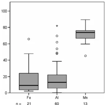
Figure 4. Box and whisker plots showing the percentage of soluble Fe, Al, and Mn in rain samples collected over the Atlantic Ocean. Also shown is the number of observations (n) in each category. Outliers more than 1.5 times the interquartile range are indicated by circles and extremes greater than three times the interquartile range by stars.
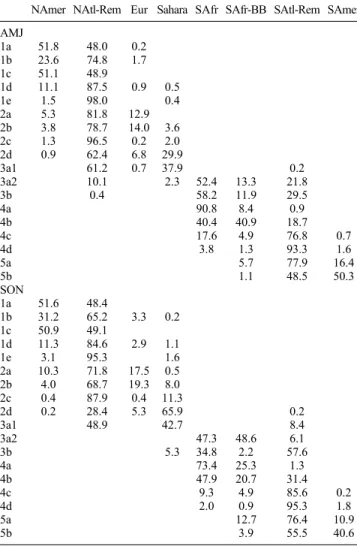
burning is a significant source of both reduced and oxidized nitrogen [Andreae and Merlet, 2001]. We include this source specifically here because biomass burning has been suggested to be a potentially significant source of soluble Fe [Guieu et al., 2005;Luo et al., 2008]. Samples influenced by biomass burning were identified using nonseasalt potassium as a tracer [Baker et al., 2006b;Baker et al., 2010]. In order to assess the contribution of each source region to air flow over the Atlantic, we subdivided the wet deposition regions discussed above into smaller subregions (Figure 3). We then obtained 5 day air mass back trajectories for points within each subregion using ECMWF archive data from the British Atmospheric Data Centre (http://badc.nerc.ac.uk/community/trajectory/) for each day of the 5 year period and classified them according to which source region they had passed over. The criteria used to make this classification were identical to those we used in our earlier work [Baker et al., 2010]. Table 1 shows the fractional occur-rence of each air mass type (wi) at each climatology point for the AMJ and SON periods.
[16] Aerosol samples were also classified according to the
same criteria using 5 day air mass back trajectories obtained from the NOAA Hybrid Single-Particle Lagrangian Integrated Trajectory model (FNL data set). In each of the five large
regions in each season, we calculated the median aerosol con-centrations (CAi) for each air mass type and these median values were assumed to be representative of the aerosol concentrations associated with that air mass type in each region. Dry deposition fluxes were then calculated from these concentrations using aerosol particle size- and wind speed-dependent dry deposition velocities (vd) for fine and coarse aerosols, as described in
Baker et al. [2010]. We calculated dry deposition velocities for each subregion and time period using the method of
Ganzeveld et al. [1998], utilizing climatological mean wind speeds for the relevant months of 2001–2005 obtained from the ECMWF ERA-Interim data set and particle sizes of 0.6μm for submicron particles and 5μm for supermicron parti-cles. These values were derived from mass median diameters calculated for soluble Fe for the seven size fractions of sample ANT18-1/A1 (see above). The calculated deposition velocities fall in the range 0.02–0.03 and 0.4–1.1 cm s1 for fine and coarse modes, respectively. Each air mass’contribution to the total deposition in each subregion was weighted according to its fractional contribution to the total air flow there (wi, Table 1), as derived from the air mass classification scheme (equation (3)):
Fd;int¼∑wiCcA;ivcdþCfA;ivfd (3) [17] For the AMT16 and ANT23-1 cruises for soluble metals
and for most cruises for total metals, we only collected bulk (i.e., non-size fractionated) aerosol concentrations. In those cases, we artificially split these values into fine and coarse components using median fractions of each species occurring in the coarse mode derived from our size-fractionated data (see Table S5) as done previously [Baker et al., 2010].
3. Results
[18] Below we summarize atmospheric trace metal
concen-trations and depositionfluxes obtained in our study.
3.1. Wet Deposition—Rainfall Chemical Characteristics and Deposition Fluxes
[19] In Table 2, we show concentrations of total rainwater
Fe, Al, and Mn for each deposition region in the AMJ and
Table 1. Percentage Occurrence of Different Air Mass Types (wiam) at Selected Points in the Atlantic, Based on Analysis of Daily 5 Day Air Mass Back Trajectories for the Months of April–June (AMJ) and September–November (SON) in the Years 2001–2005
NAmer NAtl-Rem Eur Sahara SAfr SAfr-BB SAtl-Rem SAmer AMJ
1a 51.8 48.0 0.2 1b 23.6 74.8 1.7 1c 51.1 48.9
1d 11.1 87.5 0.9 0.5
1e 1.5 98.0 0.4
2a 5.3 81.8 12.9 2b 3.8 78.7 14.0 3.6 2c 1.3 96.5 0.2 2.0 2d 0.9 62.4 6.8 29.9
3a1 61.2 0.7 37.9 0.2
3a2 10.1 2.3 52.4 13.3 21.8
3b 0.4 58.2 11.9 29.5
4a 90.8 8.4 0.9
4b 40.4 40.9 18.7
4c 17.6 4.9 76.8 0.7
4d 3.8 1.3 93.3 1.6
5a 5.7 77.9 16.4
5b 1.1 48.5 50.3
SON
1a 51.6 48.4
1b 31.2 65.2 3.3 0.2 1c 50.9 49.1
1d 11.3 84.6 2.9 1.1
1e 3.1 95.3 1.6
2a 10.3 71.8 17.5 0.5 2b 4.0 68.7 19.3 8.0 2c 0.4 87.9 0.4 11.3
2d 0.2 28.4 5.3 65.9 0.2
3a1 48.9 42.7 8.4
3a2 47.3 48.6 6.1
3b 5.3 34.8 2.2 57.6
4a 73.4 25.3 1.3
4b 47.9 20.7 31.4
4c 9.3 4.9 85.6 0.2
4d 2.0 0.9 95.3 1.8
5a 12.7 76.4 10.9
5b 3.9 55.5 40.6
Table 2. Concentration Ranges (nmol L1) and Number of Samples (in Parentheses) for Total Fe, Al, and Mn, and Their Volume-Weighted-Mean Concentrations (CR) for the Rain Samples Collected in Each of the Wet Deposition Regions During the Periods April– June (AMJ) and September–November (SON)
Region Fe CR
Fe
Al CR Al
Mn CR Mn
AMJ
NAtl Storm 117–534 (3) 229 86–1750 (3) 404 14–76 (3) 28 NAtl Dry 367 (1) 367 1070, 1290 (2) 1130 32, 71 (2) 42 ITCZ 20–716 (7) 213 15–1160 (7) 462 1.1–44 (7) 15 SAtl Dry 42,<176 (2) 58 118, 287 (2) 138 4.0, 18 (2) 5.6 SAtl Storm 189, 724 (2) 228 197–4290 (4) 2080 <6.4–49 (4) 31
All 204 683 19
SON
NAtl. Storm 110–2240 (4) 680 165–4760 (4) 1470 6.2–77 (4) 28 NAtl. Dry 40–637 (5) 82 25–2160 (5) 182 0.9–60 (5) 5.9 ITCZ 33–2050 (33) 515 40–6930 (35) 1350<0.5–153 (31) 25 SAtl Dry 35–105 (5) 70 <27–424 (5) 140 4.0–24 (5) 17 SAtl Storm <30–1440 (5) 338 97–5420 (5) 701 2.6–28.3 (5) 10
SON seasons, and volume-weighted-mean concentrations for each region and for the Atlantic as a whole in each season. Overall, the concentrations of rainwater trace metals ranged from 20 to 2240, 15–6930, and<0.5–153 nmol L1for Fe, Al, and Mn, respectively. VWM concentrations for each spe-cies were higher in SON than in AMJ (e.g., for Fe, the VWM concentrations for all samples were 204 nmol L1 in AMJ and 493 nmol L1in SON), although some caution may be necessary in interpreting this difference because of the low number of samples available for AMJ (~15, compared to ~50 in SON). Our data are in reasonable agreement with previously published rainwater trace metal concentrations (Table 3), although in several of our deposition regions, and for Mn in general, there is very little other data available. [20] In Table 4, we show our calculated wet deposition
fluxes for total metals in Regions 2–5. Fluxes were lowest in Region 4 for all metals, as a result of low rainfall concen-trations and precipitation rates, and highest in Region 3, where both concentrations and precipitation were high. As stated above, we used median values of percentage of soluble rainwater trace metals (9.4%, 13%, and 74% for Fe, Al, and Mn, respectively) to calculate soluble metal concentrations for most of our rain samples. Soluble metal wet deposition fluxes (Table 4) were of similar percentages with their re-spective total wetfluxes, since most of the soluble metal data were calculated in this way, rather than measured directly.
3.2. Dry Deposition—Chemical Characteristics of Air Mass Types and Deposition Fluxes
[21] In Tables 5 and 6, we show median aerosol trace metal
concentrations for each air mass type observed in each of the five deposition regions during the AMJ and SON periods, respectively. We also present the variation in aerosol trace metal concentrations between air mass types (without dividing the data set according to deposition region) for these two periods in Figure 5.
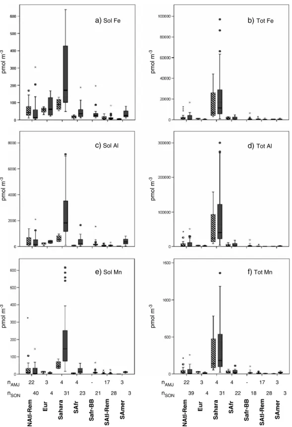
[22] Trace metal concentrations were generally higher in
Regions 1–3 than in Regions 4 and 5, consistent with the distributions of their terrestrial sources between the hemi-spheres. As might be expected, aerosol trace metal concen-trations were very much higher in Saharan air masses than in any other air mass type. For the total metals, no air mass type had a median concentration greater than 10% of its re-spective median concentration in Saharan air. For the soluble metals, however, the median concentrations of the non-Saharan air masses were of higher proportions than the
Table 3. Examples of Previously Reported Concentrations (nmol L1) and Number of Observations (Where Available) for Total Iron, Aluminum, and Manganese in Rainfall Samples in Each of the Five Deposition Regions Used in This Work
Region Month Fe Al Mn n Referencesa
1 Aug 314b 12 A
1 Mar 225b 4 A
2c 0.9–495 4.8–431 0.5–7.3 12 B
2c Jun 25.6 103 1 C
3 Oct/Nov 150–1140 330–4860 8.3–62 3 D
3 Jun 54–3300 (680b) 1.6–160 (31.0b) 17 E
3 Jul 132–419 414–1404 4 C
4 May/Jun 3.6, 16 2 E
5 Nov 30, 62 48, 380 2.0, 3.8 2 D
5 May 121 2.0 1 E
a
References: A,Kieber et al. [2003]; B,Lim et al. [1991]; C,Buck et al. [2010]; D,Helmers and Schrems[1995]; E,Kim and Church[2002]. bVolume-weighted-mean concentration.
c
North of Region 2.
Table 4. Precipitation Rate (P, mm d1) and Wet Deposition Fluxes (nmol m2d1) of Soluble and Total Fe, Al, and Mn to Deposition Regions for the Periods April–June (AMJ) and September–November (SON)
Region P Sol Fe Sol Al Sol Mn Tot Fe Tot Al Tot Mn AMJ
1 2.7 - - -
-2 0.7 24.6 104 22.2 260 800 30
3 4.9 97.4 292 52.1 1040 2250 71
4 1.0 5.4 17.7 4.1 58 140 5.5
5 3.5 74.2 937 80.5 790 7210 110
SON
1 3.8 - - -
-2 2.2 16.8 51.3 9.4 180 390 13
3 4.2 114 612 66.2 2180 5690 110
4 0.6 3.9 10.7 7.3 41 82 9.9
5 3.3 231 393 27.3 1100 2300 34
Table 5. Median Concentrations (pmol m3) and Number of Observations (n) for Soluble and Total Metals for the Aerosol Samples Collected During the Period April–June (AMJ) Divided According to Air Mass Type in Each of the Five Deposition Regions
Region Air Mass Sol Fe Sol Al Sol MnnSolTot Fe Tot Al Tot MnnTot
1 NAmer - - -
-NAtl-Rem 41.6 248 7.9 5 1210 1590 15.8 5
Eur - - -
-Sahara - - -
-2 NAmer - - -
-NAtl-Rem 33.5 132 9.1 14 1260 1850 19.6 14 Eur 58.9 286 15.2 3 1280 3070 30.9 3
Sahara - - -
-3 NAtl-Rem 77.3 717 32.0 3 3420 10,800 56.4 3
Eur - - -
-Sahara 88.9 552 45.1 4 6820 24,300 139 4 SAfr 8.8 58.4 4.2 2 1700 6350 38.3 2
SAfr-BB - - -
-SAtl-Rem 34.4 228 11.0 1 1460 4220 27.3 1 4 SAfr 24.4 94.2 5.9 2 1580 1880 16.4 2
SAfr-BB - - -
-SAtl-Rem 10.7 58.4 1.9 11 363 523 7.0 11
SAmer - - -
-5 SAfr-BB - - -
-SAtl-Rem 4.6 70.9 1.5 5 379 729 4.6 5 SAmer 4.1 32.1 0.6 3 565 788 2.6 3
Saharan median concentrations (e.g., up to 37% (Eur), 19% (Eur), and 11% (SAfr) for soluble Fe, Al, and Mn respec-tively). A few samples in the NAtl-Rem classification had high trace metal concentrations (Figure 5). The color of these samples, which were generally located in the west of Region 3, indicated that they contained significant amounts of Saharan dust, although their air mass back trajectories did not show contact with land over the 5 days before collection. [23] Figure 5 appears to show that trace metal
concentra-tions in Saharan air were both higher and more variable in SON than in AMJ. This may not actually be the case. The for-mer is probably the result of the AMJ cruises all passing through the central Atlantic, while several of the SON cruises approached much closer to the West African coast (Figure 1) and hence encountered higher dust concentrations. The ap-parent lower variability of AMJ concentrations may also be partly due to the uniformity of the AMJ cruise tracks through the tropical North Atlantic and may also simply be a result of the lower number of samples collected over that period (four in AMJ, 31 in SON).
[24] Our median trace metal concentration data (Tables 5
and 6) and their ranges (Figure 5) are consistent with previ-ous ship-board studies in the Atlantic, although there is a high degree of variability in observed trace metal concentra-tions in all of these data. For example, total and soluble Fe concentrations have been reported in the range 1.4– 134,000 pmol m3[Völkening and Heumann, 1990;Losno
et al., 1992;Rädlein and Heumann, 1992, 1995;Johansen et al., 2000; Chen and Siefert, 2004; Baker et al., 2006c;
Buck et al., 2010] and <2.0–775 pmol m3 [Johansen et al., 2000; Chen and Siefert, 2004; Baker et al., 2006c;
Buck et al., 2010], respectively. In Tables S6 and S7, we list examples of, respectively, total and soluble aerosol trace metal concentrations previously reported for ourfive deposi-tion regions. While we have not attempted to select for data in these periods, it would appear that most previous studies have taken place in the same seasons as ours.
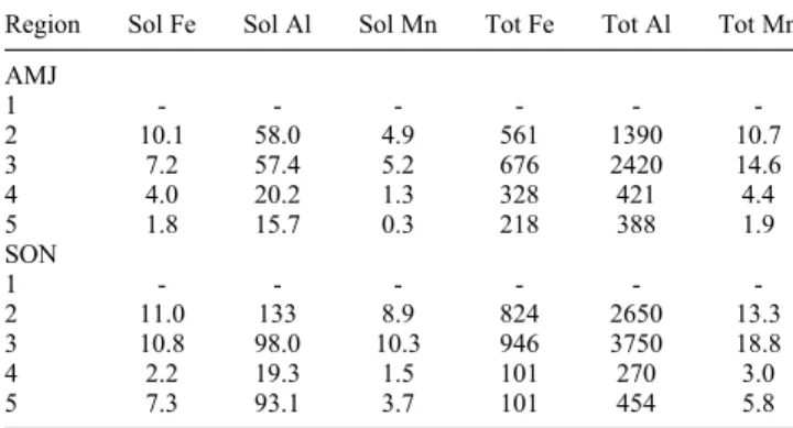
[25] Similarly to wet deposition, dry deposition fluxes
were generally low in Region 4 in both seasons (Table 7), although the lowest dry deposition fluxes (for all species except total Fe and total Al) were recorded in Region 5 in AMJ. The highest dry deposition fluxes in both seasons occurred in Region 3 for total metals and Region 2 for soluble metals.
3.3. Total Trace Metal Inputs and Climatological Mean Solubility
[26] In Table 8, we show the total combined wet and dry
inputs of trace metals to the deposition regions over each of the 3 month periods considered. For each trace metal species, inputs were lowest in Region 4 in both seasons and inputs to the high-precipitation regions (3 and 5) were generally higher than those in Regions 2 and 4 by factors of at least 2. In the high-precipitation regions, wet deposition constituted a higher proportion of the total input than in the drier regions (Figure 6 and Table S12). In almost all cases, the propor-tion of soluble trace metals delivered via rainfall was higher than the equivalent proportion of total trace metals (Figure 6), because the fractional solubility of rainwater trace metals is higher than their fractional solubility in aerosol.
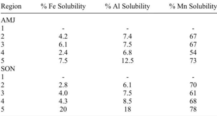
[27] We used the inputs of soluble and total Fe, Al, and Mn
presented in Table 8 to calculate overall climatological mean solubilities for each metal (% solubility = 100 × soluble in-put / total inin-put). The results of these calculations are given in Table 9 and lie in the range 2.4%–20%, 6.1%–18%, and 54%–78% for Fe, Al, and Mn respectively.
4. Discussion
4.1. Sources of Uncertainty in Our Flux Estimates
[28] There are many potential sources of uncertainty in the
trace metalflux estimates that we present here. Some of these uncertainties are common to our earlier estimate of nitrogen
Table 6. Median Concentrations (pmol m3) and Number of Observations (n) for Soluble and Total Metals for the Aerosol Samples Collected During the Period September–November (SON) Divided According to Air Mass Type in Each of the Five Deposition Regions
Region Air Mass Sol Fe Sol Al Sol Mn nSol Tot Fe Tot Al Tot Mn nTot
1 NAmer - - -
-NAtl-Rem 17.4 227 2.0 6 384 534 2.0 6
Eur - - -
-Sahara - - -
-2 NAmer - - -
-NAtl-Rem 11.2 90.0 3.2 28 349 594 6.5 28
Eur 61.7 367 4.5 4 240 1220 7.8 4
Sahara 158 1820 115 17 11,500 36,700 167 15
SAtl-Rem - - -
-3 NAtl-Rem 82.2 702 53.4 6 5290 21,500 93.2 5
Sahara 229 2050 159 14 19,200 79,000 341 14
SAfr 40.3 273 18.5 22 864 2630 17.4 20
SAfr-BB 37.7 142 9.0 8 730 1940 17.8 7
SAtl-Rem - - -
-4 SAfr 13.5 48.5 5.2 3 198 1120 11.8 2
SAfr-BB 19.7 137 9.0 13 515 1520 15.7 11
SAtl-Rem 6.4 56.5 1.5 20 376 491 3.5 20
SAmer - - -
-5 SAfr-BB - - -
-SAtl-Rem 19.2 84.3 4.0 8 167 458 8.7 8
a) Sol Fe
NAtl-Rem
Eur
Sahara
SAfr
Safr-BB
SAtl-Rem
SAmer
pmol m
-3
pmol m
-3
pmol m
-3
NAtl-Rem
Eur
Sahara
SAfr
Safr-BB
SAtl-Rem
SAmer
c) Sol Al
e) Sol Mn
b) Tot Fe
d) Tot Al
f) Tot Mn
Figure 5. Box and whisker plots showing total (coarse +fine) concentrations of (a) soluble and (b) total Fe, (c) soluble and (d) total Al, (e) soluble and (f) total Mn according to air mass type for the periods April–June (hatched boxes) and September–November (grey boxes). Figures 5a–5f show the number of observations (n) in each category. Air mass types are defined in the text. Outliers and extremes are indicated as in Figure 4.
deposition to the Atlantic and were discussed in detail there [Baker et al., 2010]. We identify those uncertainties below but only give specific analysis of the uncertainties peculiar to the trace metal estimate here. Where sources of uncertainty are common to the various trace metal estimates, we illustrate their impact, taking Fe as an example and only list uncer-tainties for metals individually where those unceruncer-tainties are metal specific, e.g., for wet inputs of soluble trace metals.
4.1.1. Wet and Dry Deposition Flux Parameterizations
[29] Rainfall rates are uncertain due to difficulties of
making reliable measurements over the ocean, but this probably is not a large contributor on the broad spatial scales considered in this work [Baker et al., 2010].
[30] Dry deposition velocity (vd) remains a major uncer-tainty in estimating atmosphericfluxes to the ocean. Duce et al. [1991] used a vdvalue of 0.4 cm s1for bulk aerosol to estimate the dry deposition of mineral dust to the oceans. They also suggested thatvdvalues of 0.01 and 1 cm s1might be appropriate for fine mode (<1μm) and mineral dust aerosols, respectively. Using thesevdvalues in our deposi-tion estimate, we calculate the cumulative dry input of total Fe to Regions 2–5 in SON to be 2.3 Gmol (vd= 0.4 cm s1) and 3.8 Gmol (vd= 0.01 and 1 cm s1), compared to the value of 1.9 Gmol derived using the variable deposition velocities of our baseline calculation. While there is a factor of 2 differ-ence between these deposition estimates, this is well within the uncertainty in dry deposition velocity (plus or minus a factor of 2–3) quoted byDuce et al. [1991] and associated with uncertainties on the role of, for example, the impact of spray formation and hygroscopic growth on aerosol deposi-tion [Ganzeveld et al., 1998;Petroff and Zhang, 2010]. As an indication of the potential impact of this uncertainty, increasing dry deposition velocities by a factor of three increases the (dry plus wet) input of total Fe, Al, and Mn to Regions 2–5 combined by 69%, 89%, and 40%, respectively in SON.
4.1.2. Volume-Weighted-Mean Rainwater Concentrations
[31] Our wet deposition estimates are based on the
assump-tion that the volume-weighted-mean species concentraassump-tions used in the calculations are actually representative of the rainfall in each region. Two factors are likely to affect the validity of this assumption: (i) whether the number of sam-ples we collected was sufficient to characterize rainwater composition in each region and (ii) whether the geographic
distribution of those samples was representative of the re-gion. In the former case, we do not have sufficient other data to compare against rainwater trace metals, so we use our previous estimates for N to assess likely uncertainties. Thus, we assign uncertainties of ±20% in VWM concentra-tions in Region 3 in SON (for which we had more than 30 samples) and ±40% for all other regions (where we had fewer than 10 samples). This implies an overall uncertainty in our estimate of total wet input to Regions 2–5 of ±40% in AMJ and ±27% in SON. In the latter case, the distribution of our rain samples is poor in all regions (except perhaps Region 3 in SON) due to the constraints of the cruise tracks used in this study (Figure 2). We are not able to quantify the uncertainty associated with this poor sample distribution without further information on rainwater trace metal concentrations over the Atlantic. This may be a significant effect where relatively large mineral dust inputs occur (e.g., for the Sahara in Regions 2 and 3 and the Namib desert in Region 4), since these are likely to be strongest at the margins of our regions. [32] Ridame and Guieu [2002] noted that very small
(i.e., only a few drops) rainfall events can contribute signif-icant amounts of dust to the western Mediterranean. Events of this type are rather difficult to sample, particularly from ships, and if a similar situation exists in the eastern North Atlantic (Region 2), our sampling would be unlikely to record them.
[33] The soluble metal wet depositionflux estimates given
in Table 4 are subject to further uncertainty because of the way in which we have estimated trace metal soluble fractions in samples for which we had no soluble metal measurements. Fractional Fe and Al solubility in rainfall varies as a function of pH [Prospero et al., 1987;Theodosi et al., 2010a] and total metal load [Theodosi et al., 2010a]. Since we do not have rainwater pH data available and are not able to estimate metal loadings as part of our calculations, we estimate the uncer-tainty in soluble trace metal wet depositionfluxes using the interquartile ranges of the fractional solubility data presented in Figure 4. This approach yields ranges of wet soluble inputs of 0.33–0.63, 0.8–1.5, and 0.109–0.116 Gmol for Fe, Al, and Mn respectively in SON, compared to our baseline estimates for these species of 0.41 Gmol (Sol Fe), 1.1 Gmol (Sol Al), and 0.115 Gmol (Sol Mn).
4.1.3. Median Aerosol Concentrations
[34] As for N [Baker et al., 2010], we estimate the
uncer-tainty due to poor characterization of representative aerosol
Table 7. Dry Deposition Fluxes (nmol m2d1) of Soluble and Total Metals to Deposition Regions for the Periods April–June (AMJ) and September–November (SON)
Region Sol Fe Sol Al Sol Mn Tot Fe Tot Al Tot Mn AMJ
1 - - -
-2 10.1 58.0 4.9 561 1390 10.7
3 7.2 57.4 5.2 676 2420 14.6
4 4.0 20.2 1.3 328 421 4.4
5 1.8 15.7 0.3 218 388 1.9
SON
1 - - -
-2 11.0 133 8.9 824 2650 13.3
3 10.8 98.0 10.3 946 3750 18.8
4 2.2 19.3 1.5 101 270 3.0
5 7.3 93.1 3.7 101 454 5.8
Table 8. Total (Wet + Dry) Inputs (Gmol) of Soluble and Total Fe, Al, and Mn to Deposition Regions for the Periods April–June (AMJ) and September–November (SON)
Region Sol Fe Sol Al Sol Mn Tot Fe Tot Al Tot Mn AMJ
1 - - -
-2 0.032 0.15 0.025 0.76 2.01 0.037
3 0.097 0.33 0.053 1.60 4.35 0.079
4 0.014 0.056 0.008 0.57 0.82 0.015
5 0.093 1.17 0.010 1.24 9.34 0.136
SON
1 - - -
-2 0.025 0.17 0.017 0.92 2.79 0.024
3 0.116 0.66 0.071 2.91 8.79 0.116
4 0.009 0.044 0.013 0.21 0.52 0.019
concentrations, based on the number of samples (n) used to calculate the median concentrations for each air mass type. Thus, we assigned uncertainties of ±100%, wherenwas≤2, ±50% for 3<n≤5, ±30% for 6<n≤10, and ±15% for
n>10. This resulted in uncertainties in dry input to the indi-vidual regions of 27%–70% in AMJ and 19%–39% in SON for soluble Fe, and 31%–86% (AMJ) and 15%–36% (SON) for total Fe. Overall uncertainties for dry inputs to Regions 2–5 combined were 50% (AMJ) and 25% (SON) for soluble Fe, and 60% (AMJ) and 21% (SON) for total Fe. As was the case for wet inputs, the geographic distribution of aerosol samples through each region is likely to affect our calculated median trace metal concentrations. We are not able to quantify the impact of this effect.
4.1.4. Wet and Dry Soluble Metal Inputs
[35] We have used somewhat different operational defi
ni-tions to define the soluble fractions of the rainfall and aerosol samples in this study. In both cases, we filtered samples through 0.2μmfilters, which will lead to our“soluble” frac-tions containing trace metals that would more accurately be defined as “dissolved and colloidal”. The pH of the rain and aerosol systems was also different. We buffered the aerosol extraction experiments at pH 4.7 but made no attempt to buffer the rain samples at afixed value beforefiltration, nor did we measure the pH of any but a handful of the rain samples. Reports of rainwater pH in the remote Atlantic give values in the range 4.19–5.73 [Losno et al., 1991;Lim et al., 1994]. The samples collected in the ITCZ had higher pH values (median 5.36) than those from other regions (median 4.67), probably due to partial neutralization of acidity by CaCO3 in Saharan dust in the ITCZ samples [Loye-Pilot
et al., 1986]. Since trace metal solubility decreases with
increasing pH [Theodosi et al., 2010a; Theodosi et al., 2010b], this might imply that our results overestimate the importance of dry deposition to atmospheric soluble trace metalfluxes in Region 3.
4.2. Contributions of Saharan Dust and Other Sources
[36] Our calculations allow us to assess the contributions
of individual air mass types to total dry atmospheric inputs to our study region. Concentrations of soluble and total Fe, Al, and Mn were significantly higher in air masses dominated by Saharan dust than in aerosols sampled in any other air mass type (Figure 5). According to our climatological esti-mates for dry deposition, Saharan dust inputs to Regions 2 and 3 contribute 17% of atmospheric soluble Fe and 21% of total Fe input to Regions 2–5 in AMJ and 38% of soluble Fe and 68% of total Fe in SON. In both seasons, the contribu-tion of Saharan dust to soluble Fe is lower than the total Fe. This is consistent with the relatively low fractional solubility of Fe in Saharan dust compared to aerosols collected from other sources reported by many workers [e.g.,Baker et al., 2006c; Sedwick et al., 2007]. The percentage contribution values from Saharan dust in AMJ are surprisingly low, perhaps (as discussed above) due to the influence of the geographic distribution of the AMJ cruises on the median aerosol concentrations we used.
[37] Observations in the Mediterranean prompted Guieu et al. [2005] to suggest that biomass burning might be a significant source of aerosol soluble Fe to the oceans. We use our results for soluble Fe in aerosols originating from southern Africa to assess whether biomass burning might be important in the South Atlantic. The median concentration of soluble Fe in aerosol samples collected from SAfr-BB-type air masses during SON (which overlaps with the south-ern hemisphere biomass-burning season) was 26 pmol m3 (n= 23) compared to 35 pmol m3(n= 25) in SAfr-type aero-sols in the same season. These two air mass types contribute 8% (SAfr-BB) and 14% (SAfr) of the soluble Fe input to Regions 2–5 in SON according to our climatology. Thus, our results do not indicate that biomass burning is a major contributor to soluble Fe inputs to the South Atlantic.
4.3. Trace Metal Solubility
[38] Percentage solubility values (100 × soluble
concentra-tion / total concentraconcentra-tion) for the individual aerosol samples collected during this study are in the range 0.1%–98% for b) Total Metals -AMJ
0 10 20 30 40 50 60 70 80 90 100
a) Soluble Metals -AMJ
d) Total Metals -SON
2 3 4
Region c) Soluble Metals -SON
% Wet
5 0
10 20 30 40 50 60 70 80 90 100
% Wet
0 10 20 30 40 50 60 70 80 90 100
2 3 4
Region
% Wet
5 0
10 20 30 40 50 60 70 80 90 100
% Wet
Figure 6. The percentage of total inputs to the deposition regions due to wet deposition for (a) soluble metals in AMJ, (b) total metals in AMJ, (c) soluble metals in SON, and (d) total metals in SON. Fe (grey bars), Al (white bars), and Mn (black bars).
Table 9. Average Percentage Solubilities Estimated From Climatological Atmospheric Inputs of Soluble and Total Trace Metals in AMJ and SON
Region % Fe Solubility % Al Solubility % Mn Solubility AMJ
1 - -
-2 4.2 7.4 67
3 6.1 7.5 67
4 2.4 6.8 54
5 7.5 12.5 73
SON
1 - -
-2 2.8 6.1 70
3 4.0 7.5 61
4 4.3 8.5 68
Fe [Sholkovitz et al., 2012], 0.2%–87% for Al, and 4.5%– 96% for Mn, with median values of 2.5%, 8.0%, and 50%, respectively (similar relative solubility patterns are also ap-parent in rainfall samples for these metals (see Figure 4 and Table 4).) For Saharan dust samples, Fe and Al solubilities lie at the lower end of these ranges (<5% and<10%, respec-tively), while aerosols from other air mass types had higher solubilities for these metals [Baker et al., 2006c]. For Fe, more soluble anthropogenic sources of Fe may contribute to the high percentage solubility of non-Saharan aerosols [Sedwick et al., 2007;Sholkovitz et al., 2012], but it is unclear whether Al solubility is also influenced by anthropogenic sources.
[39] In contrast, the percentage solubility values for Fe, Al,
and Mn shown in Table 9 represent averages of the solubil-ities for each metal, taking into account inputs of total and soluble species in both dry and wet depositions and the cu-mulative contribution from all aerosol sources to each region over the 3 month periods of our study. As such, they are more representative of trace metal solubility over timescales relevant to the residence time of these species in surface seawater [Jickells et al., 1994; de Jong et al., 2007] than the measurements of solubility made on individual aerosol or rain samples. For Fe, seawater composition strongly infl u-ences the dissolution of atmospherically deposited material [Baker and Croot, 2010]. Therefore, in Regions 2 and 3, the actual percentage of atmospheric Fe dissolved in surface waters may be rather less than the values given in Table 9
because of the high dissolved Fe concentration of the tropical North Atlantic [Sarthou et al., 2003;Measures et al., 2008]. [40] In Figure 7, we plot our estimates of total Fe and total
Mn inputs via wet plus dry (Table 8) and dry (Table S10) de-positions against total Al input. Ratios of Fe:Al in dry plus wet and dry depositions and of Mn:Al in dry deposition are generally similar to the ratios of these elements in shale [Turekian and Wedepohl, 1961]. For Mn:Al, in wet plus dry deposition, however, there is a noticeable displacement from the shale ratio, which indicates that Mn is preferentially removed during wet deposition. We suggest that this behav-ior may be caused by the much higher solubility of Mn rela-tive to Al and Fe noted above. Mn-containing (or Mn-coated) particles are likely to be more hydrophilic than Fe/Al-containing particles and therefore more likely to be incorpo-rated into cloud droplet and subsequently rained out.
4.4. Comparison to Other Flux Estimates
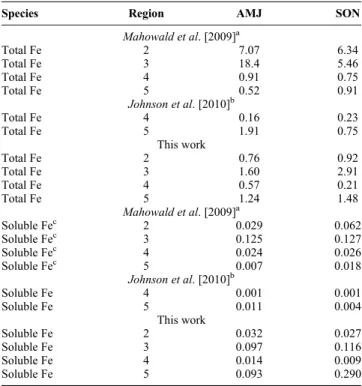
[41] In Table 10, we compare our estimates of total and
sol-uble Fe inputs to those produced by two recent modeling studies of atmospheric Fe deposition. Mahowald et al. [2009] estimated global total Fe inputs from modeled mineral dust deposition by assuming that Fe constitutes 3.5% of dust and soluble Fe inputs by assuming that reaction with atmospheric acids increases the solubility of hematite in dust from a baseline of 0.4% and that there is an additional source of Fe from combustion processes (4% of which is soluble).
Johnson et al. [2010] modeled mineral dust inputs to the South Atlantic and calculated soluble Fe inputs from these, assuming 3.5% of dust is Fe and that the solubility of this Fe was determined by the uptake of acidic species on several mineral phases during atmospheric transport.
0.0E+00 5.0E+08 1.0E+09 1.5E+09 2.0E+09 2.5E+09 3.0E+09
0.0E+00 5.0E+09 1.0E+10
0.0E+00 5.0E+09 1.0E+10
Total Al (mol)
a)
0.0E+00 5.0E+07 1.0E+08 1.5E+08
Total Al (mol)
b)
Figure 7. Inputs of (a) total Fe and (b) total Mn to our de-position regions as a function of total Al inputs. Values are shown for AMJ (diamonds) and SON (squares). Open sym-bols are for dry input only, and solid symsym-bols show the sum of dry plus wet input. Also shown are the molar ratios of (Figure 7a) Fe:Al and (Figure 7b) Mn:Al for shale, taken fromTurekian and Wedepohl[1961] (dashed lines).
Table 10. Comparison of Soluble and Total Fe Input Estimates to our Deposition Regions (Gmol) in the AMJ and SON Periods
Species Region AMJ SON
Mahowald et al. [2009]a
Total Fe 2 7.07 6.34
Total Fe 3 18.4 5.46
Total Fe 4 0.91 0.75
Total Fe 5 0.52 0.91
Johnson et al. [2010]b
Total Fe 4 0.16 0.23
Total Fe 5 1.91 0.75
This work
Total Fe 2 0.76 0.92
Total Fe 3 1.60 2.91
Total Fe 4 0.57 0.21
Total Fe 5 1.24 1.48
Mahowald et al. [2009]a
Soluble Fec 2 0.029 0.062
Soluble Fec 3 0.125 0.127
Soluble Fec 4 0.024 0.026
Soluble Fec 5 0.007 0.018
Johnson et al. [2010]b
Soluble Fe 4 0.001 0.001
Soluble Fe 5 0.011 0.004
This work
Soluble Fe 2 0.032 0.027
Soluble Fe 3 0.097 0.116
Soluble Fe 4 0.014 0.009
Soluble Fe 5 0.093 0.290
aN. M. Mahowald (personal communication, 2012). b
M. S. Johnson (personal communication, 2012).
[42] In the South Atlantic, there was a broad agreement
be-tween our estimates of total Fe input to Regions 4 and 5 and those of the two modeling studies. However, theMahowald et al. [2009] estimates for Regions 2 and 3 in the North Atlantic are tenfold (in AMJ) and threefold (SON) higher than our estimates. For AMJ, this difference in Fe input esti-mates might be due, in part, to potential underestimation of trace metal inputs as a result of the geographic distribution of our cruises during that period (see sections 4.1.2 and 4.1.3). For SON, however, the difference is probably within the uncertainties of the two estimates. This comparison of our observational estimates with model output should be considered in the context of other model comparisons.
Huneeus et al. [2011] found dust deposition estimates from 15 global models to agree within a factor of 10, while
Prospero et al. [2010] reported that nine global models var-ied widely in their ability to reproduce the distribution and magnitude of dust deposition at sites in Florida.
[43] For soluble Fe, our input estimates are very similar to
those ofMahowald et al. [2009] for all but Region 5, where we estimate higher soluble Fe inputs by approximately an or-der of magnitude. The soluble Fe input estimates ofJohnson et al. [2010] for Regions 4 and 5 are also lower than ours by approximately an order of magnitude. The total and soluble Fe estimates from these modeling studies imply overall per-centage Fe solubility values in the ranges 0.4%–3.5% [Mahowald et al., 2009] and 0.4%–0.6% [Johnson et al., 2010]. These values are generally lower than our observa-tion-based estimates (Table 9).
[44] We also compare our results to output from a regional
dust transport model [Heinold et al., 2011]. This model do-main overlaps only with our subregions 2b and 2d (Figure 3). Our estimates of dry deposition to these regions (0.31 Gmol in AMJ and 0.59 Gmol in SON) differ by less than a factor of 2 from the modeled estimates (0.39 Gmol in AMJ and 0.35 Gmol in SON), calculated assuming dust is 3.5% Fe. We cannot directly compare our wet deposition re-sults to theHeinold et al. [2011] estimate since we calculate wet inputs only for the whole of Region 2. However, the modeled wet Fe input to subregions 2b and 2d (0.92 Gmol in AMJ and 0.68 Gmol in SON) was a factor of ~4 greater than our estimates for Region 2 as a whole (0.24 Gmol in AMJ and 0.16 Gmol in SON).
5. Conclusion
[45] Using observational data from 10 research cruises, we
have estimated atmospheric inputs of Fe, Al, and Mn to large regions of the Atlantic Ocean during two 3 month periods. While there are a number of uncertainties associated with our study, our total Fe input estimates are in reasonable agreement with some recent modeling studies [Mahowald et al., 2009; Johnson et al., 2010; Heinold et al., 2011]. Assuming that Fe is 3.5% of mineral dust mass, our estimates imply inputs of dust to the regions we examined of 6.6 Tg in AMJ and 8.8 Tg in SON. The AMJ estimate is more uncer-tain than that for SON due to fewer samples with poorer geographic distribution being collected in AMJ.
[46] Our soluble trace metal input estimates allow us to
cal-culate overall trace metal solubilities for these atmospheric inputs. These solubilities take account of both wet and dry depositions and the relative contributions of aerosols from
different sources, over time periods more relevant to the res-idence times of trace metals in surface seawater than can be achieved through analysis of individual samples. The values we obtained are generally higher than those produced by the modeling studies we compared our results to, by factors of 0.9–10 for Mahowald et al. [2009] and 4–37 for Johnson et al. [2010].
[47] This attempt to estimate the trace metalfluxes to the
Atlantic would have been greatly improved by the existence of a larger, more comprehensive measurement database. The acquisition of such a database is probably beyond the scope of a single research group. Aerosol intercomparison exer-cises of the type currently being conducted through the inter-national GEOTRACES program [Morton et al., 2013] and accessibility of atmospheric chemical data (e.g., through the Surface Ocean Lower Atmosphere Study COST 735 aerosol and rain chemistry database) will be paramount in facilitating future work in this area by providing open access to quality-assured data from many groups. The strong seasonality in mineral dust production and transport, and the restricted dis-tribution of our cruises through the year have obliged us to confine our climatological trace metal input estimates to a seasonal basis. Achieving full annual coverage at the basin scale using the approach we have adopted will be rather dif-ficult because few oceanographic research cruises are sched-uled at high latitude during the winter months. At lower latitudes, research cruises are less subject to seasonal weather constraints and we are currently compiling an annual clima-tology of atmospheric nutrient and trace metal inputs to the tropical northeast Atlantic based on the methods used here [Powell et al., 2013].
[48] Acknowledgments. This study would not have been possible without the assistance and cooperation of the Masters and crews of the FS Polarstern, RRSJames Clark Ross, FSMeteor, and RRSDiscovery. We are also indebted to several colleagues who collected samples for us during some of the cruises reported here: K. Biswas (AMT14), M. Waeles (AMT15), S. Ussher (AMT16), T. Lesworth (AMT17), P. Croot, and C. Schlosser (ANT23-1), and to N. Mahowald, M. Johnson, and I. Tegen for providing us with their model output. Our participation in the cruises was funded by the European Union (IRONAGES project) and the UK Natural Environment Research Council (NERC). This study was supported by the NERC through the Atlantic Meridional Transect (AMT) Consortium (grant NER/O/S/2001/00680) and grants NER/B/S/2002/00301, NE/E010180/1, NE/G000239/1, and NE/F017359/1. T. Bell was supported by NERC KT grant NE/E001696/1. This is contribution 226 of the AMT program. We gratefully acknowledge the NOAA Air Resources Laboratory for the provi-sion of the HYSPLIT transport and disperprovi-sion model and READY website (http://www.arl.noaa.gov/ready.html) used in this publication. ECMWF ERA-Interim data used in this study have been obtained from the ECMWF data server. The rainwater and aerosol chemical data used in this study are available from the COST735 marine aerosol and rain chemistry database (http://www.bodc.ac.uk/solas_integration/implementation_products/ group1/aerosol_rain/). We thank two anonymous reviewers for their con-structive comments on the manuscript.
References
Adams, A., J. M. Prospero, and C. Zhang (2012), CALIPSO derived three-dimensional structure of aerosol over the Atlantic and adjacent continents, J. Clim.,25, 6862–6879.
Andreae, M. O., and P. Merlet (2001), Emission of trace gases and aerosols from biomass burning,Global Biogeochem. Cycles,15, 955–966. Arimoto, R., R. A. Duce, B. J. Ray, W. G. Jr.Ellis, J. D. Cullen, and
J. T. Merrill (1995), Trace elements in the atmosphere over the North Atlantic,J. Geophys. Res.,100, 1199–1213.
Baker, A. R., M. French, and K. L. Linge (2006a), Trends in aerosol nutrient solubility along a west-east transect of the Saharan dust plume,Geophys. Res. Lett.,33, L07805, doi:10.1029/2005GL024764.
Baker, A. R., T. D. Jickells, K. F. Biswas, K. Weston, and M. French (2006b), Nutrients in atmospheric aerosol particles along the AMT transect,Deep Sea Res. Part II,53, 1706–1719.
Baker, A. R., T. D. Jickells, M. Witt, and K. L. Linge (2006c), Trends in the solubility of iron, aluminium, manganese and phosphorus in aerosol col-lected over the Atlantic Ocean,Mar. Chem.,98, 43–58.
Baker, A. R., K. Weston, S. D. Kelly, M. Voss, P. Streu, and J. N. Cape (2007), Dry and wet deposition of nutrients from the tropical Atlantic at-mosphere: Links to primary productivity and nitrogenfixation,Deep Sea Res. Part I,54, 1704–1720.
Baker, A. R., and P. L. Croot (2010), Atmospheric and marine controls on aerosol iron solubility in seawater,Mar. Chem.,120, 4–13.
Baker, A. R., T. Lesworth, C. Adams, T. D. Jickells, and L. Ganzeveld (2010), Estimation of atmospheric nutrient inputs to the Atlantic Ocean from 50°N to 50°S based on large-scalefield sampling: Fixed nitrogen and dry deposition of phosphorus, Global Biogeochem. Cycles, 24, GB3006, doi:10.1029/2009GB003634.
Basart, S., C. P´erez, E. Cuevas, J. M. Baldasano, and G. P. Gobbi (2009), Aerosol characterization in Northern Africa, Northeastern Atlantic, Mediterranean Basin and Middle East from direct-sun AERONET obser-vations,Atmos. Chem. Phys.,9, 8265–8282.
Ben-Ami, Y., I. Koren, and O. Altaratz (2009), Patterns of North African dust transport over the Atlantic: Winter vs. summer, based on CALIPSO first year data,Atmos. Chem. Phys.,9, 7867–7875.
Boyd, P. W., and M. J. Ellwood (2010), The biogeochemical cycle of iron in the ocean,Nat. Geosci.,3, 675–682.
Buck, C. S., W. M. Landing, J. A. Resing, and C. I. Measures (2010), The solubility and deposition of aerosol Fe and other trace elements in the North Atlantic Ocean: Observations from the A16N CLIVAR/CO2repeat hydrography section,Mar. Chem.,210, 57–70.
Chen, Y., and R. L. Siefert (2004), Seasonal and spatial distributions and dry depositionfluxes of atmospheric total and labile iron over the tropical and subtropical North Atlantic Ocean, J. Geophys. Res., 109, D09305, doi:10.1029/02003JD003958.
Chiapello, I., J. Prospero, J. Herman, and N. Hsu (2005), Understanding the long-term variability of African dust transport across the Atlantic as recorded in both Barbados surface concentrations and large-scale Total Ozone Mapping Spectrometer (TOMS) optical thickness,J. Geophys. Res.,110, D18S10, doi:10.1029/2004JD005132.
de Jong, J. T. M., M. Boyé, M. D. Gelado-Caballero, K. R. Timmermans, M. J. W. Veldhuis, R. F. Nolting, C. M. G. van den Berg, and H. J. W. de Baar (2007), Inputs of iron, manganese and aluminium to sur-face waters of the Northeast Atlantic Ocean and the European continental shelf waters,Mar. Chem.,107, 120–142.
Duce, R. A., et al. (1991), The atmospheric input of trace species to the world ocean,Global Biogeochem. Cycles,5, 193–259.
Fan, S. M., et al. (2006), Aeolian input of bioavailable iron to the ocean, Geophys. Res. Lett.,33, L07602, doi:10.1029/02005GL024852. Ganzeveld, L., et al. (1998), Dry deposition parameterization of sulfur oxides
in a chemistry and general circulation,J. Geophys. Res.,103, 5679–5694. Guieu, C., et al. (2005), Biomass burning as a source of dissolved iron to the open ocean?, Geophys. Res. Lett., 32, L19608, doi:10.1029/ 12005GL022962.
Heinold, B., et al. (2011), Regional modelling of Saharan dust and biomass-burning smoke Part I: Model description and evaluation,Tellus Ser. B Chem. Phys. Meteorol.,63, 781–799.
Helmers, E., and O. Schrems (1995), Wet deposition of metals to the tropical North and the South Atlantic Ocean,Atmos. Environ.,29, 2475–2484. Huneeus, N., et al. (2011), Global dust model intercomparison in AeroCom
phase I,Atmos. Chem. Phys.,11, 7781–7816.
Jickells, T., et al. (1994), Atmospheric inputs of manganese and aluminum to the Sargasso Sea and their relation to surface water concentrations,Mar. Chem.,46, 283–292.
Jickells, T. D., et al. (2005), Global iron connections between desert dust, ocean biogeochemistry, and climate,Science,308, 67–71.
Johansen, A. M., et al. (2000), Chemical composition of aerosols collected over the tropical North Atlantic Ocean, J. Geophys. Res., 105, 15,277–15,312.
Johnson, M. S., et al. (2010), Modeling dust and soluble iron deposition to the South Atlantic Ocean,J. Geophys. Res.,115, D15202, doi:10.1029/ 12009JD013311.
Kieber, R. J., et al. (2003), Temporal variability of rainwater iron speciation at the Bermuda Atlantic Time Series Station,J. Geophys. Res.,108(C8), 3277, doi:10.1029/2001JC001031.
Kim, G., and T. M. Church (2002), Wet deposition of trace elements and ra-don daughter systematics in the South and equatorial Atlantic atmosphere, Global Biogeochem. Cycles,16(3), 1046, doi:10.1029/2001GB001407. Lim, B., et al. (1991), Sequential sampling of particles, major ions and
total trace metals in wet deposition, Atmos. Environ. Part A, 25, 745–762.
Lim, B., et al. (1994), Solubilities of Al, Pb, Cu, and Zn in rain sampled in the marine environment over the North Atlantic ocean and Mediterranean Sea, Global Biogeochem. Cycles,8, 349–362.
Liu, D., et al. (2008), A height resolved global view of dust aerosols from the first year CALIPSO lidar measurements,J. Geophys. Res.,113, D16214, doi:10.1029/12007JD009776.
Losno, R., et al. (1991), Major ions in marine rainwater with attention to sources of alkaline and acidic species,Atmos. Environ. Part A,25, 763–770. Losno, R., et al. (1992), Origins of atmospheric particulate matter over the
North Sea and the Atlantic Ocean,J. Atmos. Chem.,15, 333–352. Loye-Pilot, M. D., et al. (1986), Influence of Saharan dust on the rain acidity
and atmospheric input to the Mediterranean,Nature,321, 427–428. Luo, C., et al. (2008), Combustion iron distribution and deposition,Global
Biogeochem. Cycles,22, GB1012, doi:10.1029/2007GB002964. Mahowald, N. M., et al. (2005), The atmospheric global dust cycle and iron
inputs to the ocean, Global Biogeochem. Cycles, 19, GB4025, doi:10.1029/2004GB002402.
Mahowald, N. M., et al. (2009), Atmospheric iron deposition: Global distri-bution, variability, and human perturbations,Ann. Rev. Mar. Sci., 1, 245–278.
Measures, C. I., et al. (2008), High-resolution Al and Fe data from the Atlantic Ocean CLIVAR-CO2 repeat hydrography A16N transect: Extensive linkages between atmospheric dust and upper ocean geochemistry, Global Biogeochem. Cycles,22, GB1005, doi:10.1029/2007GB003042.
Morton, P., et al. (2013), Methods for sampling and analysis of marine aero-sols: Results from the 2008 GEOTRACES aerosol intercalibration exper-iment,Limnol. Oceanogr. Methods,11, 62–78.
Petroff, A., and L. Zhang (2010), Development and validation of a size-re-solved particle dry deposition scheme for application in aerosol transport models,Geosci. Model. Dev.,3, 753–769.
Powell, C. F., et al. (2013), Estimation of the atmosphericflux of iron, nitro-gen and phosphate to the eastern tropical North Atlantic, in preparation. Prospero, J. M., et al. (1987), Deposition rate of particulate and dissolved
aluminum derived from Saharan dust in precipitation at Miami, Florida, J. Geophys. Res.,92, 14,723–714,731.
Prospero, J. M., et al. (1996), Atmospheric deposition of nutrients to the North Atlantic Basin,Biogeochemistry,35, 27–73.
Prospero, J. M. (1999), Long-term measurements of the transport of African mineral dust to the southeastern United States: Implications for regional air quality,J. Geophys. Res.,104, 15,917–15,927.
Prospero, J. M., and P. J. Lamb (2003), African droughts and dust trans-port to the Caribbean: Climate change implications, Science, 302, 1024–1027.
Prospero, J. M., et al. (2010), African dust deposition to Florida: Temporal and spatial variability and comparisons to models,J. Geophys. Res.,115, D13304, doi:10.1029/2009JD012773.
Rädlein, N., and K. G. Heumann (1992), Trace analysis of heavy metals in aerosols over the Atlantic Ocean from Antarctica to Europe, Int. J. Environ. Anal. Chem.,48, 127–150.
Rädlein, N., and K. G. Heumann (1995), Size fractionated impactor sam-pling of aerosol particles over the Atlantic Ocean from Europe to Antarctica as a methodology for source identification of Cd, Pb, Tl, Ni, Cr, and Fe,Fresenius J. Anal. Chem.,352, 748–755.
Ridame, C., and C. Guieu (2002), Saharan input of phosphate to the oligotro-phic water of the open western Mediterranean Sea,Limnol. Oceanogr.,47, 856–869.
Sarthou, G., et al. (2003), Atmospheric iron deposition and sea-surface dissolved iron concentrations in the East Atlantic,Deep Sea Res. Part I, 50, 1339–1352.
Sedwick, P. N., et al. (2007), Impact of anthropogenic combustion emissions on the fractional solubility of aerosol iron: Evidence from the Sargasso Sea, Geochem. Geophys. Geosyst., 8, Q10Q06, doi:10.1029/ 2007GC001586.
Sholkovitz, E. R., et al. (2012), Fractional solubility of aerosol iron: Synthesis of a global-scale data set,Geochim. Cosmochim. Acta, 89, 173–189.
Theodosi, C., et al. (2010a), Iron speciation, solubility and temporal variabil-ity in wet and dry deposition in the Eastern Mediterranean,Mar. Chem., 120, 100–107.
Theodosi, C., et al. (2010b), The significance of atmospheric inputs of solu-ble and particulate major and trace metals to the eastern Mediterranean seawater,Mar. Chem.,120, 154–163.
Turekian, K. K., and K. H. Wedepohl (1961), Distribution of the elements in some major units of the Earth’s crust,Geol. Soc. Am. J.,72, 175–191. Völkening, J., and K. G. Heumann (1990), Heavy metals in the near surface
aerosol over the Atlantic Ocean from 60 degrees South to 54 degrees North,J. Geophys. Res.,95, 20,623–20,632.
Xie, P. P., and P. A. Arkin (1997), Global precipitation: A 17-year monthly analysis based on gauge observations, satellite estimates, and numerical model outputs,Bull. Am. Meteorol. Soc.,78, 2539–2558.