Further Analysis and Developments of the Eshragh-Modarres (E-M) Algorithm on Statistical Estimation

(1)

Further Analysis and Developments

of the Eshragh-Modarres (E-M)

Algorithm on Statistical Estimation

M.A.S. Monfared

and F. Ranaiefar 1

In this paper, the seminal work of Eshragh and Modarres has been discussed in a statistical estimation problem called the Decision on Belief (DoB). The proposed approach has been thoroughly investigated and presented in a novel way, called the 3-phase approach. New instructive examples and detailed calculations are presented to illustrate the logic behind the algorithm in a clear way. The original work has further been developed into new directions, leading to new results.

INTRODUCTION

Ali Eshragh Jahromi and Mohammad Modarres Yazdi [1-3] have developed a new approach for sta-tistical estimation problems called Decision on Beliefs (DoB). In this paper, it is preferred calling the new approach the Eshragh-Modarres algorithm or, simply, the E-M algorithm.

The problem of statistical estimation can be stated in the following way [4]. The random variable,

X, with an unknown Probability Distribution Function (PDF),fX, is given. In order to identifyfX from a set

of candidate PDFs,S =ff1;f2;;fmg, an algorithm was developed using a special case of an Optimal Stopping Problem [5-8]. At any stage, an experiment is conducted from the presently unknownfX to generate

a new observation and then a decision is made, either to select one of the candidate functions inS, or, to move forward to conduct another experiment. It is assumed that a cost,C, is incurred in obtaining each observation and the total number of possible observations cannot exceedN.

Vector Ok = (x1;x2;;xk) illustrates the past

kobservations at stagei=kfori= 1;2;;k;;N. Since making a decision is done in a stochastic en-vironment, a probability on the event ffX fig is introduced, i.e., PrffX fig, the belief on PDF

*. Corresponding Author, Industrial Engineering Group, School of Engineering, Alzahra University, Tehran, I.R. Iran.

1. Department of Industrial Engineering, Tarbiat Modarres University, Tehran, I.R. Iran.

fi, which is denoted as Bi(xk;Ok 1). By obtaining

a new observation, Bi(xk;Ok 1) is updated using a

formula derived from the Bayes theorem. This formula is used to calculate the posterior beliefs and it is proved that the algorithm is convergent, i.e., after getting enough observations and updating the beliefs with probability one, the belief from which the observations came converges to one and the other beliefs converge to zero.

At any stage, the decision space is conned to

Esm;gr, representing the subspace containingfsm and fgr, where sm denotes the second best t candidate

for fx and gr denotes the rst best t candidate for fx. Note thatBgr(xk;Ok 1) = maxifBi(xk;Ok 1);i= 1;2;mg. Within the subspace of Esm;gr and at any stage likek, the strategy for making a decision is:

fxfgr, ifBgr(xk;Ok 1)dsm;gr(n) and, otherwise,

k=k+1, i.e., a new observation should be taken. The

dsm;gr(n), as a real value, denes the expectation of the

probability of correct selection and is a threshold for decision making. The value fordsm;gr(n) is calculated

using a stochastic dynamic programming approach, in which the expectation of the probability of correct selection is maximized.

In [3], the E-M algorithm has been considered to be much more powerful than the Goodness of Fit techniques, including the Kolmogrov-Smirnov method and the Chi square method. However, it seems that the true strengths of the algorithm lie in the fact that it works in a sequential order and, hence, observations are only generated when needed. This feature is important in applications incurring high cost and risk, such as testing new drugs, prototyping industrial products,

(2)

experimenting with nuclear material and launching missiles.

Despite the originality of the work, it has been shown in a recent work [2] that the presentation of the E-M algorithm in its current form is very complicated. In this paper, the algorithm has been presented by a new approach and further developed in new directions. Note that, for proofs and further mathematical analy-sis, interested readers are referred to [1-3].

The paper is organized as follows. In the following section, the algorithm is systematically presented by a novel 3-phase approach and illustrated using numerical examples. Then, the algorithm is further developed in new directions and the new results are presented. Finally, the paper is concluded and topics for further researches are presented.

E-M ALGORITHM

The primary presentation of the E-M algorithm is very complicated [1-2], where one can hardly follow the logic behind it. In this section, a systematic approach is developed illustrating the working logic of the E-M algorithm in a novel way. The steps required to solve a problem have been broken into a 3-phase procedure emphasizing working logic rather than mathematical proof. Note that the algorithm becomes more sophisticated and more eective as it moves from Phase 1 to Phase 3. However, in the authors' presentation, one may stop at the end of Phase 1 (or Phase 2) and completely have a solution, which is presently a formidable task. In this case, however, a larger number of observations may be needed. Also, numerical examples and graphical illustrations have been presented, enhancing the understanding of the algorithm.

Phase One (Preliminaries)

Step i

Dene S = ff1;f2;fmg, i.e., the set of candidate probability functions, where allmfunctions have been considered appropriate, primarily forfx, the unknown

best t probability function.

Step ii

InitializeBi() = _m1, as the prior belief value for theith

candidate, considering the maximum entropy principle. Also, setas the discount rate,V(N) as the maximum probability of correct selection andN as the maximum number of observations which can be generated in the experiment.

Step iii

Setk= 0.

Step iv

Conduct an experiment to generatexk fromfx.

Step v

Estimate the posterior belief values, Bi() (for i =

1;2;m), by using the following:

Bi(Ok) =Bi(xk;Ok 1) = P_mBi(Ok 1):fi(xk)

j=1Bj(Ok 1):fj(xk) :

Step vi

Build order statistics on posterior beliefs, Bi() as B(1) < B(2) < < B(m 1) < B(m), where (m) denotes the greatest belief and (1) the least belief obtained, respectively. In other words, B(m)() =

maxfB1();B2();;Bm()g. For the sake of brevity,

B(m 1)() andB(m)() are denoted asBsm() andBgr(),

respectively.

Step vii

NormalizeBsm() andBgr() using the following: Bsm;gr(sm;Ok) = _B_sm₍_OB_ksm_{) +}(O_Bk_gr) ₍_O_k₎;

and:

Bsm;gr(gr;Ok) =_B_sm₍_OB_kgr_{) +}(O_Bk)_gr₍_O_k₎:

Note thatBsm;gr(sm;Ok)+Bsm;gr(gr;Ok) = 1. These

steps are further illustrated in the following example.

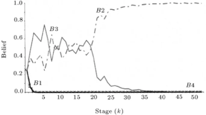
Example 1

Consider S = ff1;f2;f3;f4g, where f1 = Gamma (3;4), f2 = Gamma (12;2), f3 =

Gamma (16;p

3), f4= Gamma (4;2p

3) andBi() = 14

= 0:25. Random numbers have been generated for f2

using Minitab and Steps i to v have been implemented. Results are shown in Figure 1. As seen from Figure 1,

B2 approaches 1 aroundk= 40 illustrating thatf2 is

the winner function.

Figure1. Converging trends of four dierent belief

(3)

Phase Two (Correct Selection)

Step viii

If Bsm;gr(sm;Ok) > :V

sm;gr(k+ 1), then, fx = fgr

is the best t function and one should terminate. Note thatBsm;gr(sm;Ok) can be denoted in a simpler

form of either B(sm;Ok) or Bsm(Ok). Similarly, Bsm;gr(gr;Ok) can be denoted as either B(gr;Ok) or Bgr(Ok). Also, note that :V

sm;gr(k + 1) can be

denoted as :V(k+ 1) for the sake of brevity and is determined by:V(k+ 1) =N kV(N).

Step ix

If Bsm;gr(gr;Ok) < :V

sm;gr(k+ 1), then, fx 6= fgr, so that taking a new observation is required, i.e., if

K N set k = k+ 1, then, go to Step iv; otherwise (i.e., if k > N) stop, then, fx fgr is the best t function and one should terminate.

Step x

IfBsm;gr(sm;Ok)< :V

sm;gr(k+ 1)< Bsm;gr(gr;Ok)

and Bsm;gr(gr;Ok) d

(k), then, f

x = fgr, else,

generate a new observation, i.e., ifKNsetk=k+1, then, go to Step iv; otherwise (i.e., if k > N) stop, then, fx = fgr is the best t function. Note that d(k) is estimated according to a procedure developed in the following section. The complete decision making procedure is also shown in Figure 2.

Phase Three (Estimating

d

(

k

))

Consider d(k) as a decision making criteria or a threshold by which the best t function can be deter-mined eciently. The procedure to determined(k) is considered in the following steps.

Step xi

Deneyxk +1as the most plausible belief onfgr as:

Figure2. Decision making procedure.

yxk +1=Bsm;gr(gr;xk+1;Ok) =

Bsm;gr(gr;Ok):fgr(xk+1)

Bsm;gr(gr;Ok):fgr(xk+1)+Bsm;gr(sm;Ok):fsm(xk+1):

Note that xk+1 has not been generated yet and it is

assumed that it is the best possible observation one can expect to have at the present stage to selectfgr asfx.

Under this assumption, one considers estimating the highest plausible belief one can get on the present best t function, fgr. The underlying idea here is that, if

the next forthcoming observation were considered to be the best possible one, would it be possible to terminate the process and make a decision on a best t function or not? This idea, as illustrated in the following, will help to minimize the need for additional experiments.

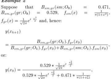
Example 2

Suppose that Bsm;gr(sm;O8) = 0:471, Bsm;gr(gr;O8) = 0:529, fsm(x) = (1+1x2),

fgr(x) = p1 2e x

2

2 and, hence:

y(xk+1)

= _B_sm;gr₍_gr_;_O_kB₎_:fsm;gr_gr₍_x(₉gr₎₊;O_Bk_sm;gr):fgr(₍_smx9)_;_O_k₎_:f_sm₍_x₉₎;

or:

y(x9) = 0:529 1

p 2e

x 2 9 2 0:529

1 p

2e

x 2 9

2 + 0:471

1 (1+x2

9)

;

as illustrated in Figure 3. Note that x9 has not yet

been realized by experimentation, but it is known that its value could only change to the extent shown in Figure 3.

Step xii

Find a derivative of yxk +1, with respect to xk+1, and set this equal to 0, i.e., f0

sm(xk+1):fgr(xk+1) = fsm(xk+1):f0

gr(xk+1), to obtain the roots of the

equa-tion, i.e.,xk+1;t, fort= 0;1;:::l.

(4)

Step xiii

Find yxk +1's for corresponding xk+1;t which are de-noted asy0;y1;;yl (oryt fort= 0;1;l).

Step xiv

Dene the reect lines,yRet, with respect to y = 0:5, asyRet = 1 ytfort= 0;1;

l. Here, at most, 2(l+1) distinct lines can be drawn.

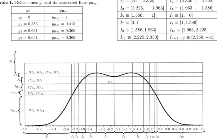
Step xv

Cross yt and yRet lines with a yxk +1 curve and nd the corresponding points onxk+1;t; Hence, the xk+1;t

line is divided into segments which are denoted as

I1;I2;I+1. Also, the yx

k +1 line is divided into segments which are denoted asJ1;J2;Js. Also, Js is denoted as JRes, if Js < 0:5. Note that, for any

Js segment, there could be more than oneIt segment,

where t = 1;2;;+ 1. In the following example, these steps are further illustrated.

Example 3

By setting y0(x

9) = 0, one has x9;1 = 0;x9;2 =

1;x9;3= 1 and the corresponding values foryx9 will be y0 = 0, y1 = 0:585, y2 = 0:631 and y3 = 0:631.

The associated reect lines, with respect to yt's, are

illustrated in Table 1. The values forJss andJRess are also illustrated in Table 2.

Note that, for bothy = 0 andy = 1, there are 7 lines, which, when crossed byy(x9) =B1;3(3;x9;O8),

Table1. Reect linesyt and its associated linesyRe t.

y

t

y

Re

t

y0= 0 yRe

0= 1 y1= 0:585 yRe

1= 0 :415 y2= 0:631 yRe

2= 0 :369 y3= 0:631 yRe

3= 0 :369

Table 2. Values forJss andJRe s.

s

J

s

J

Re

s

1 J1[0:5;0:585] JRe 1

[0:415;0:5]

2 J2[0:585;0:631] JRe 2

[0:369;0:415]

3 J3[0:631;1] JRe 3

[0;0:369] will have the following 11 points (= 11):

xc9;1= 2:350; xc9;2= 2:225; xc9;3= 1:963; xc9;4= 1:586; xc9;5= 1; xc9;6= 0; xc9;7= 1; xc9;8= 1:586; xc9;9= 1:963; xc9;10= 2:225; xc9;11= 2:350:

Sincey(x9) =B1;3(3;x9;O8) is an even function, then,

one has the symmetric roots of xc9;t =xc9;12 t; t=

1;; +1

2 = 6. Now, due to the fact that+ 1 = 12,

one needs to divide thexk+1- axis into 12 segments, as

illustrated in Table 3 and shown, also, in Figure 4. Table3. Values of segments at ions.

I1( 1; 2:350] I2( 2:350; 2:225]

I3( 2:225; 1:963] I4( 1:963; 1:586]

I5[ 1:586; 1] I6[ 1;0]

I7[0;1] I8[1;1:586]

I9[1:586;1:963] I10[1:963;2:225]

I11[2:225;2:350] I+1=12 [2:350;+1]

(5)

Step xvi

For any It segment on the xk+1- axis, dene a

cor-responding JCt segment on the y(xk+1)-axis. This

produces + 1 sub functions, i.e., for any xk+1 2 It andy(xk+1)2JCt.

Step xvii

Collect the monotonically increasing segments in one set,SIn, and the monotonically decreasing segments in

another set,SDe.

Step xviii

Calculate tfort= 1;2;;+ 1, using:

t= Prfxk+12Itg =

Z

It

(Bsm;gr(sm;Ok):fsm(x)

+Bsm;gr(gr;Ok):fgr(x))dx

=Bsm;gr(sm;Ok):

Z

It

fsm(x)dx

+Bsm;gr(gr;Ok):

Z

It

fgr(x)dx:

Note that the function t = 1;2;; +1

2 , if yxk +1 is an even function. This is further illustrated in the following example.

Example 4

Since, for any It segment in the x9- axis, one has a

corresponding JCt segment on the y(x9)-axis, it can

be seen from Figure 4 that:

JC1JRe

3; JC2 JRe

2; JC3 JRe

1;

JC4J1; JC5J2; JC6J2

JC7J2; JC8J2; JC9J1;

JC10JRe

1; JC11 JRe

2; JC12 JRe

3: Now, it is clear that I1, I2, I3, I4, I5 and I7

form the monotonically increasing set,SIn=fIt;8t= 1;2;3;4;5;7gand that I6,I8,I9,I10,I11 andI12 form the monotonically decreasing set, SDe = fIt;8t = 6;8;9;10;11;12g.

Now, one has to calculate the probabilities, t, as

follows:

t=B1;3(1;O8): Z

It

f1(x)dx+B1;3(3;O8): Z

It

f3(x)dx

= 0:471 Z

It 1

(1 +x₂₉)dx+ 0:529 Z

It 1 p

2e

x 2 9 2 dx:

Hence:

1= 12= 0:0652; 2= 11= 0:0049; 3= 10= 0:0269; 4= 9= 0:0168; 5= 8= 0:2476; 6= 7= 0:1386:

Note that y = B1;3(3;x9;O8) is an even function,

so that only six sub functions (i.e., +1₂ ) need to be considered.

Step xix

Draw two lines ofy=dt(k) andy= 1 dt(k) and cross

these two lines withy(xk+1) =Bsm;gr(gr;xk+1;Ok) to

produce the following two corresponding points on the

x-axis,at and bt. Repeat this for t = 1;2;;+ 1. See the following example for better illustrations.

Example 5

To estimate d

s=1(k) for t = 1, for example, two

lines of y = d1(k) and y = 1 d1(k) should be

drawn, as illustrated in Figure 5. Cross these lines withy(xk+1) =Bsm;gr(gr;xk+1;Ok) and produce two

points on the x-axis, denoted asa1 andb1.

Step xx

Construct the following dynamic programming model to maximize the probability of correct selection in the sth segment with k observations (simpler no-tations have been adopted by setting d(J

s;k + 1)

and maxd(Js;n) 2J

s byd

s(k) and maxds(k), respectively. Also,VsmandVgrhave been introduced to simplify the

presentation of the equation. The dynamic model is,

V

s(k) = max_d

t(k)

fVgr+Vsm+:V

(k+ 1) g;

Figure 5. Illustrating an example fory=d 1(

k) and y= 1 d1(k) (Example 5).

(6)

where:

Vgr= [Bsm;gr(gr;Ok) :Vsm;gr(d

t(k+ 1))]

"

X

t Pr(Bsm;gr(gr;xk+1;Ok)dt(k)jxk+12It): t #

; Vsm= [Bsm;gr(sm;Ok) :Vsm;gr(d

t(k+ 1)]

"

X

t Pr(Bsm;gr(gr;xk+1;Ok)1 dt(k)jxk+12It): t #

:

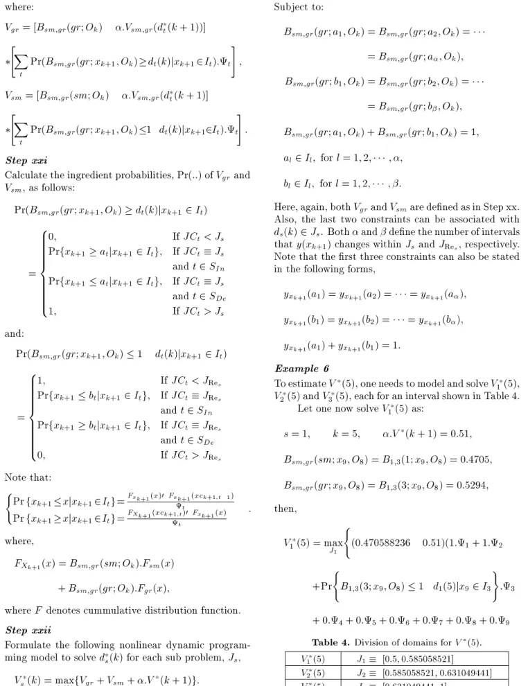
Step xxi

Calculate the ingredient probabilities, Pr(::) ofVgrand Vsm, as follows:

Pr(Bsm;gr(gr;xk+1;Ok)dt(k)jxk+12It)

= 8 > > > > > > > > < > > > > > > > > :

0; IfJCt< Js

Prfxk+1 atjxk+12Itg; IfJCtJs andt2SIn Prfxk+1 atjxk+12Itg; IfJCtJs andt2SDe

1; IfJCt> Js

and:

Pr(Bsm;gr(gr;xk+1;Ok)1 dt(k)jxk+12It)

= 8 > > > > > > > > < > > > > > > > > :

1; IfJCt< JRes

Prfxk+1 btjxk+12Itg; IfJCtJRe s andt2SIn Prfxk+1 btjxk+12Itg; IfJCtJRe

s andt2SDe

0; IfJCt> JRes

Note that: (

Prfxk+1xjxk+12Itg=

Fx

k +1(x) F x

k +1(xc k +1;t 1) t

Prfxk+1xjxk+12Itg=

FX k +1(xc

k +1;t) Fx k +1(x) t

:

where,

FXk +1(x) =Bsm;gr(sm;Ok):Fsm(x) +Bsm;gr(gr;Ok):Fgr(x);

whereF denotes cummulative distribution function.

Step xxii

Formulate the following nonlinear dynamic program-ming model to solved

s(k) for each sub problem,Js, V

s(k) = max_d

t(k)

fVgr+Vsm+:V

(k+ 1) g:

Subject to:

Bsm;gr(gr;a1;Ok) =Bsm;gr(gr;a2;Ok) = =Bsm;gr(gr;a;Ok); Bsm;gr(gr;b1;Ok) =Bsm;gr(gr;b2;Ok) =

=Bsm;gr(gr;b;Ok); Bsm;gr(gr;a1;Ok) +Bsm;gr(gr;b1;Ok) = 1; al2Il; forl= 1;2;;;

bl2Il; forl= 1;2;;:

Here, again, bothVgrandVsmare dened as in Step xx.

Also, the last two constraints can be associated with

ds(k)2Js. Bothanddene the number of intervals thaty(xk+1) changes withinJs andJRes, respectively. Note that the rst three constraints can also be stated in the following forms,

yxk +1(a1) =yxk +1(a2) =

=yx

k +1(a);

yxk +1(b1) =yxk +1(b2) =

=yx k +1(b);

yxk +1(a1) +yxk +1(b1) = 1:

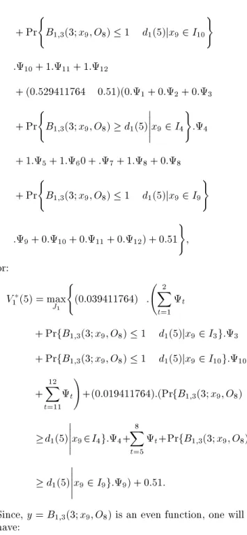
Example 6

To estimateV(5), one needs to model and solveV 1(5), V

2(5) andV

3(5), each for an interval shown in Table 4.

Let one now solveV 1(5) as:

s= 1; k= 5; :V(k+ 1) = 0:51;

Bsm;gr(sm;x9;O8) =B1;3(1;x9;O8) = 0:4705; Bsm;gr(gr;x9;O8) =B1;3(3;x9;O8) = 0:5294;

then,

V

1(5) = max_J 1

(

(0:470588236 0:51)(1: 1+ 1: 2

+Pr (

B1;3(3;x9;O8)1 d1(5)jx92I3 )

: 3

+ 0: 4+ 0: 5+ 0: 6+ 0: 7+ 0: 8+ 0: 9 Table4. Division of domains forV

(5). V

1(5)

J1 [0:5;0:585058521] V

2(5)

J2 [0:585058521;0:631049441] V

3(5)

(7)

+ Pr (

B1;3(3;x9;O8)1 d1(5)jx92I10 )

: 10+ 1: 11+ 1: 12

+ (0:529411764 0:51)(0: 1+ 0: 2+ 0: 3

+ Pr (

B1;3(3;x9;O8)d1(5)

x92I4 )

: 4

+ 1: 5+ 1: 60 +: 7+ 1: 8+ 0: 8

+ Pr (

B1;3(3;x9;O8)1 d1(5)jx92I9 )

: 9+ 0: 10+ 0: 11+ 0: 12) + 0:51 )

;

or:

V

1(5) = max_J 1

(

( 0:039411764): X2

t=1 t

+ PrfB1;3(3;x9;O8)1 d1(5)jx92I3g: 3 + PrfB1;3(3;x9;O8)1 d1(5)jx92I10g: 10 +X12

t=11 t !

+(0:019411764):(PrfB1;3(3;x9;O8)

d1(5)

x92I4g: 4+ 8 X

t=5 t+Pr

fB1;3(3;x9;O8) d1(5)

x92I9g: 9) + 0:51:

Since, y=B1;3(3;x9;O8) is an even function, one will

have: 8 > > > < > > > :

PrfB1;3(3;x9;O8)1 d(1;5)jx92I3g = PrfB1;3(3;x9;O8)1 d1(5)jx92I10g PrfB1;3(3;x9;O8)d1(5)jx92I4g

= PrfB1;3(3;x9;O8)d1(5)jx92I9g

;

so that,V

1(5) can be rewritten as: V

1(5) = max_J 1

(

( 0:078823528):(PrfB1;3(3;x9;O8)

1 d1(5)jx92I3g: 3) + (0:038823528)

:(PrfB1;3(3;x9;O8)d1(5)jx92I4g

: 4) + 0:519468117 )

:

The nonlinear programming model to solve is then,

V

1(5)=maxf( 0:078823528):(FX

9(b) FX9( 2:225)) + (0:038823528):(FX9( 1:586) FX9(a)) + 0:519468117g:

Subject to: (0:8):

f1(a) f3(a)

= (1:125):

f3(b) f1(b)

;

1:963a 1:586; 2:225b 1:963: Now, this problem is solved by writing the program in Lingo [9], as shown in Figure 6.

In writing the Lingo program, shown in Figure 6, the following notes can be helpful:

1. Since the standard normal probability function in Lingo, denoted as @psn(x), can only accept positive values, the negative values have been transformed into positive ones by using ( x) = 1 (x). This is correct, due to the symmetric nature of the normal distribution function;

2. Also, since the Cauchy probability function has not been dened in Lingo, the t-student probability function is used, with one degree of freedom, de-noted as @ptd(n;x) in Lingo, to produce almost the same results. In this case, the t1( x) = 1 t1(x)

transformation is used to produce positive values from negative ones, as thet-student function is also a symmetric function;

(8)

Table5. Finding the optimal decision value.

s J

s

V

s(

k

)

d

s(

k

)

1 J1 V 1(5) = 0

:5197342 d 1(5) = 0

:5402861

2 J2 V 2(5) = 0

:5194529 d 2(5) = 0

:5850582

3 J3 V 3(5) = 0

:51 d

3(5) = 1

:0 The solutions to the non-linear program are:

a= 1:806395; b= 2:091559)V

1(5) = 0:5197342; d

1(5) =B1;3(3;a;O

8) = 1 B1;3(3;b;O 8)

= 0:5404193:

Repeating the above procedure for V

2(5) and V 3(5)

leads to the results illustrated in Table 5 (see [2,3] for details).

Hence,V(k) = max

s=1;2;3fV

s(k)g= 0:5197342, then d(k) =d

1(5) = 0:5402861. This completes the

numerical illustrations.

FURTHER DEVELOPMENTS

In this section, reports are made on further devel-opments of the E-M algorithm. First, parameter optimization of N is considered and, then, a case is considered where both continuous and discrete func-tions can be evaluated in a mixed format.

Parameter Optimization,

N

Parameter optimization is an important element for any ecient algorithm [10] including the E-M algo-rithm. Currently, in the E-M algorithm, the parameter

N, i.e. the number of observations, has not received adequate attention and it is not clear how it could be estimated. IfN is not large enough, then it will not be possible to guarantee the convergence of the algorithm. In other words, smallN may lead to the wrong selection of the candidate function. The question is: How can the value of N be estimated? This is the subject of this Section. Let one start with the following two cases, illustrated in Examples 2 and 3.

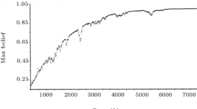
Example 7

Consider the following case, where f4 is the true

candidate function,

f1= Normal (25;100); f2= Normal (21;100); f3= Normal (23;100); f4= Normal (22;100);

f5= Normal (24;100); f6= Normal (20;100):

To simulate this case, 10,000 random numbers have been used, generated by Minitab. The result as illustrated in Figure 7, shows that at least 7000 observations are needed to enable f4 to converge.

Hence, in this case, the parameter, N, should be set around 7000, which is an extremely large number. Intuitively, it can be seen that the large variance, associated with the candidate function, could be a reason.

Example 8

Consider, again, the following case, wheref4is the true

candidate function,

f1= Normal (25;4); f2= Normal (21;4); f3= Normal (23;14); f4= Normal (22;4);

f5= Normal (24;4); f6= Normal (20;4):

The dierence here, with respect to Example 7, is the smaller variance of the corresponding functions. Figure 8 illustrates the converging process. Here, the proper N is about 60 observations, which are drastically smaller than the 7000 observations required in the previous case.

Now that the importance of the right selection of N has been shown, a new procedure is proposed

Figure7. Simulation off4 (Example 7).

(9)

for determining N. Realizing the fact that the set of candidate functions, i.e.,S =f1;f2;fm, are known before, it will be possible to propose the following 3-step procedure for estimatingN:

1. Generate random numbers for ff1;f2;fmg and compute their corresponding belief values fB1();B2();;Bm()g;

2. Compute Nmax _{= max}fNimax; for i = 1;2;mg whenN_imax_{is the maximum number of observations}

needed for convergence offi;

3. SetN=Nmax_.

Now, the working of the above procedure is illustrated in Example 9.

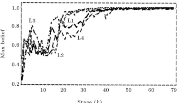
Example 9

Consider the following,

f1= Gamma (3;4); f2= Gamma (12;2); f3= Gamma (16;p

3); f4= Gamma (4;2p 3):

The functions are simulated and their associated belief values are calculated, as shown in Figure 9.

From the curves denoted as L1, L2, L3 and L4 in Figure 9 and, in accordance with Step 2 in the proposed procedure, one hasN₁max50,N2max30,N3max25 and N₄max 50. Hence, according to Step 3 in the proposed procedure,Nmax_{= max}f50;30;25;50g= 50. Therefore, one can safely start the E-M algorithm by settingN = 50.

The above 3-step procedure for estimating N is only taken in a simulated environment and does not eect real experimentation, which may incur cost. It is considered that the proposed procedure should be used as a preprocessing step before application of the E-M algorithm.

It is also noticeable that theNmax_{, as considered}

above, is an upper bound for N_imax_{, ensuring the}

convergence of allfi's. In reality, however, the number

of stages required for the unknown function may be

Figure9. Simulation of converging process (Example 9).

shorter than Nmax_{, so that it is possible to update} Nmax _{adaptively. This means that, by collecting}

any new observation, Nmax should be reestimated.

This may lead, eventually, to N_minmax ₌ _N_i₌_gr _i.e.,

minimizing the total number of observations. In this case, however, the procedure can no longer be applied as a preprocessor but as an integral part of the E-M algorithm. The full development of such an adaptive algorithm is a subject for further research.

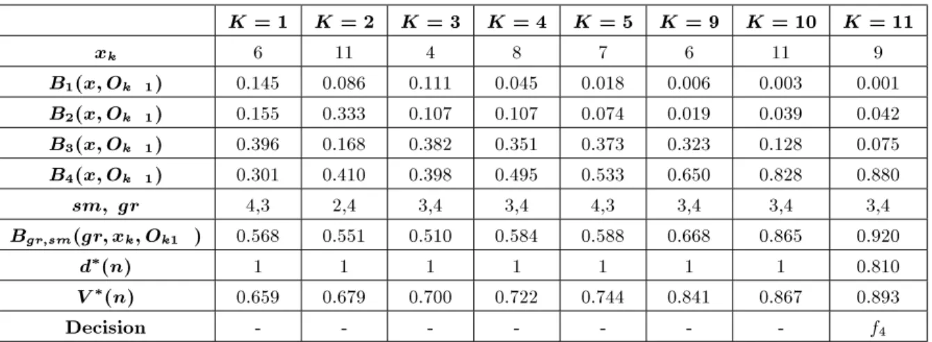
Distribution Fit with Mixed Functions

Theoretically speaking, candidate functions in an E-M algorithm must be of a continuous type. This is naturally a limiting factor in application of the algorithm. In this section, an experiment is per-formed by implementing the method on a problem with both a continuous and a discrete nature, to see if it could work properly. Consider, S = ff1;f2;f4g,

f1 = Exponential (1=8), f2 = Poisson (10), f2 =

Poisson (8), f2 = Poisson (6), N = 12, V(N) = 0:95

and= 0:95 wheref4 is the best t function. Results

are illustrated in Table 6.

As seen from the results illustrated in Table 6, it is clear that the algorithm still selects the best t function correctly. However, theoretical diculties may arise, which demand further investigation. (In a personal discussion with A. Eshragh Jahromi, he warranted the case that belief values, at any stage, may become equal, hence, stalling the process from further advancing. This is avoided in dealing with continuous functions.)

CONCLUSIONS AND FURTHER

RESEARCH

Eshragh and Modarres [1-3] have developed a novel algorithm for a statistical estimation problem, called in this paper, the E-M algorithm. The algorithm uses a new sequential Bayesian method and a stochastic dynamical programming approach to determine when a process of obtaining observations can be stopped. Despite the originality and excellent mathematical analysis developed in the work, the presentation of the algorithm has been very dicult. The E-M algorithm has been presented by a new 3-phase method that illustrates the logical line of the algorithm and its implementation procedures. Finally, the results of our further developments have been resported.

Still, the algorithm can further be developed in some new directions. In order to predict the right candidate function at the present time, the only information being used is the value ofxk. However, it

is quite plausible to introduce further information that can be deriven from a stream ofxk's, including mode,

median, standard deviations and other distribution moments to accelerate the convergence of the algorithm

(10)

4,3 2,4 3,4 3,4 4,3 3,4 3,4 3,4

B

gr;sm(

gr;x

k

;O

k 1

) 0.568 0.551 0.510 0.584 0.588 0.668 0.865 0.920

d

(

n

) 1 1 1 1 1 1 1 0.810

V

(

n

) 0.659 0.679 0.700 0.722 0.744 0.841 0.867 0.893

Decision - - - f

4 by using fuzzy logic and neural networks [11,12]. This

requires further investigations leading to development of a new parallel algorithm for distribution tting problems [13].

ACKNOWLEDGMENT

The authors wish to thank the stimulating discussions with Ali Eshragh Jahromi and Dr. Modarres which helped to develope this paper to the present quality.

REFERENCES

1. Eshragh Jahromi, A. and Modarres Yazdi, M. \Deci-sion on belief: A new approach to distribution tting", First National Conference on Industrial Engineering, Sharif University of Technology, pp 233-283 (in Farsi) (2001).

2. Ranaeifar, F. \Critical Analysis of a new approach to distribution tting: Decision on belief (D.O.B)", Undergraduate Thesis, Industrial Engineering Department, Alzahra University (see the report in http://sta.alzahra.ac.ir/saniee/undergraduatethesis) (2005).

3. Modarres Yazdi, M. and Eshragh Jahromi, A. \De-cision on beliefs: A new approach to distribution tting", Submitted toOperations Research.

4. Shafer, G., A Mathematical Theory of Evidence, Princeton (1976).

5. Dreyfus, S.E. and Law, A.M.,The Art and Theory of Dynamic Programming, Academic Press, Inc. (1977). 6. Ross, S.M., Introduction to Stochastic Dynamic

Pro-gramming, Academic Press, New York, USA (1983). 7. Ahn, J.H. and Kim, J.J. \Action-timing problem with

sequential Bayesian belief revision process",European Journal of Operational Research, 105, pp 118-129

(1998).

8. Conover, W.J., Practical Nonparametric Statistics, 2nd Ed., John Wiley & Sons (1980).

9. Industrial Lingo/P.C., Release 6.0, Lindo Systems, Inc (2000).

10. Monfared, M.A.S. and Yang, J.B. \Sensitivity analysis and parameter optimization",Int. J. of Intelligent and Fuzzy Systems,15(2), pp 89-104 (2004).

11. Monfared, M.A.S. and Steiner, S.T. \Fuzzy adaptive scheduling and control systems",Int. J. Fuzzy Sets and Systems,115, pp 231-246 (2000).

12. Monfared, M.A.S. and Yang, J.B. \Multi level intelli-gent scheduling and control system for an automated ow shop manufacturing environment",Int. J. Produc-tion Research,43(1), pp 147-168 (2005).

13. Monfared, M.A.S. and Khalifeh, F. \Following parallel paths: A new parallel processing algorithm to solve linear programs", Amirkabir Journal of Engineering (in Farsi) (in press).