Sharif University of Technology
Scientia IranicaTransactions E: Industrial Engineering www.scientiairanica.com
A hybrid cultural-harmony algorithm for
multi-objective supply chain coordination
S. Alaei and F. Khoshalhan
Department of Industrial Engineering, KNT University of Technology, Tehran, Iran. Received 2 October 2013; received in revised form 20 April 14; accepted 17 November 2014
KEYWORDS Supply chain coordination; Meta-heuristics; Taguchi method; Supplier selection; Cultural algorithm; Harmony search.
Abstract. We investigate a one-buyer, multi-vendor, coordination model with a vendor selection problem in a centralized supply chain. In the proposed model, the buyer selects one or more vendor and orders an appropriate quantity. The quantity discount mechanism is used by all vendors with the aim of coordinating the supply chain. We formulate the problem as a multi-objective mixed integer nonlinear mathematical model. Using the Global Criterion method, the proposed model is transformed into a single objective optimization problem. Since the problem is NP-hard, we propose four meta-heuristic algorithms: Particle Swarm Optimization (PSO), Scatter Search (SS), population based Harmony Search (HS-pop) and Harmony Search based Cultural Algorithm (HS-CA). The Taguchi robust tuning method is applied in order to estimate the optimum values of parameters. Then, the solution quality and computational time of the algorithms are compared.
c
2015 Sharif University of Technology. All rights reserved.
1. Introduction
Coordination between all entities in a supply chain and global planning is necessary to achieve eective Supply Chain Management (SCM) [1]. In the lack of cooperation, supply chain members are willing to optimize their own objectives independently, which may lead to channel ineciency. Designing mecha-nisms for coordinating and aligning decisions between entities is of great importance in supply chain man-agement. Several coordination mechanisms have been applied in the literature, such as the wholesale price contract [2], two-part tari [3], buyback [4], revenue sharing [5], quantity exibility [6], back-up [7], sales rebate [8], quantity discount [9], timing discount [10], and the revenue sharing reservation contract with penalty [11].
*. Corresponding author. Tel.: +98 21 84063347; E-mail addresses: [email protected] (S. Alaei); [email protected] (F. Khoshalhan)
Supplier (vendor) selection is a strategic decision when a buyer tries to establish a win-win business relationship with its supplier. It is one of the most critical components of the purchasing function of a rm [12]. Vendor selection and order allocation are two main features to be considered in supply chain management.
Suppose a typical channel with a single buyer and multiple vendors. The buyer faces a four-objective constrained problem, i.e. selecting one or more vendor(s) in order to allocate his order quantity for satisfying market demand. All the vendors oer quantity discounts to motivate buyers to order more quantities. The coordination of this supply chain is studied in context to examine the performance of dierent metaheuristic algorithms.
Some models have been developed to investigate the coordination problem and the vendor selection problem. However, little attention has been paid to developing ecient algorithms in this area. In this paper, we consider four metaheuristic algorithms.
The population based Harmony Search (HS-pop) and Harmony Search based Cultural Algorithm (HS-CA) are two hybrid algorithms that are proposed for com-parison with already developed algorithms in this area (i.e. Particle Swarm Optimization (PSO) and Scatter Search (SS)).
The main contributions of the article are: 1. The Harmony Search (HS) algorithm and the
Cul-tural Algorithm are incorporated (CA). We assume that the situational knowledge component of the CA belief space acts as a harmony memory. More-over, ospring are generated using HS operators and CA belief space.
2. In the HS-pop algorithm, the reproduction process and updating the harmony memory are modied compared to the traditional HS algorithm.
The objectives of the research are:
1. To investigate multi-objective coordination of a supply chain using a quantity discount contract; 2. To compare the performance of two hybrid
algo-rithms with other metaheuristic algoalgo-rithms. Using numerical study, we perform analyses over solution qualities and computational eort.
We apply the Taguchi robust tuning method in order to estimate the optimum values of parameters. The Relative Percentage Deviation (RPD) is used to assess the quality of solutions. Moreover, in order to evaluate the computational time of the proposed algorithms, the time to reach a solution with r% error (i.e. 1% or 3%) is computed. We investigate the Convergence Index (CI) of the proposed algorithms, as the number of successful runs with which the algorithm reaches a solution, with r% error, over the total number of runs.
The remainder of the paper is organized as fol-lows: Section 2 briey reviews the related literature. Section 3 describes the problem and notation. Section 4 presents the solution procedure and four metaheuristic algorithms. In Section 5, the Taguchi method is used for tuning parameters of the algorithms. Section 6 provides an illustrative example. The proposed algo-rithms are evaluated using the numerical example in Section 7. Finally, Section 8 summarizes and concludes the paper.
2. Literature review
We provide a brief review of supply chain coordi-nation and supplier selection models that have been studied in recent years. Rosenthal et al. [13] studied a supplier selection problem with multiple products, where suppliers oer discounts when a \bundle" of products is bought. Sarkis and Semple [14] discussed a single period supplier selection problem with business
volume discounts, wherein the total purchasing cost should be optimized without taking inventory-related costs into account. Goossens et al. [15] studied a multi items supplier selection, wherein the suppliers oer an all-unit quantity discount and try to mini-mize the total cost of purchasing. Ghodsypour and O'Brien [16] developed an integrated AHP and linear programming model, in which both qualitative and quantitative factors are considered in the process of supplier selection and order allocation. Amid et al. [17] proposed a weighted additive fuzzy multi-objective model for the supplier selection problem under all-unit price discounts.
Jayaraman et al. [18] developed a Mixed Integer linear Programming (MIP) model, wherein quality production capacity, lead-time, and storage capacity limits are considered. Another MIP model for the supplier selection is proposed by Cakravastia et al. [19] where the objective is to minimize the level of customer dissatisfaction, which was evaluated by price and lead time. Dahel [20] developed a Multi-Objective Mixed Integer Programming (MO-MIP) model with multiple products and discounts on total business volume. Xia and Wu [21] presented a MO-MIP approach under a total business volume discount, and used an integrated AHP method and multi-objective programming to investigate the problem. Ebrahim et al. [22] developed a MO-MIP model with dierent types of discount and proposed a scatter search algorithm to solve the problem.
Herer et al. [23] were the rst to propose a supplier selection problem together with coordination models. The limited annual production rate and inventory holding costs are taken into account in their model. Kim and Goyal [24] investigated two dierent shipment policies from the suppliers to the buyer in which suppliers deliver their production lots either simultaneously or successively. Kamali et al. [25] developed a multi-objective mixed integer nonlinear programming model to coordinate the system of a single-buyer- multi-vendors, under an all-unit quantity discount. They proposed Particle Swarm Optimization and Scatter Search for solving the problem. Gheidar-Kjeljani [26] proposed a nonlinear mathematical model which is a combination of a supplier selection model and a coordination model in a centralized supply chain. In their model, the buyer ordered quantities are split into small lot sizes and are delivered to the buyer over multiple periods.
3. Problem description
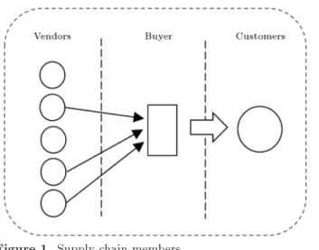
A typical channel with one buyer and multiple vendors is considered. The buyer selects one or more vendors in order to allocate his order quantity for satisfying market demand without any type of shortage. All the
Figure 1. Supply chain members.
vendors oer quantity discounts to motivate buyers to order more quantities. A schematic view of the supply chain is illustrated in Figure 1. Selecting suitable vendors for supplying the products is an important part of the operation.
The buyer has to choose one or more vendor(s) and purchase an optimal level of single product from each vendor based on various objectives. The buyer has a dilemma, due to discount contracts oered by the vendors, which depend on the volume of the order quantity. The objectives considered in this paper for choosing potential vendors are similar to those of Kamali et al. [25]; they are:
a) Minimizing the whole supply chain annual costs; b) Minimizing the total defective items ordered by the
buyer;
c) Minimizing the total late delivered items; d) Maximizing the total annual purchasing value. Suppose that there are n vendors in the supply chain. Each of them (i.e., vendor i) oers an all-unit quantity discount with Ki price level, each level (i.e. level k) is
characterized by an interval, [ui;k 1; uik), and the price
of cik is associated with this interval. For example, for
each vendor, i, we have ui1 < ui2 < < ui;Ki and
ci1> ci2> > ci;Ki. Also, assume that vendor order
quantities are dispatched to the buyer in a sequential order. In other words, after consuming the products of one vendor, the products of another vendor can be entered.
Parameters used in the problem:
D Buyer annual xed market demand rate;
Si Fixed setup cost associated with
vendor i;
Ai Buyer xed ordering cost for vendor i;
hi Vendor i's inventory holding cost per
unit, per unit time;
h Retailer's xed inventory holding cost per unit, per unit time (independent of purchasing cost);
Ti Consumption time of an order quantity
from vendor i;
T Cycle time of the retailer; zi Unit variable cost of vendor i;
Pi Production rate associated with vendor
i;
bik Quantity at which the kth price break
occurs by vendor i;
Ri Reliability of time of delivery of
products for vendor i;
di Defective rate that vendor i maintains;
wi Total weight assigned to vendor i.
Decision variables used in the model:
qik Number of units supplied by vendor i
at price level k in a cycle;
yik Binary variable denoting whether order
quantity is chosen from k's price level or not;
Qi Order quantity supplied by vendor i in
a cycle, i.e. Qi=PKk=1i qik;
Q Total order quantity supplied by all vendors in a cycle, i.e. Q =Pni=1Qi.
The problem consists of four objectives:
a) Cost: To minimize annual costs of the whole supply chain:
Z1=DQ n
X
i=1 Ki
X
k=1
(zi+ cik)qik
+DQ
n
X
i=1 Ki
X
k=1
(Ai+ Si)yik
+DQ
n
X
i=1
2 41
2
h D +
hi
Pi
XKi
k=1
qik
!23
5 : (1) The objective function, as shown in Eq. (1), con-sists of three parts: The rst part includes variable and purchasing costs; The second part consists of ordering and setup costs; and the third part includes buyer and vendor holding costs.
b) Quality: To minimize the total defective items ordered by the buyer:
Z2= DQ n
X
i=1 Ki
X
k=1
c) Delivery reliability: To minimize the total late delivered items:
Z3= DQ n
X
i=1 Ki
X
k=1
(1 Ri)qik; (3)
where (1 Ri) denotes the late delivery rate of
products for vendor i.
d) Purchasing value: To maximize the total annual purchasing value:
Z4= DQ n
X
i=1
wi Ki
X
k=1
qik; (4)
where wi captures the overall performance of
ven-dor i, and can be calculated by multiple criteria decision making methods; andPKi
k=1qikis the total
amount of products to be ordered from vendor i. Note that the vendor with the highest weight has a higher priority for purchasing. In a single objective framework, the decision maker (buyer) tends to purchase all his order quantities from the vendor with the highest weight. So, maximizing Eq. (4) ensures that the greater part of the buyer orders are allocated to vendors with higher performance weights and higher priorities.
Under the Global Criterion method, the relative weighted distance between each objective function's value and its reference point is minimized. The reference point for each objective m (Z
m), is obtained
by optimizing the mth objective and neglecting other objectives subject to the problem constraints. Suppose that Wm is the weight of objective m that can be
achieved by decision maker preferences. So, the prob-lem can be rewritten as the following single objective optimization problem:
min Z =
4
X
m=1
WmjZm Z mj
Z
m : (5)
Moreover, the problem has the following constraints: Capacity constraint: Each vendor, i, has maximum
capacity, D Q
Ki
X
k=1
qik Pi 8i = 1 n: (6)
Demand constraint: The demand of the buyer has to be satised,
n
X
i=1 Ki
X
k=1
qik= Q: (7)
Discount constraints: The following constraints ensure that if vendor i is chosen, the amount of order quantity should fall into discount interval [ui;k 1; uik):
Ki
X
k=1
yik 1 8i = 1 n; (8)
ui;k 1yik qik uikyik
8i = 1 n; 8k = 1 Ki: (9)
4. Solution procedure
For the problem studied in this paper, we investigate four algorithms. As mentioned before, they are PSO, SS, HS-pop and HS-CA. Here, each solution vector is demonstrated as Q = [Q1; Q2; ; Qn], where Qi is
the order quantity assigned for vendor i, and is equal to Qi = [qi1; qi2; ; qiKi]. In all algorithms studied
here, we apply a similar algorithm for generating initial solutions. In this algorithm, each vendor is selected with a probability of 0.5. Then, for each selected vendor, i, an order quantity is randomly assigned between [0; uik).
4.1. Repair algorithm
In order to avoid infeasible solutions caused by capacity constraints, we apply repairing strategies in all algo-rithms. A repair procedure transforms an infeasible solution into a feasible one. For the problem studied in this paper, if each vendor annual capacity constraints are violated by assigned annual order quantities, then, the extra amount of their order quantities is assigned to other vendors by a rule, as described below.
For any infeasible solution, we dene ai = Pi
DQi=Q for each vendor, i, in which ai 0 points
out that vendor i still has some capacity for assigning the order, and ai < 0 indicates that the annual
order quantity allocated to vendor i exceeds its annual production capacity. Then, we dene two subset of vendors as S+ = fi : a
i 0g, which captures vendors
that still have some capacity, and S = fi : ai < 0g,
which demonstrates vendors with violated capacity constraints. So, the following changes ensure the feasibility of the solution until we have Pi2S+ai
P
i2S ai, otherwise, the solution should be rejected:
Qi=DQPi 8i 2 S ; (10)
Qi= Qi+
ai
P
i2S+ai
X
i2S
ai 8i 2 S+: (11)
Eq. (10) sets the annual order quantity of already-capacity-violated vendors to be equal to their annual
production capacity. Eq. (11) shares the extra quantity (Pi2S ai) among the other vendors proportional to
their remainder capacity.
4.2. Particle swarm optimization
Particle swarm optimization is a population based metaheuristic inspired from swarm intelligence [27]. PSO has been successfully applied for continuous op-timization problems [28]. A swarm of N particles ies around the search space. Each particle position is determined by its velocity and previous position. The step and direction of each particle, i, toward the global optimum is aected by two factors: P besti, which is
the best position visited by itself; and Gbest, which is the best position visited by all particles. The velocity of each particle is updated as follows:
vt+1
i =w vit+ c1 r1 (P bestti xti) + c2
r2 (Gbestt xti); (12)
where r1; r2 2 [0; 1] are two random numbers; c1 and
c2are constant and denote the learning factors; t is the
iteration number; and w is the inertia weight which controls the eect of previous velocity on the current one. We use a dynamic approach for the inertia weight, as:
w(t) = wmax wmaxNwmin t; (13)
where wminand wmaxare the minimum and maximum
inertia weights, respectively, and N is the maximum number of iterations. Then, each particle position is updated with:
xt+1
i = xti+ vit+1: (14)
At each iteration, the values of P besti and Gbest are
updated if better solutions are obtained by particle i and all particles, respectively. Algorithm 1 presents the template for PSO.
4.3. Scatter search
The scatter search was rstly introduced by Glover [29] and is an evolutionary metaheuristic which recombines selected solutions from a reference set to build oth-ers [30]. There are ve basic methods in the scatter search [31]:
Algorithm 1. Particle Swarm Optimization (PSO) pseudo code.
1. A Diversication generation method generates a set of diverse trial solutions. This method aims to diversify the search while selecting high-quality solutions.
2. An Improvement method transforms a trial solution into one or more enhanced trial solutions using any S-metaheuristic. Usually, a local search algorithm is applied and then a local optimum is generated. 3. In the Reference set update method, the aim is
to guarantee diversity while keeping high-quality solutions. This method builds and maintains a reference set (with b individuals) that consists of two subsets: Ref-Set1 (with b1 individuals), with
the best tness function, and Ref-Set2 (with b2
individuals where b2 = b b1), with the best
diversity.
4. A Subset Generation Method operates on the ref-erence set, and produces a subset of solutions as a basis for creating combined solutions. In this method, all the subsets of a xed size, r (generally, r = 2), are selected.
5. The Solution Combination Method is a given subset of solutions produced by the Subset Generation Method transformed into one or more combined solution vectors.
Algorithm 2 presents the template for SS. 4.4. Proposed algorithms
4.4.1. Brief review of harmony search
Harmony Search (HS), a relatively new metaheuristic optimization algorithm, was introduced by Geem et al. [32]. It imitates musician behavior, where the instrument pitch is improvised upon by searching for a perfect state of harmony. According to the harmony search algorithm, the Harmony Memory (HM) is a matrix of individuals with a size of HMS:
HM = 2 6 4
Q1
... QHMS
3 7 5 =
2 6 4
q11 qn1
... ... ... q1;HMS qn;HMS
3 7
5 ; (15)
where we have f(Q1) f(Q2) f(QHMS). In
order to update HM, if a new generated solution is better than the worst vector, then, the worst vector is replaced by the new one.
A new harmony vector or individual is generated by considering harmony memory and randomness. q0
i
( q0
i2fqi1; qi2; ; qi;HMSg w.p. HMCR
q0
i2Ai w.p. (1 HMCR) (16)
Pitch adjusting for: q0
i
(
Yes w.p. PAR No w.p. (1 PAR) q0
i qi0 rand() bw; (17)
where HMCR 2 [0; 1] is the Harmony Memory Con-sidering Rate; PAR 2 [0; 1] is the Pitch Adjustment Rate; and bw is the maximum distance bandwidth of changing q0
i. At each iteration:
1. Each new variable either inherits its value from the historical values stored in HM with a probability of HMCR, or is chosen according to its possible range, with a probability of (1-HMCR).
2. Then, each decision variable is examined as to whether or not to be changed around its value, with a probability of PAR.
In this paper, we use the improved version of Harmony Search (IHS) proposed by Mahdavi et al. [33]. Their proposed algorithm includes dynamic adaptation for both PAR and bw values. The PAR value is linearly increased, and the bw value is exponentially decreased in each iteration of the HS using the following equa-tions, respectively:
PAR(t) = PARmin+PARmaxNIPARmin t; (18)
bw(t) = bwmax exp(c t);
c = Ln(bwminNI=bwmax); (19) where PARmin and PARmax are the minimum and
maximum pitch adjusting rates, respectively, NI is the maximum number of iterations, t is the generation number; bwmin and bwmax are the minimum and
maximum bandwidths, respectively. 4.4.2. Brief review of cultural algorithm
Cultural Algorithms (CAs) were introduced by Reynolds [34] and are special variants of evolutionary algorithms. They are inspired by the principle of cultural evolution. The CA framework consists of
population space and belief space, which is used for forming, storing, and delivering knowledge experiences. The belief space contains the ve knowledge sources, i.e. the normative, situational, domain, to-pographical and history KS. Here, we apply two kinds of the most fundamental knowledge of the belief space: situational knowledge, St, and normative knowledge,
Nt. That is, Bt = (St; Nt), where the situational
knowledge, St, is the set of best individuals. For
exam-ple, for K best individuals, the situational knowledge has the following structure:
St=
2 6 6 6 6 6 4
x1
1; x12; ; x1n; f(x)1
x2
1; x22; ; x2n; f(x)2
... xK
1 ; xK2 ; ; xKn; f(x)K
3 7 7 7 7 7
5: (20)
Moreover, the normative knowledge, Nt, is the set of
interval information, together with the tness for each extreme of the interval:
Nt= Xt
1; X2t; ; Xnt
; (21)
and for each domain variable, Xt
i, the following
infor-mation is stored: Xt
i = (lti; uti; Lti; Uit); i = 1 n; (22)
where lt
i and uti, respectively, represent the lower and
upper bounds of the closed interval for variable i, i.e. lt
i qi uti; Lti and Uit are the performance scores
of the individual for the lower and upper bounds, respectively.
There are two main phases in the CA: the inu-ence phase and the acceptance phase. The inuinu-ence function determines which knowledge source inuences individuals. The original CA used the roulette wheel selection, based on knowledge source performance in previous generations [35]. The acceptance function de-cides which individuals and their properties can aect the belief space [36]. For example, a percentage of the best individuals (e.g. top 10%) can be accepted [36].
With the acceptance function and inuence func-tion on hand, the belief space is updated at each generation. Updating the situational knowledge can be done by any selection approach. For example, one can update situational knowledge by the k top individuals in the population, or use the Tournament selection.
In addition, the normative knowledge of belief space is updated at each generation. The lower and upper boundaries of decision variables and their responding tness values are updated as follows. For each Qt
j; j = 1::nBt;
lt+1 i =
( qt
ij if qijt litor f(Qtj) < Lti
lt
Figure 2. Procedure of the proposed HS-pop algorithm.
ut+1i = (
qt
ij if qijt uti or f(Qtj) < Uit
ut
i otherwise (24)
Lt+1 i =
( f(Qt
j) if qijt litor f(Qtj) < Lti
Lt
i otherwise
(25)
Ut+1 i =
( f(Qt
j) if qijt uti or f(Qtj) < Uit
Ut
i otherwise (26)
4.4.3. Population based harmony search (HS-pop) In a traditional harmony search, only one new harmony vector or individual is generated during the reproduc-tion process, and only one individual is examined in order to update the harmony memory. However, in this algorithm, a population based approach is applied in the harmony search algorithm. In other words, K new harmonies are generated at each generation. At each generation, as illustrated in Figure 2, K new individuals are generated with the following rules: a) K0 best individuals are selected from the previous
population, K0 < K. We assume that these
indi-viduals form the harmony memory (K0 = HMS);
b) Then, (K K0) ospring are generated based on
harmony search operators, i.e. PAR and HMCR. Algorithm 3 presents the template for HS-pop. 4.4.4. Harmony search based cultural algorithm
(HS-CA)
Gao et al. [37] proposed a hybrid optimization method in which the HS algorithm is merged together with CA. First, the knowledge of the belief space is extracted from the harmony memory, and then used to direct the mutation of the new ospring. Using the historical values of individuals, we incorporate the HS algorithm into CA. We assume that the situational knowledge
Algorithm 3. Population based harmony search (HS-pop) pseudo code.
Algorithm 4. Harmony search based cultural algorithm (HS-CA) pseudo code.
Figure 3. Procedure of the proposed HS-CA algorithm.
component of the CA belief space acts as a harmony memory matrix with the size of HMS. The procedure of the algorithm is illustrated in Figure 3. Here, all steps of the algorithm are similar to those of Algorithm 3, except for the reproduction process. Algorithm 4 presents the template for HS-CA.
The procedure of Algorithm 4 is described below in detail.
Initialization: The rst population, including K solution vectors, is generated. Suppose that we denote the mth solution vector at iteration t with Qt
m =
[Qt
the order quantity assigned for vendor i at iteration t, and n is the number of vendors. For each solution vector, an order quantity for vendor i is randomly chosen from its production interval. That is, Q0
mi= an
integer random number, 2 [0; ui], i = 1; 2; ; n, m =
1; 2; ; K. Then, infeasible solutions are transformed to feasible ones by repairing the algorithm described in Section 4.1. All the individuals are evaluated by the tness function, f(:), and sorted, in ascending order, according to their tness value in P op0:
P op0=
2 6 6 6 4 Q0 1 Q0 2 ... Q0 K 3 7 7 7 5= 2 6 6 6 4 Q0
11 Q012 Q01n
Q0
21 Q022 Q02n
... ... ... ... Q0
K1 Q0K2 Q0Kn
3 7 7 7
5; (27) where Q0
1 and Q0K are the best and worst solutions,
respectively, and we have f(Q0
1) f(Q02)
f(Q0
K). Recall that the belief space comprises
norma-tive knowledge and situational knowledge. Normanorma-tive knowledge is denoted by Nt= (Xt
1; X2t; ; Xnt), where
Xt
i = (lti; uti; Lti; Uit). Note that the closed interval
characteristic for each vendor is initialized as below: l0
i = 0; u0i = ui; L0i = 1; Ui0= 1;
i = 1 n: (28)
We assume that at each generation, K0 best
individ-uals from the previous generation form the harmony memory matrix, with HMS being equal to K0 (where
K0 < K). So, situational knowledge is initialized as
below: S0=
2 6 6 6 4 Q0
11 Q012 Q01n
Q0
21 Q022 Q02n
... ... ... ... Q0
K0;1 Q0K0;2 Q0K0;n
3 7 7 7
5: (29)
Reproduction: The hybrid HS-CA applies elitism for K0the best individuals, in order to keep them from
one generation to the next. The remaining (K K0)
individuals are generated based on harmony search operators, i.e. PAR and HMCR, as described in the following.
With an inuence function, the knowledge in the belief space can be used to inuence the creation of the ospring. We assume that both normative and situational (harmony memory) components are used during the ospring generation. Each variable in the new harmony vector or individual is generated as below: Qt :i 8 > > > > > > < > > > > > > : Qt
:i2 fQt 11i ; Qt 12i ; ; Qt 1K0ig
w.p. HMCR Qt
:i= Qt 1:i + (ut 1i lt 1i )Ni(0; 1)
w.p. (1 HMCR)
(30)
where HMCR 2 [0; 1] is the Harmony Memory Consid-ering Rate. Note that each variable of an individual is generated using either situational knowledge with the probability of HMCR, or normative knowledge with the probability of (1-HMCR). Then, each decision variable is examined as to whether or not be changed around its value, with a probability of PAR, using the following formula:
Pitch adjusting for: Qt
:i
(
Yes w.p. PAR No w.p. (1 PAR) Qt
:i Qt:i rand() bw; (31)
where PAR 2 [0; 1] is the Pitch Adjustment Rate, and bw is maximum distance bandwidth of changing qt
i.
Updating the belief space: We use the dynamic formula (32) to determine how many individuals should be selected from the P opt in order to shape the belief
space: nBt =
K
t
; 2 [0; 1]; (32)
where t is the iteration number. These nBt best
performers are selected to update the normative knowl-edge, i.e. for each Qt
mi; m = 1 nBt; i = 1 n,
Eqs. (23)-(26) should be updated. Moreover, the situational knowledge or harmony memory (St =
HMt) should be updated by replacing the previous
individuals by K0 best individuals.
5. Parameters tuning
The parameters of the algorithms impress the solution quality. There are several ways of tuning the parame-ters. One is the Taguchi method. The Taguchi robust tuning method is a powerful tool in the DOE (design of experiment), in order to estimate the optimum values of parameters. This method applies the S/N (signal to noise) ratio for measuring the quality characteristics deviating from the desired values.
There are three categories in S/N ratio per-formance evaluations, depending on the goal of the problem, i.e. smaller-the-better, larger-the-better, and nominal-the-best. In this paper, the smaller-the-better quality characteristic is taken into account with the following formula:
S=N = 10 log 1n
n X i=1 y2 i ! ; (33)
where y is the observed tness, and n is the number of observations. Here, we use the Taguchi method only for tuning parameters of HS-pop and HS-CA. For SS and PSO parameters, please refer to Kamali et al. [25].
Table 1. Optimal levels of PSO's parameters. Swarm-size Wmin Wmax c1 c2 Optimal level 100 0.2 0.7 0.8 0.8
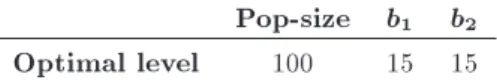
Table 2. Optimal levels of SS's parameters. Pop-size b1 b2 Optimal level 100 15 15
5.1. PSO and SS parameters
Kamaliet al. [25] applied the Taguchi method for parameter tuning, and determined appropriate levels for each algorithm parameter. The best levels of parameter for PSO and SS are summarized in Tables 1 and 2.
5.2. Tuning HS-pop parameters
Here, by applying the Taguchi method, we evaluate the impact of seven parameters on the output parameter (tness function). These parameters and their levels are shown in Table 3. There are seven parameters, and each one has three levels. In order to conduct the experiment, the appropriate orthogonal array is L18(37 21), which is tabulated in Table 4. Since
the selected array has one additional parameter with 2 levels (P1), the additional parameter column can be easily ignored from the experiment.
Taking the full factorial model into account, 37 = 2187 dierent combinations for each problem
are reduced to 18 problems using the Taguchi method. In order to reduce experimental error, we repeat each experiment 5 times. The ANOVA test on the S/N ratio with 99.5% condence limit is implemented and the re-sults are shown in Table 5. The ANOVA indicates that Pop-size, HMS, HMCR and PARmax (with P -values
lower than 0.005) are the most signicant parameters. These four parameters have the most sensitivity eect on the quality of solution, and other parameter impacts can be ignored.
The results of ANOVA indicate that there are no major dierences between the levels of that parameter for each insignicant parameter. However, the level with the highest S/N ratio is the optimal level. Ta-ble 6 indicates the average S/N ratio for parameters. The signicance of the parameters is calculated by the dierence between max and min values for each parameter. As shown in Table 6, Pop-size gets the rst
Table 4. Experimental plan using L18orthogonal array. Parameters
P1 P2 P3 P4 P5 P6 P7 P8
Exp
erimen
ts
1 1 1 1 1 1 1 1 1
2 1 1 2 2 2 2 2 2
3 1 1 3 3 3 3 3 3
4 1 2 1 1 2 2 3 3
5 1 2 2 2 3 3 1 1
6 1 2 3 3 1 1 2 2
7 1 3 1 2 1 3 2 3
8 1 3 2 3 2 1 3 1
9 1 3 3 1 3 2 1 2
10 2 1 1 3 3 2 2 1
11 2 1 2 1 1 3 3 2
12 2 1 3 2 2 1 1 3
13 2 2 1 2 3 1 3 2
14 2 2 2 3 1 2 1 3
15 2 2 3 1 2 3 2 1
16 2 3 1 3 2 3 1 2
17 2 3 2 1 3 1 2 3
18 2 3 3 2 1 2 3 1
Table 5. ANOVA results for S/N ratio of Pop-HS. Source DF ANOVA
SS
Mean
squares F -value P -value Pop-size 2 0.0451 0.0226 704.5 0:0001 HMS 2 0.0107 0.0053 166.3 0:0008
HMCR 2 0.0048 0.0024 75.4 0:003
PARmin 2 0.0019 0.0010 29.8 0.010 PARmax 2 0.0052 0.0026 81.6 0:002 bwmin 2 0.0008 0.0004 11.8 0.038 bwmax 2 0.0011 0.0006 17.8 0.022 Error 3 0.0001 0.00003
Total 17 0.0698
highest value, HMS gets the second highest value, and so on. Hence, this result conrms the ANOVA results. In order to determine the optimal levels of sig-nicant parameters, including Pop-size, HMS, HMCR and PARmax, the SNK (Student-Newman-Keuls) range
test is applied and the results show that there is no signicant dierence between levels 2 (75) and 3 (90) of
Table 3. Introducing levels of parameters for Pop-HS.
Pop-size HMS HMCR PARmin PARmax bwmin bwmax
Level 1 50 15 0.9 0.1 0.6 1 10
Level 2 75 30 0.93 0.15 0.75 5 20
Table 6. Average S/N ratio and signicance of Pop-HS parameters.
Pop-size HMS HMCR PARmin PARmax bwmin bwmax
Level 1 18.022 18:122 18.073 18.080 18.083 18:101 18:103 Level 2 18:128 18.094 18.092 18.094 18:117 18.092 18.090 Level 3 18.128 18.062 18:113 18:105 18.078 18.085 18.084 Signicance 0.107 0.060 0.040 0.025 0.038 0.017 0.019 Figure
Table 7. Optimal levels of Pop-HS parameters.
Pop-size HMS HMCR PARmin PARmax bwmin bwmax
Optimal level 75 15 0.96 0.25 0.75 1 10
Table 8. Introducing levels of parameters for HS-CA.
Pop-size HMS HMCR PARmin PARmax bwmin bwmax
Level 1 50 15 0.9 0.1 0.6 10 500
Level 2 75 30 0.93 0.15 0.75 100 1000
Level 3 90 40 0.96 0.25 0.9 500 2000
Pop-size, but the S/N ratio of level 1(50) is signicantly smaller than that of levels 2 and 3. So, we choose level 2 (75) for reducing computational time. Furthermore, there are no signicant dierences between levels of HMS, HMCR and PARmax. So, for each parameter,
we choose the level that gets the higher S/N ratio. We repeat the experiments for n = 4 and derive the ANOVA results again. Results indicate similar levels for parameters. We conclude that the optimal levels for the parameters are as in Table 7.
5.3. Tuning HS-CA parameters
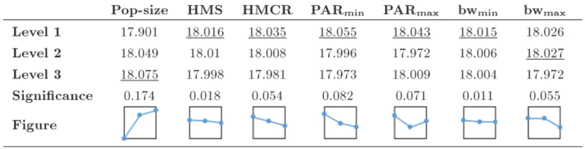
Here, similar to the previous subsection, there are seven parameters, and each one has three levels. These parameters and their levels are shown in Table 8. Table 9 summarizes the ANOVA test on S/N ratio with 99.5% condence limit. It is obvious that Pop-size is the most signicant parameter. We use the SNK test
Table 9. ANOVA results for S/N ratio for HS-CA. Source DF ANOVA
SS
Mean
squares F -value P -value Pop-size 2 0.1053 0.0526 49.78 0.005
HMS 2 0.0009 0.0005 0.44 0.678
HMCR 2 0.0087 0.0043 4.10 0.139 PARmin 2 0.0213 0.0106 10.05 0.047 PARmax 2 0.0150 0.0075 7.11 0.073 bwmin 2 0.0004 0.0002 0.19 0.833 bwmax 2 0.0121 0.0060 5.72 0.095 Error 3 0.0032 0.0011
Total 17 0.1668
for Pop-size, and other parameter optimal levels are determined based on the value of S/N ratio, which are tabulated in Table 10. So, the optimum level of each parameter is shown in Table 11.
6. Illustrative example
Suppose that a single buyer would like to purchase a product from 4 vendors. The same data as in Kamali et al. [25] is used here. The annual market demand is 100,000, and the unit holding cost per time unit (hb)
is 2.6. Table 12 summarizes vendor information. Also, Table 13 gives the information about the vendor oered quantity discount. Moreover, the optimal values of each objective, by neglecting the other objectives, are Z = (1488623; 1813:621; 13822:47; 60744:51). Also,
the decision maker preferences about weights on the objectives are: W = (0.4, 0.1, 0.2, 0.3).
Table 14 shows that all algorithms result in almost the same value for each objective function. However, our proposed HS-CA algorithm yields a slightly better overall objective function (Z), by 0.04% over that of Kamali et al. [25]. Moreover, the order quantities obtained by our PSO and Pop-HS coincide with the results of Kamali et al. [25], but, SS and HS-CA result in dierent order quantities with better overall objective function.
7. Performance comparison of algorithms For evaluating the performance of the proposed al-gorithms, we generate four problems with a dierent number of vendors, i.e. n = 5, 10, 15 and 20. Then,
Table 10. Average S/N ratio and signicance of HS-CA parameters.
Pop-size HMS HMCR PARmin PARmax bwmin bwmax Level 1 17.901 18:016 18:035 18:055 18:043 18:015 18.026 Level 2 18.049 18.01 18.008 17.996 17.972 18.006 18:027 Level 3 18:075 17.998 17.981 17.973 18.009 18.004 17.972 Signicance 0.174 0.018 0.054 0.082 0.071 0.011 0.055 Figure
Table 11. Optimal levels of HS-CA parameters.
Pop-size HMS HMCR PARmin PARmax bwmin bwmax
Optimal level 75 15 0.9 0.1 0.6 10 1000
Table 12. Vendors' information. Vendor
1 2 3 4
z 4.04 6.48 7.17 5.87
S 43 39 42 30
P 35108 29898 35785 68777
A 40 19 25 39
h 2.29 1.96 2.74 0.54
d 0.0344 0.0551 0.0121 0.0215 H 0.1444 0.1806 0.116 0.1581 w 0.7968 0.3629 0.326 0.505
we run each algorithm ten times for each problem. In order to assess the quality of solutions, we use the Relative Percentage Deviation (RPD) as a performance measure, that is:
RPD = fff 100; (34)
where fis the global optimum or best known solution,
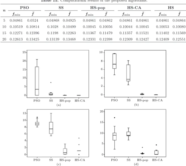
and f is an obtained solution for an instance. Table 15 shows the objective function values. It can be inferred from Table 15 that the HS-pop and HS-CA perform better than standard HS, and they all perform better than SS and PSO in nding best solutions. In order to better compare each algorithm performance, the RPD of each algorithm for each problem size is computed and illustrated by a box plot, as in Figure 4.
It can be implied from Figure 4 that HS-pop and HS-CA perform better than Scatter Search and Particle Swarm optimization algorithms; both in best known solutions and solution variability.
In order to evaluate the computational time of the proposed algorithms, the time to reach a solution with r% error is computed, where r is the maximum value of average RPD of dierent algorithms for given n. The value of r for n = 5, 10, 15 and 20 is equal to 7.8, 7.7, 9.2 and 9.4, respectively. We dene the Convergence
Table 13. Discount intervals oered by vendors. Vendor Intervals Unit prices
1
(0, 5000) 9
[5000, 10000) 8.9 [10000, 15000) 8.8 [15000, 20000) 8.7 [20000, 25000) 8.6 [25000, 30000) 8.5 [30000, 35108) 8.4
2
[0, 2000) 9.1
[2000, 4000) 9 [4000, 6000) 8.9 [6000, 8000) 8.8 [8000, 10000) 8.7 [10000, 20000) 8.6
3
[0, 3000) 8.7
[3000, 6000) 8.6 [6000, 9000) 8.5 [9000, 12000) 8.4 [12000, 15000) 8.3 [15000, 18000) 8.2 [18000, 21000) 8.1 [21000, 30000) 8
4
[0, 4000) 10.5
[4000, 8000) 10.4 [8000, 12000) 10.3 [12000, 16000) 10.2 [16000, 68777) 10.1
Index (CI) as the number of successful runs in which the algorithm reaches a solution with r% error in a time less than 300 seconds, over the total number of runs.
CI = number of successful runs
total number of runs : (35)
Table 14. Optimal solution for base data.
HS Pop-HS HS-CA SS PSO Kamali et al. [25]
Z 0.063098 0.063098 0.063064 0.063087 0.063095 0.063095 Z1(106) 1.5128 1.5128 1.5127 1.5127 1.5128 1.5128 Z2(106) 0.0023 0.0023 0.0023 0.0023 0.0023 0.0023 Z3(106) 0.0138 0.0138 0.0138 0.0138 0.0138 0.0138 Z4(106) 0.0543 0.0543 0.0543 0.0543 0.0543 0.0543
Q1 5890 5890 2943 2972 5887 5887
Q2 0 0 0 0 0 0
Q3 6004 6004 3000 3030 6000 6000
Q4 4884 4884 2440 2465 4881 4880
Table 15. Computational results of the proposed algorithms.
n PSO SS HS-pop HS-CA HS
fmin f fmin f fmin f fmin f fmin f
5 0.04861 0.0524 0.04868 0.04925 0.04861 0.04862 0.04861 0.04861 0.04861 0.04864 10 0.10519 0.10814 0.1028 0.10499 0.10045 0.10056 0.10044 0.10045 0.10053 0.10080 15 0.12271 0.12396 0.1198 0.12263 0.11367 0.11479 0.11357 0.11521 0.11402 0.11569 20 0.12613 0.13425 0.13139 0.13468 0.12331 0.12398 0.12309 0.12427 0.12409 0.12551
Figure 4. RPD of the proposed algorithms for a) n = 5, b) n = 10, c) n = 15, and d) n = 20.
on an Intel Core i3 2.10 GHz, HP Pavilion g6 at 4 GB RAM under a Microsoft Windows 7 environment. We run each algorithm 20 times and results are tabulated in Table 16. Note that the CPU time represents the average elapsing time of the algorithm in successful runs.
It is obvious from Table 16 that pop and HS-CA signicantly perform better than PSO and SS in both convergence index and CPU time. Moreover, there is no distinguishable dierence between HS-pop and HS-CA. In order to make a comprehensive comparison between standard HS, pop and
HS-Table 16. CPU time and convergence index of the proposed algorithms.
n PSO SS HS-pop HS-CA HS
CI CPU CI CPU CI CPU CI CPU CI CPU
5 70% 0.75 100% 0.41 100% 0.015 100% 0.015 100% 0.034
10 60% 1.3 90% 3.2 100% 0.020 100% 0.022 100% 0.053
15 55% 3.5 70% 4.9 100% 0.032 100% 0.031 100% 0.095
20 65% 5.6 40% 13.3 100% 0.038 100% 0.041 100% 0.255
Table 17. CPU time and convergence index of HS-pop and HS-CA. n
r = 3% r = 1%
HS-pop HS-CA HS HS-pop HS-CA HS
CI CPU CI CPU CI CPU CI CPU CI CPU CI CPU
5 100% 0.025 100% 0.027 100% 0.102 100% 0.076 100% 0.044 100% 0.619 10 100% 0.026 100% 0.043 100% 0.138 100% 0.070 100% 0.073 100% 2.890
15 90% 0.046 80% 0.061 80% 3.693 90% 1.323 35% 0.178 55% 4.922
20 100% 0.303 80% 0.095 90% 5.735 80% 1.180 25% 0.228 50% 7.923
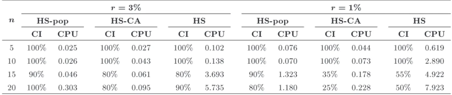
Figure 5. \CPU time-problem size" curve for optimization techniques.
CA, we run these algorithms again for r = 1% and r = 3%. Table 17 shows the results. It can be inferred from Table 17 that although there is no considerable dierence between the CPU times of the two algo-rithms, obviously, HS-pop performs better than HS-CA in convergence. Moreover, the standard HS takes much more CPU time to converge the solution.
We provide the \CPU time-problem size" curve for all optimization techniques. As shown in Figure 5, HS-CA and HS-pop have a better performance than standard HS, and they all perform better than SS and PSO.
8. Conclusion
Due to the existence of competition and market pres-sure, coordinating all entities within a supply chain is
becoming increasingly critical. Some models have been developed to investigate the coordination problem, together with the vendor selection problem. However, little attention has been paid to developing ecient algorithms in this area. By applying the Global Criterion method, the multi-objective mixed integer nonlinear mathematical model is transformed into a single objective optimization problem. Due to the com-plexity of the problem, we propose four metaheuristics: PSO, SS, and two hybrid algorithms, i.e., HS-pop and HS-CA. Then, the comparison is performed among the parameter-tuned algorithms. Solving the sample problems, it is shown that the modied harmony search algorithms (HS-pop and HS-CA) have better perfor-mance than standard HS and they all perform better than SS and PSO in nding high quality solutions in less computational time.
References
1. Thomas, D.J. and Grin, P.M. \Coordinated supply
chain management", Eur. J. Oper. Res., 94(1), pp. 1-15 (1996).
2. Shin, H. and Tunca, T.I. \Do rms invest in forecasting
eciently? The eect of competition on demand
forecast investment and supply chain coordination", Oper. Res., 58, pp. 1592-1610 (2010).
3. Fauli-Oller, R. and Sandonis, J. \Optimal two part
tari licensing contracts with dierentiated goods and endogenous R&D", University of Allicante (2007).
4. Donohue, K.L. \Ecient supply contracts for fashion
goods with forecast updating and two production models", Manag. Sci., 46, pp. 1397-1411 (2000).
coordi-nation with revenue sharing contracts: Strengths and limitations", Manag. Sci., 51, pp. 30-44 (2005).
6. Tsay, A.A. \The quantity exibility contract and
supplier-customer incentives", Manag. Sci., 45, pp. 1339-1358 (1999).
7. Eppen, G.D. and Iyer, A.V. \Backup agreements in
fashion buying - the value of upstream exibility", Manag. Sci., 43, pp. 1469-1484 (1997).
8. Taylor, T.A. \Supply chain coordination under channel rebates with sales eort eects", Manag. Sci., 48, pp. 992-1007 (2002).
9. Li, X. and Wang, Q. \Coordination mechanisms of
supply chain systems", Eur. J. Oper. Res., 179, pp. 1-16 (2007).
10. Sarlak, R. and Nookabadi, A. \Synchronization in
multi-echelon supply chain applying timing discount", Int. J. Adv. Manuf. Technol., 59, pp. 289-297 (2012).
11. Pezeshki, Y., Baboli, A. and Akbari-Jokar, M.R.
\Simultaneous coordination of capacity building and price decisions in a decentralized supply chain", Int. J. Adv. Manuf. Technol., 64, pp. 961-976 (2013).
12. Florez-Lopez, R. \Strategic supplier selection in the added-value perspective: A CI approach", Inf. Sci., 177(5), pp. 1169-1179 (2007).
13. Rosenthal, E.C., Zydiak, J.L. and Chaudhry, S.S.
\Vendor selection with bundling", Dec. Sci., 26, pp. 35-48 (1995).
14. Sarkis, J. and Semple, J.H. \Vendor selection with
bundling: A comment", Dec. Sci., 30(1), pp. 265-271 (1999).
15. Goossens, D.R., Maas, A.J.T., Spieksma, F.C.R. and
Klundert, J.J. \Exact algorithms for procurement problems under a total quantity discount structure", Eur. J. Oper. Res., 178, pp. 603-626 (2007).
16. Ghodsypour, S.H. and O'Brien, C. \A decision
sup-port system for supplier selection using an integrated analytic hierarchy process and linear programming", Int. J. Prod. Econ., 56, pp. 199-212 (1998).
17. Amid, A., Ghodsypour, S.H. and O'Brien, C. \A
weighted additive fuzzy multi-objective model for the supplier selection problem under price breaks in a supply chain", Int. J. Prod. Econ., 121, pp. 323-332 (2009).
18. Jayaraman, V., Srivastava, R. and Benton, W.C.
\Supplier selection and order quantity allocation: A comprehensive model", J. Suppl. Chain Manag., 35, pp. 50-58 (1999).
19. Cakravastia, A., Toha, I.S. and Nakamura, N. \A two-stage model for the design of supply chain network", Int. J. Prod. Econ., 80, pp. 231-248 (2002).
20. Dahel, N.E. \Vendor selection and order quantity
allocation in volume discount environments", Suppl. Chain Manag.: Int. J., 8(4), pp. 335-342 (2003).
21. Xia, W. and Wu, Z.H. \Supplier selection with
multi-ple criteria in volume discount environments", Omega, 35, pp. 494-504 (2007).
22. Ebrahim, R.M., Razmi, J. and Haleh, H. \Scatter
search algorithm for supplier selection and order lot sizing under multiple price discount environment", Adv. Eng. Soft., 40, pp. 766-776 (2009).
23. Herer, Y.T., Rosenblatt, M.J. and Hefter, I. \Fast
algorithms for single-sink xed charge transportation problems with applications to manufacturing and transportation", Transport. Sci., 30(4), pp. 276-290 (1996).
24. Kim, T. and Goyal, S.K. \A consolidated delivery
policy of multiple suppliers for a single buyer", Int. J. Proc. Manag., 2, pp. 267-287 (2009).
25. Kamali, A., Fatemi-Ghomi, S.M.T. and Jolai, F. \A
multi-objective quantity discount and joint optimiza-tion model for coordinaoptimiza-tion of a single-buyer multi-vendor supply chain", Comput. Math. Appl., 62, pp. 3251-3269 (2011).
26. Gheidar-Kjeljani, J., Ghodsypour, S.H. and
Fatemi-Ghomi, S.M.T. \Supply chain optimization policy for a supplier selection problem: a mathematical program-ming approach", Iran. J. Oper. Res., 2(1), pp. 17-31 (2010).
27. Eberhart, R.C. and Kennedy, J. \A new optimizer
using particle swarm theory", In Proceedings of the Sixth International Symposium on Micro Machine and Human Science, Nagoya, Japan, pp. 39-43 (1995).
28. Kennedy, J. and Eberhart, R.C. \Particle swarm
optimization", In IEEE International Conference on Neural Networks, Perth, Australia, pp. 1942-1948 (1995).
29. Glover, F. \Heuristics for integer programming
us-ing surrogate constraints", Dec. Sci., 8, pp. 156-166 (1977).
30. Laguna, M. and Marti, R., Scatter Search:
Method-ology and Implementations, in C. Kluwer Academic Publishers, Boston, MA (2003).
31. Marti, R., Laguna, M. and Glover, F. \Principles of
scatter search", Eur. J. Oper. Res., 169(2), pp. 359-372 (2006).
32. Geem, Z.W., Kim, J.H. and Loganathan, G. \A new
heuristic optimization algorithm: Harmony search", Simulation, 76(2), pp. 60-68 (2001).
33. Mahdavi, M., Fesanghary, M. and Damangir, E. \An
improved harmony search algorithm for solving opti-mization problems", Appl. Math. Comput., 188(2), pp. 1567-1579 (2007).
34. Reynolds, R.G. \An introduction to cultural
algo-rithms", In Proceedings of the 3rd Annual Conference on Evolutionary Programming, World Scientic Pub-lishing, San Diego, Calif, USA, pp. 131-139 (1994).
35. Srinivasan, S. and Ramakrishnan, S. \Cultural
J. Data Mining & Knowledge Manage. Process, 2(5), pp. 53-70 (2012).
36. Sternberg, M. and Reynolds, R.G. \Using cultural
algorithms to support re-engineering of rule based expert systems in dynamic environments: A case study in fraud detection", IEEE Trans. Evol. Comput., 1(4), pp. 225-243 (1997).
37. Gao, X.Z., Wang, X., Jokinen, T., Ovaska, S.J.,
Arkkio, A. and Zenger, K. \A hybrid optimization method for wind generator design", Int. J. Innov. Comput. Inf. Control, 8(6), pp. 4347-4373 (2012). Biographies
Saeed Alaei obtained BS and MS degrees in Industrial Engineering from Amirkabir University of Technology,
Tehran, Iran, in 2009, and Sharif University of Technol-ogy, Tehran, Iran, in 2011, respectively. He is currently a PhD degree candidate in Industrial Engineering at K.N. Toosi University of Technology, Tehran, Iran. His research interests are mainly focused on supply chain coordination, multi-echelon inventory management and game theory.
Farid Khoshalhan received MS and PhD degrees in Industrial Engineering, in 1997 and 2001, respectively, from Tarbiat Modares University, Tehran, Iran. He is currently Assistant Professor in the Faculty of In-dustrial Engineering at K.N. Toosi University of Tech-nology, Tehran, Iran. His research interests include e-commerce and e-business, evolutionary algorithms and metaheuristics, multiple criteria decision making and game theory.