University of Birmingham
Generic probabilistic prototype based classification
of vectorial and proximity data
Schleif, Frank-michael
DOI:
10.1016/j.neucom.2014.12.002 License:
Other (please specify with Rights Statement) Document Version
Peer reviewed version
Citation for published version (Harvard):
Schleif, F 2015, 'Generic probabilistic prototype based classification of vectorial and proximity data', Neurocomputing, vol. 154, pp. 208-216. https://doi.org/10.1016/j.neucom.2014.12.002
Link to publication on Research at Birmingham portal
Publisher Rights Statement:
NOTICE: this is the author’s version of a work that was accepted for publication. Changes resulting from the publishing process, such as peer review, editing, corrections, structural formatting, and other quality control mechanisms may not be reflected in this document. Changes may have been made to this work since it was submitted for publication. A definitive version was subsequently published as Frank-Michael Schleif, Generic probabilistic prototype based classification of vectorial and proximity data, Neurocomputing, http://dx.
doi.org/10.1016/j.neucom.2014.12.002
General rights
Unless a licence is specified above, all rights (including copyright and moral rights) in this document are retained by the authors and/or the copyright holders. The express permission of the copyright holder must be obtained for any use of this material other than for purposes permitted by law.
•Users may freely distribute the URL that is used to identify this publication.
•Users may download and/or print one copy of the publication from the University of Birmingham research portal for the purpose of private study or non-commercial research.
•User may use extracts from the document in line with the concept of ‘fair dealing’ under the Copyright, Designs and Patents Act 1988 (?) •Users may not further distribute the material nor use it for the purposes of commercial gain.
Where a licence is displayed above, please note the terms and conditions of the licence govern your use of this document. When citing, please reference the published version.
Take down policy
While the University of Birmingham exercises care and attention in making items available there are rare occasions when an item has been uploaded in error or has been deemed to be commercially or otherwise sensitive.
If you believe that this is the case for this document, please contact [email protected] providing details and we will remove access to the work immediately and investigate.
Author's Accepted Manuscript
Generic probabilistic prototype based
classi-fication of vectorial and proximity data
Frank-Michael Schleif
PII:
S0925-2312(14)01666-X
DOI:
http://dx.doi.org/10.1016/j.neucom.2014.12.002
Reference:
NEUCOM14955
To appear in:
Neurocomputing
Received date: 15 January 2014
Revised date: 6 September 2014
Accepted date: 3 December 2014
Cite this article as: Frank-Michael Schleif, Generic probabilistic prototype
based classification of vectorial and proximity data,
Neurocomputing,
http://dx.
doi.org/10.1016/j.neucom.2014.12.002
This is a PDF file of an unedited manuscript that has been accepted for
publication. As a service to our customers we are providing this early version of
the manuscript. The manuscript will undergo copyediting, typesetting, and
review of the resulting galley proof before it is published in its final citable form.
Please note that during the production process errors may be discovered which
could affect the content, and all legal disclaimers that apply to the journal
pertain.
Generic probabilistic
prototype based classification
of vectorial and proximity data
Frank-Michael Schleif
School of Computer Science, University of Birmingham, UK
Abstract
In supervised learning probabilistic models are attractive to define discrimi-native models in a rigid mathematical framework. More recently, prototype approaches, known for compact and efficient models, were defined in a proba-bilistic setting, but are limited to metric vectorial spaces. Here we propose a generalization of the discriminative probabilistic prototype learning algorithm for arbitrary proximity data, widely applicable to a multitude of data analy-sis tasks. We extend the algorithm to incorporate adaptive distance measures, kernels and non-metric proximities in a full probabilistic framework.
1. Introduction
Discriminative models are of wide interest but few provide probabilistic out-puts while being applicable fornon-vectorial data. Modern measurement tech-nologies in the life sciences, but also in the field of social interaction, provide large sets of similarities or dissimilarities between the data, but without an un-derlying vector space [1]. Examples are scores of sequence data and proximities, occurring in social networks, but often also vectorial data are represented by proximities, for example by the use of kernel functions.
The data can be represented byN×N matrices of proximity measures, with
N as the number of samples. As discussed in [1] embedding approaches can be used to apply vector space models, but these are costly with typicallyO(N3)
complexity. In case of similarities, standard inner-product approaches, or kernel methods [2] can be used, with the assumption of an underlying metric space.
For dissimilarity data novel prototype classifier algorithms have been pro-posed recently in [3], focusing on crisp classification decisions. Only few prob-abilistic classifiers for proximity data are available, like the probprob-abilistic classi-fication vector machine [4] for similarity data or the approach published in [3]. Here we present an approach which is applicable for vectorial and non-vectorial representations and can also be applied to non-metric data, by an implicit pre-processing of the proximity matrix.
2 PROTOTYPE BASED LEARNING 2
Prototype-based methods are of special interest, because they represent their decisions in terms of typical representatives, contained in the input space, or by approximations thereof. Prototypes can directly be inspected by human experts similar as data points: for example, physicians can inspect prototypical medi-cal cases [5, 6], prototypimedi-cal images can directly be displayed on the computer screen, prototypical action sequences of robots can be performed in a robotic simulation, etc. Since the decision in prototype-based techniques usually de-pends on the similarity of a given input to the prototypes stored in the model, a direct inspection of the taken decision in terms of the responsible prototype becomes possible. A probabilistic output provides additional value to judge the reliability of the model decision.
Many different algorithms have been proposed in the literature, which derive discriminative prototype based models from given data, see e.g. [7, 8, 9, 10, 11], but only few support probabilistic outputs [8], still being inherently genera-tive. In [12] a fully probabilistic prototype model was derived for vectorial data, closely related to earlier work of the authors [13], where the so called Multi-variate class labeling soft robust learning vector quantization (MRSLVQ) was proposed. In addition to their direct interpretability [14], prototype-based mod-els provide excellent generalization ability, due to their sparse representation of data, see e.g. the work [15, 16] for explicit large margin generalization bounds. The task of supervised classification of proximities occurs in diverse com-plex applications, such as the classification of mass spectra according to the biomedical decision problem [17, 18] or the classification of music according to underlying composers or epochs [19]. Supervised prototype-based techniques for general dissimilarity data would offer one striking possibility to arrive at human understandable classifiers in such settings.
In this contribution, we shortly review discriminative probabilistic learning (DPL) as recently proposed in [12] and extend it, such that parametric distances and proximity data can be used. We will call this approach generalized DPL (GDPL). Additionally we address the problem of non-metric proximities and how these can be corrected to be used in GDPL. We also address the processing of soft labeled data sets in the context of DPL and GDPL not directly considered in the original proposal of DPL. Experimental results at synthetic and real life data confirm the efficiency of our approach.
2. Prototype based learning
Assume data xi ∈ RD, i = 1, . . . , N, are given in a D dimensional space.
Prototypes are elementswj ∈RD, j = 1, . . . , K, of the same space withW =
{w1, . . . ,wK}, the set of all prototypes of the model. They decompose the data
into receptive fields
R(wj) ={xi : ∀k d(xi,wj)≤d(xi,wk)}
based on a metric distance measure, like the squared Euclidean distance
3 DISCRIMINATIVE PROBABILISTIC LEARNING 3
We further define the short-cutdj for Eq 1 with respect to thej-th prototype,
and the index i of the point xi will be clear from the context. The goal of
prototype-based machine learning techniques is to find prototypes which repre-sent a given data set as accurately as possible. We will also assume that the data
xiare equipped with prior class labelsc(xi)∈ {1, . . . , L}in a finite set of given
classes in the crisp case or can be associated to a vector of class assignments
l(xi)∈ [0,1]L, normalized such thatP L
k l(xi)k = 1, which we will call soft or
fuzzy labels.
Supervised prototype based modeling is established on two concepts, first the data are represented by means of a representer concept, e.g a Gaussian distribution [8], a mixture of Gaussians [12], a topographic model [20] or other types of data representations which can be considered as the quantization step where larger sets of data are summarized by a smaller number of prototypes and the data itself are subsequently analyzed, based on the derived compact representation.
In the second step these representations can be used e.g. to derive a clas-sification model, which can again be based on different concepts as likelihood ratios [8], inner-class constraints [7] or a softmax classifier [12], as it will be used in the following. Typically both steps are linked to each other and the parame-ters are optimized based on a cost function, using some optimization strategy, like gradient descend, quasi-newton optimization or others. If thexi are given
in a vectorial space as defined before, standard techniques like the Generalized Learning Vector Quantizer (GLVQ) [7] can be used to obtain the prototype models and a classifier model can be defined, see [7] for a detailed derivation. As mentioned before few prototypes models are based on a probabilistic model, the most are inherently generative, rather then purely probabilistic. An excep-tion is the multilabled robust soft LVQ (MRSLVQ) [13] and DPL [12], both very similar. We will now review the main concepts of DPL and extend it in different ways.
3. Discriminative probabilistic learning
3.1. Data representation
In the original DPL formulation a given pointxiis defined as aset of multiple
feature vectors of the same dimension, accordingly a point is given as vi =
{qi,1, . . . ,qi,Qi}withQi as the number of feature vectors of pointviandqi,·∈
RD. Such a setting occurs e.g. in image analysis where an image i can be
represented as a number of potentially overlapping patches withDentries each. The number of feature vectorsQi can be different for each point vi. IfQi = 1
we have a standard vector quantization problem where a point can be directly associated to a number of features. The representation of the data, during the optimization, is modeled by a functionr(q), which in case of typical prototype learners like LVQ is given in a winner takes all scheme:
rj(q, W) =||wj−q||2·
(
1 if||wj−q||2≤ ||wj0−q||2 ∀j06=j
3 DISCRIMINATIVE PROBABILISTIC LEARNING 4
Here a feature vectorq is represented by the distance to its closest prototype
wj, an alternative is to use a measure of responsibility as it was done in [13] as
well as in DPL: rj(q, W, β) = exp(−β||wj−q||2) PK j0 exp(−β||wj0 −q||2) = exp(−βd(wj,q)) PK j0 exp(−βd(wj0,q)) (3)
Here the feature vector is not necessarily assigned to a single prototype but each prototype is responsible for it to some degree in a probabilistic manner andβis the inverse variance of the Gaussian. To cope with multiple feature vectors for a single point in DPL the representation of a pointviwith respect to a prototype
wj is given e.g. as zj(vi, W, β) = Qi X s=1 πirj(qi,s, W, β) (4)
withπi being a normalizer typically set toπi= Q1i. The latent representation
of a point v will be given accordingly as a vector z = [z1(v), . . . , zK(v)]>,
whereKis again the number of prototypes. Using this notation a pointviwith
multiple feature vectorsqi,·is represented by multiple prototypes, summarizing
similar feature vectors over multiple points vi. The latent points form a set
Z={z1, . . . ,zN}, As the second step a classifier function is defined usingzas
input. Such a classifier can be based on the GLVQ cost function using winner takes all in the final classification decision or a probabilistic classifier as used in DPL.
3.2. Soft max classification and optimization
DPL takes a softmax classifier on top of the data representation approach such that: P(li=c|z) = exp(θ> c z) PL c0=1exp(θc>0z) =σc(z; Θ) (5)
where Θ ={θ1, . . . , θL}withθc∈RK, ∀kPLc Θk,c = 1. The matrix Θ contains
the soft labels of the prototypes. In the following we may skip parameters of a function if they are known from the context.
Assuming the data are i.i.d., the log-likelihood of the data can be modeled as L(Θ, β, W) = N X i ˆ P(li)·logP(li=c|zi(vi, W, β),Θ) (6)
where ˆP(li) refers to the soft label of the datapointi. Now this likelihood is
4 RELEVANCE LEARNING 5
Using (3) as a representation model, the necessary gradients for the parameters are given as:
∂L ∂wd j = N X i K X j0 ∂zji ∂wd j0 ·∂Li ∂zji (7) andi= 1, . . . , N,j, j0= 1, . . . , K andd= 1, . . . , D. ∂zji ∂wd j0 = Qi X s=1 rj(qi,s) = βPQi s=1rj(qi,s)·(1−rj(qi,s))· ∂dj ∂wd j0 ⇐⇒ j=j0 βPQi s=1rj(qi,s)·rj0(qi,s))· ∂dj ∂wd j0 where ∂dj ∂wd j
is the derivative of the representation function to its parameters, here in general a derivative of a standard distance measure with respect towd j
is used. For the parameterβ we get:
∂L ∂β = N X i K X j ∂zji ∂β · ∂Li ∂zji (8) with ∂zji ∂β = Qi X s=1 rj(qi,s) K X j0=1 rj0(qi,s)dj0−dj (9)
The derivative with respect to the latent representationz used above is given as: ∂L ∂zji = L X c ˆ P(li)=c−σc(zji; Θ))·θc (10)
With ˆP(li)=cbeing the value at the index referring to classcof the soft label of
data pointi. For the gradient with respect to the soft labels, used as parameters of the classifiers, we get
∂L ∂θc = N X i=1 ( ˆP(li)=c−σc(zi; Θ))·zi (11) 4. Relevance learning
The principle of relevance learning has been introduced in [21, 22] with generalizations in [23] as a particularly simple and efficient method to adapt the
4 RELEVANCE LEARNING 6
underlying metric of prototype based classifiers according to the given situation at hand using available auxiliary information. It takes into account a relevance scheme of the data dimensions by substituting the squared Euclidean metric by the weighted form
dλ(q,w) =
D
X
d=1
λ2d(qd−wd)2. (12)
whereqdrefers to the dimensiondof the feature vectorqwhich belongs to some
pointv. The principle is extended in [24] to the more general metric form
dΩ(x,w) = (q−wT)ΩTΩ
| {z }
Λ
(q−w) (13)
Using a squared matrixΩ, a positive semi-definite matrix which gives rise to a valid pseudo-metric is achieved this way. In [24], these metrics are considered in local and global form, i.e. the adaptive metric parameters can be identical for the full model, or they can be attached to every prototype present in the model [25]. As proposed in [26] the form given in (13) can also be used with limited ranks such that the matrix Ω needs not to be of squared form Ω ∈ RM×N,
withM ≤N. Using M = 2,3 a low dimensional projection matrix of the data is obtained which incorporates the auxiliary label information of the training and provides a discriminative mapping. A specific discussion of the approach including a theoretical analysis is given in [26]. In [11] matrix learning has also been addressed in the DPL context. The derivatives of the distance used in the previous section with respect to this parametrized metric, using matrix notation, is given as:
∂dj
∂w = −2Ω
>Ω(w
j−q) (14)
The optimization of the matrix parameters, assuming a global matrix, is given as ∂L ∂Ωm,n = N X i K X j ∂zji ∂Ωm,n ·∂Li ∂zji (15) ∂zji ∂Ωm,n = Qi X s=1 rj(qi,s) K X j0=1 r0j(qi,s) ∂d0j ∂Ωm,n − ∂dj ∂Ωm,n (16) ∂dj ∂Ωm,n = 2[Ω(wj−q)]m·(wj,n−qn) (17)
The updates for the diagonal matrixλor local matrix formulations per class or per prototype are derived directly as a special case from equation (15). After each update step the distance parameters are adapted to fulfill
X i λi,i= X m,n Ω2m,n= 1
5 PROXIMITY DATA 7 x -2.5 -2 -1.5 -1 -0.5 0 0.5 1 1.5 2 2.5 y -2.5 -2 -1.5 -1 -0.5 0 0.5 1 1.5 2 2.5 x -2.5 -2 -1.5 -1 -0.5 0 0.5 1 1.5 2 2.5 y -2.5 -2 -1.5 -1 -0.5 0 0.5 1 1.5 2 2.5
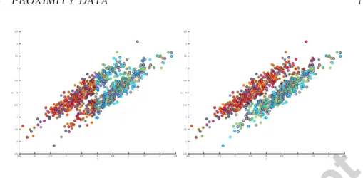
Figure 1: Relevance (left) vs matrix (right) relevance learning for a simulated ellipsoid dataset. The color shades indicate the classification uncertainty. For the relevance DPL we observe clear miss-classification because the receptive field is aligned to one of the input axes, whereas for matrix learning the receptive fields are diagonal, following the data distribution.
Further details can be found in [26, 24, 27]. In Figure 1 we show the results of matrix relevance learning in DPL for a simulated dataset of two two-dimensional ellipsoids which are not linear separable using classical Euclidean relevance learning where only the relevance of individual input dimensions but not the correlation thereof can be weighted. We use 1 prototype per class and do a five-fold crossvalidation. The mean test set error using classical relevance learning is 23.5±1.9 and for matrix relevance learning one achieves 2.60±2.77.
5. Proximity data
Prototype-based techniques as introduced above are restricted to Euclidean vector spaces such that their suitability to deal with complex non-vectorial data sets is highly limited. In the following, we assume that data pointsx or vare not given as vectors, but in form ofpairwise proximities. These proximities are measures of the relatedness of pairs of points. Considering e.g. sequence data, such a proximity value can be calculated by using popular alignment algorithms [28]. Often such values occur in form of similarities, with more similar objects having higher values and highest values for self similarities.
To obtain a valid probabilistic model we assume that the proximities are metric. In case of non-metric data corrections on the, potentially approximated matrix, can be applied as shown in [29, 30]. Metric similarities can be considered to be inner products forming a valid kernel. As shown in [3], prototype based learning algorithms can be reformulated to support kernels instead of vector data, either using batch approaches [31] or in the online settings [32]. Also approaches for dissimilarities have been proposed recently [3].
In the following we will give a formulation of DPL for metric dissimilarity data without an explicit underlying vector space. Kernels can be used as a special case of this formulation using the following equation to obtain squared
5 PROXIMITY DATA 8
distances based on given inner products
d(w,x) =hx,xi+hw,wi −2· hx,wi
Assume dissimilaritiesdi,j =d(xi,xj) of data points numberediand j are
available. D ∈ RN×N refers to the corresponding dissimilarity matrix. Note
that it is easily possible to transfer similarities to dissimilarities and vice versa, see [29]. To obtain a valid probabilistic model we assumeDto be metric, which can be achieved using approaches discussed in [29, 30].
Since the embedding of the data in a vector space is usually not given ex-plicitly and computation of an explicit embedding takes cubic complexity, the prototypes are usually adapted only implicitly based on the following observa-tions: assume prototypes are represented as linear combinations of data points
wj= X i αjixi with X i αji= 1.
Then dissimilarities can be computed implicitly by means of the formula
d(xi,wj) =kxi−wjk2= [D·αj]i−
1 2 ·α
t
jDαj
where αj = (αj1, . . . , αjn) refers to the vector of coefficients describing the
prototypewj implicitly.
This way, model adaptation of DPL in a pseudo-Euclidean space can be per-formed implicitly. This way, prototypes are represented implicitly by means of their coefficient vectors, and adaptation refers to the know pairwise dissimilar-itiesdij only. We refer to this approach as the relational DPL (RDPL) in the
following. Initialization takes place by setting the coefficients to random vectors which sum up to 1. Even for general settings, this assumption is quite reason-able since we can expect that the prototypes lie in the vector space spanned by the data.
This implicit distance calculation can be used in the log-likelihood function of DPL, replacing the standard Euclidean distance given in (3) by the appro-priate (parametric) distance measure. The update equations forβ are adapted accordingly. The update of parameter w is replaced by updates for the pa-rameterα. Theαparameters can be summarized in the matrix Γ with entries
α∈RK×N. The rows of this matrix represent the coefficients of a prototype,
normalized as discussed above. Note that the number of columns of Γ need not to beN, but this representation set can be limited to fewer coefficients, using random sampling or sparsity approaches [33, 34].
A componentkof theseαvectors is adapted by the rules
∂[Dαj]i−12·α t jDαj ∂αjk = dK− X l dlkαjl
After every adaptation step, normalization takes place to guaranteeP
iαji= 1.
6 EXPERIMENTS 9
similar to DPL is given for general dissimilarity data, whereby prototypes are implicitly embedded in the pseudo-Euclidean space.
The prototypes are initialized as random vectors, i.e we initialize αij with
small random values such that the sum is one. It is possible to take class information into account by setting allαij to zero which do not correspond to
the class of the prototype.
The resulting classifier represents clusters in terms of prototypes for general dissimilarity data. Although these prototypes correspond to vector positions in pseudo-Euclidean space, they can usually not be inspected directly because the pseudo-Euclidean embedding is not computed directly. Therefore, we use an approximation of the prototypes after training, substituting a prototype by its
Knearest data points as measured by the given dissimilarity. To achieve a fast computation of this approximation, we enforceαij ≥0 during the updates.
Note that generalization of the classification to new data can be easily done given a novel data point x characterized by its pairwise dissimilarities D(x) to the data used for training, the dissimilarity to the prototypes is given by
d(x,wj) = D(x)t·αj − 12 ·αtjDαj. For an approximation of prototypes by
exemplars, obviously, only the dissimilarities to these exemplars have to be computed, i.e. a very sparse classifier results. The memory and runtime com-plexity can be further reduced by using approximation concepts for low rank matrices of the proximity matrices as recently discussed in [35, 29, 36].
6. Experiments
We evaluate the generalized DPL algorithm for different vectorial datasets, employing the parametrized distance and a relational distance measure using multiple public data sets. We also address how to interpret the probabilistic prototype models for the different types of input formats.
6.1. Vectorial data
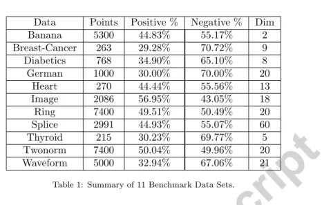
In this section we evaluate the efficiency of the proposed approach on a large set of vectorial data. We use the Raetsch benchmark data [37], which are widely based on datasets provided in the UCI machine learning repository [38] but with given splits in a 100 fold crossvalidation. Data characteristics are given in Table 1
In [39] also a scheme for the estimation of meta parameters is provided which we use to estimate the number of prototypes or, later on, the sigma parameter of the used rbf-kernel. Here we use only those datasets from [37] which contain at least 150 points.
We evaluate GDPL with a parametric metric as shown before defined as matrix learning. This strategy permits a linear transformation of the input data with respect to the most discriminating features and correlations thereof. As shown before [9] this approach is often very effective also to prune out irrelevant or noisy data dimensions, however it does not help in case of non-linear separable problems, where kernel methods are more appropriate. The standard DPL,
6 EXPERIMENTS 10
Data Points Positive % Negative % Dim Banana 5300 44.83% 55.17% 2 Breast-Cancer 263 29.28% 70.72% 9 Diabetics 768 34.90% 65.10% 8 German 1000 30.00% 70.00% 20 Heart 270 44.44% 55.56% 13 Image 2086 56.95% 43.05% 18 Ring 7400 49.51% 50.49% 20 Splice 2991 44.93% 55.07% 60 Thyroid 215 30.23% 69.77% 5 Twonorm 7400 50.04% 49.96% 20 Waveform 5000 32.94% 67.06% 21
Table 1: Summary of 11 Benchmark Data Sets.
potentially improved by a parametric distance can handle such complicated decision boundaries only to some degree, by adjusting the number of prototypes. The number of prototypes per class has been optimized using a grid search of 1−10 prototypes per class. We will call this approach DPL-Matrix in the following.
As known from previous work, kernels can often provide simple solutions for non-linear decision problems. Accordingly, we evaluate GDPL also by using an RBF kernel, with an optimized sigma. The sigma was optimized again by a grid search on sigma values in [0.1,10]. We will call this approach DPL-RBF in the following.
We compare our results with recently published results on the same data sets using the Probabilistic Classification Vector Machine (PCVM) [4] and the best results of the support vector machine (SVM) [40] taken from [4]. The PCVM is a probabilistic classifier for two class decision problems, applicable for positive definite similarity matrices. We used an RBF kernel with an optimized sigma.
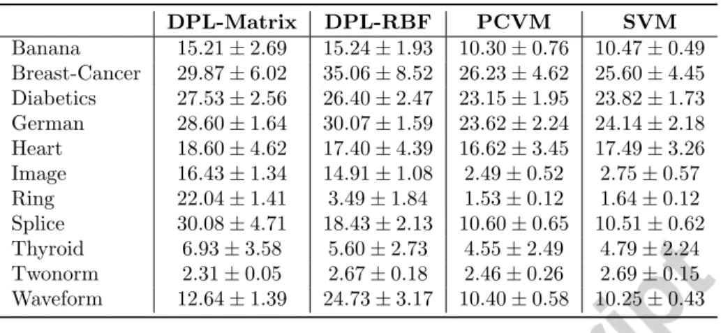
PCVM, SVM as well as DPL-RBF are able to define non-linear decision boundaries and should be efficient to model non-linear decision problems. The corresponding results are shown in Table 2.
From the comparison in Table 2 we observe that the DPL-Matrix approach is in general slightly worse than the other approaches. This is mainly due to the non-linearities in the considered datasets, which were originally proposed and selected to evaluate kernel methods. Using a kernel matrix in DPL it is consistently better compared with DPL-Matrix and most often competitive with the results of PCVM or SVM. For the DPL-RBF results we used only one prototype per class, such that the model complexity is comparable with PCVM. DPL and GDPL permits however to adapt the number of prototypes such that also the aspect of multi modality in the data can be easier addressed.
6 EXPERIMENTS 11 DPL-Matrix DPL-RBF PCVM SVM Banana 15.21±2.69 15.24±1.93 10.30±0.76 10.47±0.49 Breast-Cancer 29.87±6.02 35.06±8.52 26.23±4.62 25.60±4.45 Diabetics 27.53±2.56 26.40±2.47 23.15±1.95 23.82±1.73 German 28.60±1.64 30.07±1.59 23.62±2.24 24.14±2.18 Heart 18.60±4.62 17.40±4.39 16.62±3.45 17.49±3.26 Image 16.43±1.34 14.91±1.08 2.49±0.52 2.75±0.57 Ring 22.04±1.41 3.49±1.84 1.53±0.12 1.64±0.12 Splice 30.08±4.71 18.43±2.13 10.60±0.65 10.51±0.62 Thyroid 6.93±3.58 5.60±2.73 4.55±2.49 4.79±2.24 Twonorm 2.31±0.05 2.67±0.18 2.46±0.26 2.69±0.15 Waveform 12.64±1.39 24.73±3.17 10.40±0.58 10.25±0.43
Table 2: Experimental results (test set errors) for the raetsch benchmark data using DPL with a parametric distance (DPL-Matrix) and an rbf kernel (DPL-RBF) in comparison to state of the art results using PCVM and SVM, both also with an RBF kernel.
6.1.1. Interpretation of prototypes
Using the parametric distance in DPL we are able to analyze the discrimina-tion properties of individual or correlated input features of the data. As already shown previously in [24, 6] for other prototype based learning algorithms, this is often a key element to obtain effective decision models in a way, such that the decision function remains interpretable and can be communicated to an expert. Often it is alsonecessary to limit the number of input features to permit easier technical implementations [41], which is not so easy by use of kernel approaches. For kernel methods the identification of discriminating features in the original input data is complicated due to the highly non-linear decision function, in-troduced by the kernel-mapping and only few approaches have been proposed so far, focusing most often on linear kernels or using complex calculations and wrappers for non-linear kernel functions [42].
In Figure 2, exemplary so called relevance profiles and matrices as obtained from DPL-matrix, for a sample dataset, are shown. The relevance profile shows the calculated weighting of each features used in the distance calculations, as obtained during the optimization process. High weights indicate features which discriminate well between the classes whereas low ranked features are either non- or less discriminative, or redundant. Using this approach unimportant features can be effectively pruned out of the model, which can be helpful in post analysis or technical processing steps of the data. The relevance matrix is helpful to show the correlation of different features. This can be beneficial to obtain a better understanding of the interaction of measurement variables, e.g. for different sensor channels.
6 EXPERIMENTS 12
Training Points DPL-Matrix DPL-RBF PCVM SVM
Banana 400 14 71.4±2.79 19.8±4.3 111.1±8.9 Breast-Cancer 200 18 16.6±4.82 9.4±2.6 125.2±6.25 Diabetics 468 2 37±1.41 19.8±3.1 265.0±7.0 German 700 18 18±1.22 40.9±7.6 520.9±10.9 Heart 170 14 15.2±0.83 5.9±2.2 103.7±5.3 Image 1300 20 108±3.74 170.3±11.7 396.9±11.4 Ring 400 16 50±0.71 17.6±3.8 198.6±10.8 Splice 1000 4 65.4±1.67 123.2±8.3 778.8±13.6 Thyroid 140 8 73±2.35 8.6±2.3 24.8±3.7 Twonorm 400 2 14.8±0.45 13.8±3.4 237.4±7.1 Waveform 400 10 76.2±11.92 26.3±3.7 229.6±8.8
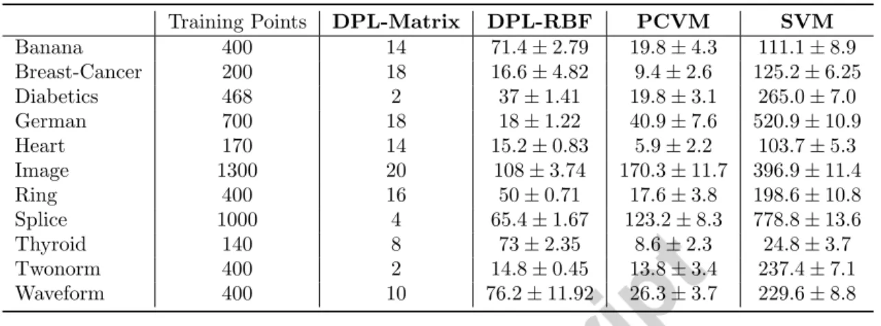
Table 3: Overall modelcomplexity on 100 runs on the raetsch test data. For DPL-RBF we report the mean/std of the number of points necessary to represent the prototypes. The results for PCVM and SVM are taken from [4].
1 2 3 4 5 6 7 8 9 0 0.05 0.1 0.15 0.2 0.25 Feature Relevance Feature Feature 1 2 3 4 5 6 7 8 9 1 2 3 4 5 6 7 8 9 −0.1 −0.08 −0.06 −0.04 −0.02 0 0.02 0.04 0.06
Figure 2: Relevance profile of breast cancer data (left). Corresponding Λ matrix showing the correlation between the variable. We observe features with high relevances e.g. 3,6,7. Some features are correlated or anti-correlated, see e.g. feature 5 and 6.
6.2. Proximity data
The processing of similarity matrices is relevant, because many machine learning algorithms are based on kernels and take the similarity between ob-ject as inputs. Here we evaluate the relational DPL for seven benchmark data sets where data are characterized by pairwise dissimilarities and which have been preprocessed by flipping using strategies discussed in [29] to obtain metric dissimilarities. We also compare our findings with an alternative probabilistic kernel classifier (PCVM) provided in [4] and a standard core-vector machine (CVM) implementation [43].
1. Protein: 213 proteins are compared based on evolutionary distances com-prising four different classes according to different globin families. Label-ing is given by four classes correspondLabel-ing to globin families.
2. The Copenhagen chromosomes data set constitutes a benchmark from cy-togenetics [44]. A set of 4,200 human chromosomes from 22 classes (the au-tosomal chromosomes) are represented by grey-valued images. These are
6 EXPERIMENTS 13
transferred to strings measuring the thickness of their silhouettes. These strings are compared using edit distance with insertion/deletion costs 4.5 [28].
3. The proteom dissimilarity data set [45] with 2604 samples in 53 imbalanced classes
4. The Delft gestures data with 1500 samples in 20 balanced classes taken from [45]. The dissimilarities are generated from a sign-language interpre-tation problem with 1500 samples in 20 classes and 75 samples per class. The gestures are measured by two video cameras observing the positions of the two hands in 75 repetitions of creating 20 different signs. The dis-similarities are computed using a dynamic time warping procedure on the sequence of positions [46].
5. The Zongker digit dissimilarity data consisting of 2000 samples in 10 bal-anced classes taken from [45]. This dataset is based on deformable tem-plate matching. The dissimilarity measure was computed between 2000 handwritten NIST digits in 10 classes, with 200 entries each, as a result of an iterative optimization of the non-linear deformation of the grid [47] 6. The Voting data set comes from the UCI Repository [38]. It is a two-class two-classification problem with 435 samples, where each sample is a cat-egorical feature vector with 16 components and three possibilities for each component a value difference metric was computed from the categorical data, which is a dissimilarity that uses the training class labels to weight different components differently so as to achieve maximum probability of class separation.
7. The Aural Sonar data set is from a recent paper which investigated the human ability to distinguish different types of sonar signals by ear. The signals were returns from a broadband active sonar system, with 50 target-of-interest signals and 50 clutter signals. Every pair of signals was assigned a similarity score from 1 to 5 by two randomly chosen human subjects unaware of the true labels, and these scores were added to produce a 100×100 similarity matrix with integer values from 2 to 10 [48].
These seven data sets constitute typical examples of non-Euclidean data which occur in complex systems, such as medical image analysis and symbolic domains. In all cases, dedicated preprocessing steps and dissimilarity measures for struc-tures were used to generate the data. The dissimilarity measures are inherently non-Euclidean and have been corrected using the approaches discussed in [29].
We report the results of generalized DPL in comparison to different alter-natives for these data sets. The number of prototypes is picked according to the number of given classes. The prototypes are initialized either in the center of corresponding classes (vectorial case), or using a classwise initialization of the alphas, with additive random noise. Training is done using quasi newton optimization until convergence with an upper limit of 100 steps.
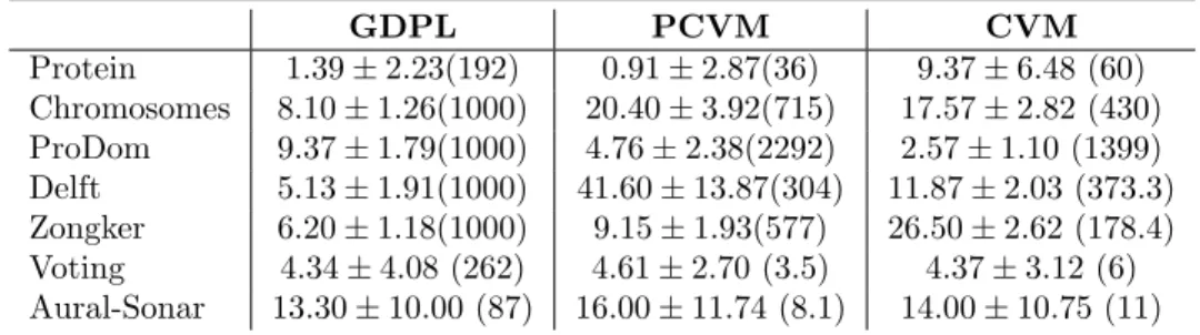
The results are evaluated by the classification accuracy on the test set ob-tained in a repeated stratified 10-fold cross-validation with 10 repeats. The results are reported in Tab. 4.
7 DATA WITH UNCERTAIN LABEL INFORMATION 14 GDPL PCVM CVM Protein 1.39±2.23(192) 0.91±2.87(36) 9.37±6.48 (60) Chromosomes 8.10±1.26(1000) 20.40±3.92(715) 17.57±2.82 (430) ProDom 9.37±1.79(1000) 4.76±2.38(2292) 2.57±1.10 (1399) Delft 5.13±1.91(1000) 41.60±13.87(304) 11.87±2.03 (373.3) Zongker 6.20±1.18(1000) 9.15±1.93(577) 26.50±2.62 (178.4) Voting 4.34±4.08 (262) 4.61±2.70 (3.5) 4.37±3.12 (6) Aural-Sonar 13.30±10.00 (87) 16.00±11.74 (8.1) 14.00±10.75 (11)
Table 4: Crossvalidation errors of GDPL for proximity data, where no underlying vector space exists. Non-metric proximities have been corrected using the flip approach (see text) as a necessary pre-processing to obey valid probabilistic models and a psd kernel. The model complexity by means of training points used in the model is given in parenthesis.
The results show that the CVM model is very effective in learning the given classification problems, given the proximity matrices have been adapted by an eigenvalue correction beforehand. Analyzing the number of support vectors we observe, that the models of PCVM and GDPL are less effective, which is mainly caused by the very sparse underlying modeling, using a prototype concept. The PCVM uses truncated Gaussians for each point, which are sparsified during learning and the GDPL uses a single Gaussian to approximate a whole class. While PCVM scales the model complexity in a self-adaptive process, GDPL has no such mechanism, but we could estimate the number of prototypes as a meta parameter using the same scheme as before or by using adaptation concepts as recently proposed in [49]. Here we simply used 1 prototype for class for the Protein data and 10 prototypes per class for the remaining data sets. The number of representation points was fixed to a maximal number of 1000 selected randomly fromN. The corresponding results are shown in Table 4.
7. Data with uncertain label information
In the former sections we considered data which have been labeled by crisp labels, such that the assignment of a data point to a class is unique. For mul-tiple data sets e.g. in the life sciences the assumption of given crisp labels is unrealistic. In medicine a patient can be classified to a specific type of disease, but this decision is often based on multiple measurements, all of which having an individual errors and the decision is frequently based on measures mapped to intervals, which can not be defined in a definite manner. Other prominent examples can be found e.g. for sensor systems, where the sensor has a limited resolution and the acquired signal is effectively a mixture of different substances. This is probably most obvious in remote sensing, where the spatial resolution is in the range of some square meters but for each pixel often a unique substance class is assigned. Accordingly, labelings are often not unique. Beside of classical Bayesian models only few machine learning methods can deal with uncertain input label information. The formerly mentioned PCVM provides probabilistic
7 DATA WITH UNCERTAIN LABEL INFORMATION 15
outputs, but the input label of a point has to be 0/1 or -1 / 1 respectively. Also many other prominent classifier algorithms are limited to crisp labels like the SVM or CVM. The DPL and the MRSLVQ approach can deal with uncertain input labels. In the following we give experimental results for artificial and real life data with uncertain labels and show the benefits of the inclusion of this information in the modeling process. While the original DPL and MRSLVQ formulation are already useful for uncertainly labeled data we are now also able not only to use a linear representation of the data sets but can also employ a ker-nel encoding to simplify the modeling process and to improve the generalization capabilities.
The following datasets have been analyzed
1. The synthetic data (Gaussian) is based on two Gaussians in 2Dwhich are slightly overlapping. From these two distributions 1000 points are drawn randomly and mixed with some probability. The mixing probabilities define the uncertain labeling. A sample of the data is shown in Figure 3. 2. Plant tissue data The data are 4418 points of 22 dimensional image fea-tures in 11 classes of a serial transverse section of barley grains taken from [50]. Developing barley grains consist of three genetically different tissue types: the diploid maternal tissues, the filial triploid endosperm, and the diploid embryo which are hard to distinguish. This data was originally provided with crisp and fuzzy labels.
3. Remote sensing data is a multi-spectral LANDSAT TM satellite image of the Colorado area taken from [51] with 6 different spectral bands. The LANDSAT TM bands were strategically determined for optimal detec-tion and discriminadetec-tion of vegetadetec-tion, water, rock formadetec-tions and cultural features. There are 14 labels describing different vegetation types and ge-ological formations. The size of the original image is 1907×1784 pixels1. Fuzzy labels where obtained by a downsampling of this data set to 12650 points where the original image was cut to 1760×1840 pixel2. The fuzzy
labels were derived from the histograms of the averaged pixel areas. The model complexity for PCVM is adapted automatically whereas for DPL we need to provide the number of prototypes, as mentioned before. For the Gaussian and the Plant-Tissue data we use 1 prototype per class and for the Remote-Sensing data we use 10 prototypes per class, as suggested in former work with the original remote sensing data set [51].
The results are shown in Table 5 and Figure 3. For the synthetic data shown in Figure 3 we observe a clear change in the decision boundary. The DPL model, which is capable to account for fuzziness in the input label reflects the uncer-tainty about the data labeling in a corresponding large uncertain prediction area. For the PCVM model the uncertain region is small because the addi-tional information about uncertain input labels can not be used in the modeling
1Thereby 9 pixel have an unknown label and have been removed. 2Here we just cut the right and lower boundary of the image
7 DATA WITH UNCERTAIN LABEL INFORMATION 16 −3 −2 −1 0 1 2 3 4 −4 −3 −2 −1 0 1 2 3 4 Synthetic data (a) a −3 −2 −1 0 1 2 3 4 −4 −3 −2 −1 0 1 2 3 4
DPLVQ model with crisp label inputs and contour lines
(b) b −3 −2 −1 0 1 2 3 4 −4 −3 −2 −1 0 1 2 3 4
DPLVQ model with soft label inputs and contour lines
(c) c −3 −2 −1 0 1 2 3 4 −4 −3 −2 −1 0 1 2 3 4
PCVM model with crisp label inputs and contour lines
(d) d
Figure 3: Synthetic data set to illustrate uncertain labelings. Plot a) shows 1000 sample points mixed from two Gaussian distributions. Plot b) shows the predicted label of a linear DPL model with crisp labels as input. Plot c) shows the predicted labels with DPL having soft labels as input. Plot d) shows the predicted label using PCVM and crisp labels. All models have a similar accuracy of≈ 84%, but the mean square label error (MSLE) is three times smaller using DPL with soft label inputs compared to DPL or PCVM with crisp inputs. We see that DPL+Crisp and PCVM behave similar but the area of (indeed) uncertain points is much larger for DPL using soft labels as inputs. The contours with respect to class 1 (squares in red) are given as 0.25 (red), 0.5 (cyan) and 0.75 (green). Probabilistic labels are given by different color shades (bright is safer), the shape indicates the predicted crisp class label.
8 CONCLUSIONS 17
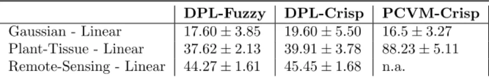
DPL-Fuzzy DPL-Crisp PCVM-Crisp
Gaussian - Linear 17.60±3.85 19.60±5.50 16.5±3.27 Plant-Tissue - Linear 37.62±2.13 39.91±3.78 88.23±5.11 Remote-Sensing - Linear 44.27±1.61 45.45±1.68 n.a.
Table 5: Crossvalidation errors of the uncertainly labeled data. We show the mean and standard deviation of the test error where the labeling of the points and model outputs has been taken as a crisp label or fuzzy labels depending on the algorithm-properties. For the PCVM model the remote sensing data failed to converge.
step. Also in the Table 5 we observe improved prediction accuracies for the DPL-Fuzzy model compared to its crisp counterpart, when the data are fuzzy labeled. In comparison to the PCVM model we observed slightly better results for the simulated Gaussian data, but for the other datasets a substantially worse performance was found. The real data sets are obviously very challenging for PCVM, likely due to the strong overlaps of the different classes. The information provided by the uncertain labeling is not available to PCVM and accordingly it is hard to estimate the underlying class distribution. Also DPL is less effective if only crisp labels are given but this effect is not so strong.
8. Conclusions
In this article we presented multiple extension of Discriminative Probabilis-tic LVQ to support adaptive relevance learning and the analysis of proximity matrices in the form of kernel or dissimilarity matrix data. We compared the proposed method with state of the art approaches on a number of test data. In the first experiments (see Table 2) we observed that the extensions of DPL are very effective, leading to competitive results for those data which are known to be linear separable. Here we have also shown how to analyze the most relevant discriminating features from the model a property which is of wider interest and often not directly available in many methods. For those data which are non-linear separable we analyzed a kernelization of DPL and found it to be similar effective like other kernel approaches. The additional parameter of the number of prototypes is an extra favor of DPL and permits to define local vectorial or kernel models. This was found to be effective especially in cases where the stan-dard kernel encoding with a single prototype per class was suboptimal on the training data. In the experiment for non-metric proximity data DPL was found to be very effective, clearly competitive to state of the art approaches. For the soft or fuzzy labeled data sets we found small improvements by taking the fuzzi-ness of the labeling into account but the results of DPL were superior to those obtained by PCVM. Finally we conclude that the generalized DPL algorithm is now accessible for a very wide spectrum of data formats still providing good prediction accuracy, probabilistic output of the classification decision as well as compact prototypical models. In future work it will be of interest to explore the method in the context of semi-supervised learning similar as shown in [49].
REFERENCES 18
Acknowledgments
Financial support from the Cluster of Excellence 277 Cognitive Interaction Technology funded in the framework of the German Excellence Initiative and from the ”German Science Foundation (DFG)“ under grant number HA-2719/4-1 is gratefully acknowledged. We would like to thank U. Seiffert IFF Fraunhofer Magdeburg, Germany and A. Bollenbeck, Swiss National Patent Office, Switzer-land for providing the fuzzy plant data set. Thanks to M. Augusteijn (University of Colorado) for providing the colorado remote sensing data. We would also like to thank the reviewers for the very detailed comments and suggestions. A Marie Curie Intra-European Fellowship (IEF): FP7-PEOPLE-2012-IEF (FP7-327791-ProMoS) is greatly acknowledged.
References
[1] E. Pekalska, R. Duin, The dissimilarity representation for pattern recogni-tion, World Scientific, 2005.
[2] J. Shawe-Taylor, N. Cristianini, Kernel Methods for Pattern Analysis and Discovery, Cambridge University Press, 2004.
[3] B. Hammer, D. Hoffmann, F.-M. Schleif, X.Zhu, Learning vector quantiza-tion for (dis-)similarities, NeuroComputing 131 (2014) 43–51.
[4] H. Chen, P. Tino, X. Yao, Probabilistic classification vector machines, IEEE Transactions on Neural Networks 20 (6) (2009) 901–914.
[5] F.-M. Schleif, T. Villmann, M. Kostrzewa, B. Hammer, A. Gammerman, Cancer informatics by prototype-networks in mass spectrometry, Artificial Intelligence in Medicine 45 (2009) 215–228.
[6] F.-M. Schleif, T. Villmann, B. Hammer, Prototype based fuzzy classifica-tion in clinical proteomics, Internaclassifica-tional Journal of Approximate Reasoning 47 (1) (2008) 4–16.
[7] A. Sato, K. Yamada, Generalized learning vector quantization, in: D. S. Touretzky, M. Mozer, M. E. Hasselmo (Eds.), NIPS, MIT Press, 1995, pp. 423–429.
[8] S. Seo, K. Obermayer, Soft learning vector quantization, Neural Computa-tion 15 (7) (2003) 1589–1604.
[9] P. Schneider, M. Biehl, B. Hammer, Distance learning in discriminative vector quantization, Neural Computation 21 (10) (2009) 2942–2969. [10] P. Wohlhart, M. K¨ostinger, M. Donoser, P. M. Roth, H. Bischof, Optimizing
1-nearest prototype classifiers., in: 2013 IEEE Conference on Computer Vision and Pattern Recognition, Portland, OR, USA, June 23-28, 2013, IEEE, 2013, pp. 460–467.
REFERENCES 19
[11] M. K¨ostinger, P. Wohlhart, P. M. Roth, H. Bischof, Joint learning of dis-criminative prototypes and large margin nearest neighbor classifiers., in: IEEE International Conference on Computer Vision, ICCV 2013, Sydney, Australia, December 1-8, 2013, IEEE, 2013, pp. 3112–3119.
[12] E. Bonilla, A. Robles-Kelly, Discriminative probabilistic prototype learn-ing, Vol. 1, 2012, pp. 735–742.
[13] P. Schneider, T. Geweniger, F.-M. Schleif, M. Biehl, T. Villmann, Multi-variate class labeling in robust soft LVQ, in: Proceedings of ESANN 2011, 2011, pp. 17–22.
[14] D. Hofmann, F.-M. Schleif, B. Hammer, Learning interpretable kernelized prototype-based models, NeuroComputing 131 (2014) 43–51.
[15] M. Biehl, A. Ghosh, B. Hammer, Dynamics and generalization ability of lvq algorithms, Journal of Machine Learning Research 8 (2007) 323–360. [16] F.-M. Schleif, B. Hammer, T. Villmann, Margin based Active Learning for
LVQ Networks, in: Proc. of ESANN 2006, 2006, pp. 539–545.
[17] T. Maier, S. Klebel, U. Renner, M. Kostrzewa, Fast and reliable maldi-tof ms–based microorganism identification, Nature Methods (3).
[18] T. Villmann, F.-M. Schleif, B. Hammer, M. Kostrzewa, Exploration of mass-spectrometric data in clinical proteomics using learning vector quan-tization methods, Briefings in Bioinformatics 9 (2) (2008) 129–143. URLurl/bib_2008.pdf
[19] B. Hammer, B. Mokbel, F.-M. Schleif, X. Zhu, White box classification of dissimilarity data, in: E. Corchado, V. Snel, A. Abraham, M. Wozniak, M. Graa, S.-B. Cho (Eds.), Hybrid Artificial Intelligent Systems, Vol. 7208 of Lecture Notes in Computer Science, Springer Berlin / Heidelberg, 2012, pp. 309–321.
[20] C. M. Bishop, M. Svens´en, C. K. I. Williams, Gtm: The generative topo-graphic mapping, Neural Computation 10 (1) (1998) 215–234.
[21] M. Strickert, T. Bojer, B. Hammer, Generalized relevance lvq for time series., in: ICANN, Vol. 2130, Springer, 2001, pp. 677–683.
[22] B. Hammer, T. Villmann, Generalized relevance learning vector quantiza-tion, Neural Networks 15 (8-9) (2002) 1059–1068.
[23] P. Schneider, M. Biehl, B. Hammer, Adaptive relevance matrices in learn-ing vector quantization, Neural Computation 21 (12) (2009) 3532–3561. doi:10.1162/neco.2009.11-08-908.
REFERENCES 20
[24] P. Schneider, K. Bunte, H. Stiekema, B. Hammer, T. Villmann, M. Biehl, Regularization in matrix relevance learning, IEEE Transactions on Neural Networks 21 (5) (2010) 831–840.
[25] T. Villmann, F.-M. Schleif, B. Hammer, Prototype-based fuzzy classifica-tion with local relevance for proteomics, NeuroComputing Letters 69 (2006) 2425–2428.
[26] K. Bunte, P. Schneider, B. Hammer, F.-M. Schleif, T. Villmann, M. Biehl, Limited rank matrix learning discriminative dimension reduction and visu-alization, Neural Networks 26 (2012) 159–173.
[27] M. Biehl, K. Bunte, F.-M. Schleif, P. Schneider, T. Villmann, Large margin linear discriminative visualization by matrix relevance learning, in: Pro-ceedings of IJCNN 2012, 2012, pp. 1873–1880.
[28] M. Neuhaus, H. Bunke, Edit distance based kernel functions for structural pattern classification, Pattern Recognition 39 (10) (2006) 1852–1863. [29] F.-M. Schleif, A. Gisbrecht, Data analysis of (non-)metric proximities at
linear costs, in: Proceedings of SIMBAD 2013, 2013, pp. 59–74.
[30] Y. Chen, E. K. Garcia, M. R. Gupta, A. Rahimi, L. Cazzanti, Similarity-based classification: Concepts and algorithms, Journal of Machine Learning Research 10 (2009) 747–776.
[31] F.-M. Schleif, T. Villmann, B. Hammer, P. Schneider, Efficient kernelized prototype-based classification, Journal of Neural Systems 21 (6) (2011) 443–457.
[32] M. Kastner, D. Nebel, M. Riedel, M. Biehl, T. Villmann, Differentiable kernels in generalized matrix learning vector quantization, Vol. 1, 2012, pp. 132–137.
[33] D. Hofmann, B. Hammer, Sparse approximations for kernel learning vector quantization, in: Proc. of ESANN 2013, 2013.
[34] F.-M. Schleif, X. Zhu, B. Hammer, Sparse prototype representation by core sets, in: Proceedings of IDEAL 2013, 2013, pp. 302–309.
[35] F.-M. Schleif, Proximity learning for non-standard big data, in: Proceed-ings of ESANN 2014, 2014, pp. 359–364.
[36] A. Gisbrecht, F. Schleif, Metric and non-metric proximity transformations at linear costs, CoRR abs/1411.1646.
URLhttp://arxiv.org/abs/1411.1646
[37] G. Raetsch, Raetsch benchmark (august 2014).
REFERENCES 21
[38] A. Asuncion, D. Newman, UCI machine learning repository (2007). URLhttp://archive.ics.uci.edu/ml/
[39] G. R¨atsch, T. Onoda, K.-R. M¨uller, Soft margins for adaboost, Machine Learning 42 (3) (2001) 287–320.
[40] V. Vapnik, The nature of statistical learning theory, Statistics for engineer-ing and information science, Sprengineer-inger, 2000.
[41] W. Arlt, M. Biehl, A. Taylor, Urine steroid metabolomics as a biomarker tool for detecting malignancy in adrenal tumors, Journal of Clinical En-docrinology and Metabolismdoi:10.1210/jc.2011-1565.
[42] E. Guyon, Feature Extraction. Foundations and Applications, Berlin, Springer, 2006.
[43] I.-H. Tsang, A. Kocsor, J.-Y. Kwok, Large-scale maximum margin dis-criminant analysis using core vector machines, IEEE TNN 19 (4) (2008) 610–624.
[44] C. Lundsteen, J-Phillip, E. Granum, Quantitative analysis of 6985 digi-tized trypsin g-banded human metaphase chromosomes, Clinical Genetics 18 (1980) 355–370.
[45] R. P. Duin, PRTools (march 2012). URLhttp://www.prtools.org
[46] J. Lichtenauer, E. Hendriks, M. Reinders, Sign language recognition by combining statistical dtw and independent classification, IEEE Transac-tions on Pattern Analysis and Machine Intelligence 30 (11) (2008) 2040– 2046.
[47] A. Jain, D. Zongker, Representation and recognition of handwritten digits using deformable templates, IEEE Transactions on Pattern Analysis and Machine Intelligence 19 (12) (1997) 1386–1391.
[48] Y. Chen, E. Garcia, M. Gupta, A. Rahimi, L. Cazzanti, Similarity-based classification: Concepts and algorithms, Journal of Machine Learning Re-search 10 (2009) 747–776.
[49] X. Zhu, F.-M. Schleif, B. Hammer, Adaptive conformal semi-supervised vector quantization for dissimilarity data, Pattern Recognition 49 (2014) 138–145.
[50] C. Br¨uß, F. Bollenbeck, F.-M. Schleif, W. Weschke, T. Villmann, U. Seif-fert, Fuzzy image segmentation with fuzzy labelled neural gas, in: Proc. of ESANN 2006, 2006, pp. 563–569.
[51] F.-M. Schleif, F.-M. Ongyerth, T. Villmann, Supervised data analysis and reliability estimation for spectral data, NeuroComputing 72 (16-18) (2009) 3590–3601.