AN Improved UTD Based Model For The Multiple
Building Diffraction Of Plane Waves In Urban
Environments By Using Higher Order Diffraction
Coeficients
A.
Tajvidy
i; A
.Ghorbani
iiand M
.Nasermoghaddasi
iiiReceived 09 Jan 2011; received in revised 03 Sep 2012; accepted 29 Sep 2012
i * Corresponding Author, A. Tajvidy is with the Department of Electrical Engineering, Science and Research Branch, Islamic Azad University, Tehran, Iran (e-mail: [email protected]).
ii A. Ghorbani is with the Department of Electrical Engineering, Amirkabir University of Technology, Tehran, Iran (e-mail: [email protected]). iii M. Nasermoghaddasi is with the Department of Electrical Engineering, Science and Research Branch, Islamic Azad University, Tehran, Iran (e-mail: [email protected]).
A
BSTRACTThis paper describes an improved model for multiple building diffraction modeling based on the uniform
theory of diffraction (UTD). A well-known problem in conventional uniform theory of diffraction (CUTD)
is multiple-edge transition zone diffraction. Here, higher order diffracted fields are used in order to improve
the result; hence, we use higher order diffraction coefficients to improve a hybrid physical optics
(PO)-CUTD model, the results show that the new model corrects errors of the PO-(PO)-CUTD model. Therefore, the
proposed model can find application in the development of theoretical models to predict more realistic path
loss in urban environments when multiple-building diffraction is considered.
K
EYWORDSHigher order diffraction coefficient, Multiple-edge Diffraction, UTD
1. INTRODUCTION
Radio wave propagation models play an essential role in planning, analysis and optimization of wireless network. The most important propagation effect on wireless networks is attenuation of the signals due to urban structures. For this reason, finding a realistic model for predicting effects of buildings on radio wave propagation has become an important objective for designers of mobile and wireless networks. Moreover, in order to develop a
propagation model for urban environments
communication, it is necessary to calculate multiple building diffraction losses. [1-3]. For this purpose, the plane-wave incidence has been used by many researchers to predict the attenuation of the radio wave due to multiple diffraction process. A few models have been introduced, such as Bertoni and Wolfish model, in which the array of the buildings are assumed as a series of absorbing knife edges separated by a constant distance, and a direct numerical method is applied to evaluate the Kirchhoff– Huygens integral [4]. However, this method has some limitations; for instance, it is not valid when the base-station antenna is below the rooftop level. This case is
incorporating finite conducting right-angle wedges to the model building rows, instead of perfect conducting half-screens (knife-edges) [11]. Tzaras and Saunders proposed an enhanced heuristic UTD solution for multiple edge transition-zone diffraction by using slope diffraction terms [12]. Juan and Llacer introduced the UTD-PO (UTD-Physical Optics) method for evaluating the diffraction loss causes by an array of perfectly conducting wedges using plane-wave approximation [13]. Furthermore, Arablouei and Ghorbani launched a new UTD-based model for predicting the multiple diffraction loss due to buildings. They considered the plane-wave incidence and the buildings to be flat roofed and in parallel rows of dielectric blocks (building rows cross-sections are considered to be in rectangular shapes) [14]. Erricolo, Elia, and Uslenghi analyzed the radio-wave multiple diffraction by considering the building cross-sections to be rectangular and then their results were validated with measurements [15–16]. Finally, Rodriguez, Pardo, and Llacer introduced a new formulation expressed in terms of UTD coefficients for predicting the multiple diffraction formed by an array of finitely conducting buildings, by employing plane-wave approximation and rectangular building's cross-sections [17].
Torabi et al. have introduced a new model for calculating the reflection coefficient used in UTD method [18]. Tajvidy and Ghorbani proposed a new approach to calculate multiple building diffraction loss in microcell environments based on the spherical wave assumption. They showed that the plane wave approximation was not practical for microcell environments [19]. Torabi et al. have introduced a new diffraction coefficient for using in UTD [20]. They proved that there were some errors in the conventional diffraction coefficients and then correct them. In this paper, an improved model based on higher order diffraction coefficients is introduced for predicting multiple diffracted fields caused by an array of dielectric buildings. Authors in [17] used the concepts of PO to produce a solution in terms of UTD-diffraction coefficients in transition zone. Although, their results show that it is not necessary to introduce slope diffraction or higher order UTD diffraction coefficients to achieve a solution in a UTD context, there are some cases of diffraction that need some special care, as conventional UTD and PO are not accurate enough for multiple transition region diffraction in these cases. Detailed simulations are quoted in order to illustrate the new formulation and are compared with the PO-CUTD model.
2. MODELCONFIGURATION
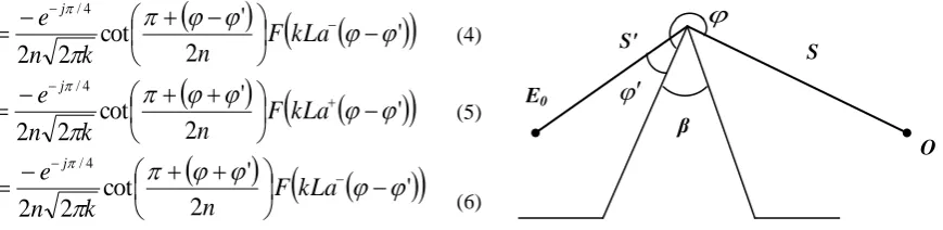
In Fig. 1 a mobile radio wave propagation path in a built-up area consisting of n buildings made of dielectric blocks with rectangular cross-sections is considered. This configuration can be seen as an array of dielectric joint wedges with interior right angles. Each building is
assumed to have the same thickness, spacing, and constant average height relative to the base station antenna. The transmitter can have any arbitrary height (i.e., above, below, or at the same height as the building). As the transmitter is far away from the buildings, so that a plane wave with incident angle α impinges on them.
For the above-mentioned configuration, the diffracted fields were calculated at the observation point (we assumed that the observation point is located at the rooftop of the final building), using the proposed model and considering the effect of the higher order diffracted fields.
Figure 1: Radio wave propagation in presence of buildings.
3. BASICTHEORY
A. Diffraction Coefficient
The field diffracted by an edge is given by [21]:
jksi e i e d
i d
e
s
s
D
Q
E
s
E
)
(
)
(
)
(
(1)
)
(
di
Q
E
is the incident field at the diffraction point Qdand
D
is the diffraction matrix, s is the distance between the observation and the diffraction points and finally theterm
ei is the radius of curvature of the incident wave inthe plane of incidence. When the incident wave front is spherical, it coincides with the distance between the diffraction point and the transmitter antenna (
s
). In order to evaluate the diffraction coefficient for a finitely conducting wedge, we use Lubber’s heuristic coefficient:
0
1 2 ,
3 4
,
,
'
,
L
,
n
,
D
D
D
D
D
sh
sh
(2)
'
2
'
cot
2
2
4 /
1
kLa
F
n
k
n
e
D
j
(3)
E0 E(1) En-1 E(n)
Observation Point
v w
'
2
'
cot
2
2
4 /2
kLa
F
n
k
n
e
D
j (4)
'
2
'
cot
2
2
4 /3
kLa
F
n
k
n
e
D
j (5)
'
2
'
cot
2
2
4 /4
kLa
F
n
k
n
e
D
j (6)F[x] is the Fresnel transition function, which is defined as [22]:
x jxd
j
e
x
j
x
F
(
)
2
exp
2
(7)The angles
and
are shown in Fig.2; k is the wavenumber and n is given by:
2
n
(8)
is the interior wedge angle.In the above formulas, L is the distance parameter given by:
s
s
s
s
L
i i ie i i i e
2 1 2 1
(9)i
2 , 1
are radius of curvature of the incident wave front at the diffraction point. For a spherical incident wave fronts
i i i
e
1
2
and the distance parameter can beshown as follow:
s
s
s
s
L
(10)The function
a
is given by:
2
2
cos
2
2
n
N
a
(11)'
and
N
are the integers which most nearly satisfy the equations:
N
n
2
(12)
N
n
2
(13)Note that
s,h is the Fresnel reflection coefficients ofthe wedge at the edge.
Figure 2: Diffraction by a straight wedge.
B. Model’s Equations
According to the Heuristic solution [23], the field of the 6 times diffracted ray in Fig. 3 can be written as:
o o o o n o n n n m n m m m l l m l i l i N o n m l i o n m l i i i i s s jk o UTD D ks j o D ks j n D ks j m D ks j l D ks j i D s s s s s s e E E T 6 6 6 5 5 5 5 4 4 4 4 3 3 3 3 / 2 2 2 0 , ,
, 1 2
1 7 6 5 4 3 2 ! 1 ! 1 ! 1 ! 1 ! 1 1 0 1
(14)E0 is the incident field at the diffraction
point,
s
T
s
1
s
7, and k is the wave number. Here, D1 to D6 are diffraction coefficients. In this formulathe upper limit N0 stands for a chosen order.
The field in (14) can be rewritten in a simpler form by defining di (m;n) as [23]:
ni m i i n m m i i D ks j m n m d ! 1 , (15)
Using (2), the following compact expression is obtained:
,
,
,
,
0
,
,
0
1
6 5 4 3 2 1 0 7 6 5 4 3 2 0 1o
d
o
n
d
n
m
d
m
l
d
l
i
d
i
d
s
s
s
s
s
s
e
E
E
N o n m l i o n m l i s s jk o UTD T
(16) The expression in (1) can be generalized to more than six wedges. Using the above example, it should be obvious how to generalize the result to more than six edges2.For calculating the diffracted field in the transition zone, we explored and improved the approach presented in an earlier study [17]. The total field at the observation point (Fig. 1) was calculated using the summation of fields produced by a single and multiple diffraction process. In the proposed model, all beams except En-1 are multiple
diffraction terms, En-1 is single diffraction from the last
edge and, therefore, it is not combined with the multiple
2
One explanation for long computation times when the number of edges turns out to be large is that the series in (16) will engage an enormous number of complex multiplications. The computation plan in [23] will reduce the number of complex multiplications significantly.
diffractions. To present an expression for the overall field calculation, the following argument can be used. If there was only one building between the transmitter and receiver, then the received field at the observation point can be given by
jkvx jkv
e
D
v
e
E
E
(
1
)
0 cos1
(17)
The above formula is made out of two terms, the first term accounts the contribution of the direct field, for
0
(17) must be used without this term, and the second term is to calculate the diffracted field. Dx isdenoted as:
D
L
v
D
x,
2
,
2
3
(18)
L
D
,
,
is the diffraction coefficient for an imperfect conducting wedge given in [24]. Furthermore, if the number of buildings is more than one (i.e., when there are a row of buildingsn
2
), then the total received field (E(n)) can be summarized as follows:
1 1 , , cos cos 1 , , 2 0 1 cos 2 1 ) ( 1 2 1 1 2 1 ) ( n p w v p n jk p n b p n p n w v p n jk jkv x jkv n w w v m n jk m n a nm nm n m
m n w w v m n jk m e D vw e p E e D v e E e D w v e E n n E (19)
Da,n,m and Db,n,p are the higher order diffraction
coefficients (their values depend on the number of buildings). The factor of 1/2 in (19) is used to handle the special case of grazing incidence [24]. With reference to Fig.4, if we assume that only E0 and E(1) are the incident
waves at the first and the second wedges, respectively, then the coefficients Da,7,0 and Da,7,1 are given by the
following expressions:
, , , , ,0, , , , , , , , 0 13 12 11 10 9 8 7 6 5 4 0 3 2 1 0 , 7 , 0 v d v u d u t d t s d s r d r q d q p d p o d o n d n m d m l d l i d i d D N A
a
(20)
, , , ,00 , , , , , , , , 0 12 11 10 9 8 7 6 5 4 0 3 2 1 1 , 7 , 0 u d u t d t s d s r d q d q p d p o d o n d n m d m l d l i d i d D N B b
(21)v
u
t
s
r
q
p
o
n
m
l
i
A
(22)
u
t
s
r
q
p
o
n
m
l
i
B
(23) The upper limit N0 is chosen properly (in this paper, N0 = 4). Em is the field impinges on the first corner of the
roofs (left-placed wedge forming the rectangular building cross-section) as indicated in Fig.1. Hence, for
m
1
, Emcan be defined as given in (24). In this formula E(m) is the diffracted field from the last building’s edge and can be considered as a single diffraction field. Thus, Em can be
described as
jkw z jkw w w v r m jk r m d r m r m r m w w v r m jk m r w v q m jk q m c q m q m w v q m jk m m q m e D w e m E e D w v e r E e D vw e E m E 1 ) ( 2 1 ) ( 2 1 2 1 cos , , 1 cos 1 1 , , cos 1 0 (24) zD
is defined as:
D
L
w
D
z,
,
2
3
(25)If the incident fields are E0 and E(1), then Dc,6,0 and Dd,6,1 for seven buildings are given by:
, , , , ,0, , , , , , , 0 12 11 10 9 8 7 6 5 4 0 3 2 1 0 , 6 , 0 u d u t d t s d s r d r q d q p d p o d o n d n m d m l d l i d i d D N B c
(26)
,
,
,
,
0
Figure 3: Ray geometry for diffraction by six straight wedges.
Figure 4: Diffraction mechanism by seven buildings when E0 and E(1) are considered.
4. SIMULATION
The normalized total electric field intensity at the observation point against number of existing buildings by using (19) is shown in Fig. 5, for v =28, w =22, f = 922 MHz, r =5.5, σ=0.023 S/m and hard polarization. Applied
permittivity and conductivity for the diffracting and reflecting building surfaces in the simulation are very close to buildings actual electrical properties.
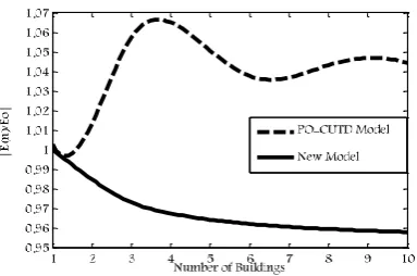
In Fig. 6 the settled normalized diffracted field (for 10 buildings) is plotted against the angle of incidence of the fields α by using both the new model and the PO-CUTD model in [17]. Here v =28, w =22, r =5.5, σ=0.023 S/m,f=922 MHz, it is expected that │E(n)/E0│ is settled in
a fixed value of less than 1, however it is more than one at
α > 5º for the PO-CUTD model and it can be understood there is a critical angle between 5º and 6° in this model. Consequently we can observe from Fig. 6, more rational and explainable prediction is available by using this proposed model.
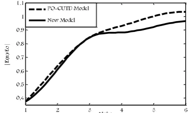
In order to review a special case, the normalized total electric field intensity at the observation point against number of existing buildings by using both the new model and the PO-CUTD model is shown in Fig. 7, for v =28, w =50, f = 922 MHz, r =5.5, σ=0.023 S/m, α = 4° and
hard polarization. Comparison of the two models shows that the PO-CUTD model predicts the amplification while the new model shows the attention. As we know when waves are sent through buildings, it is impossible to be amplified.
Comparing the two different sorts of the results shows
that the new improved UTD-based model provides a prediction that is more acceptable and its trend is more accurate.
Figure 5: The normalized total electric field intensity at the observation point against number of existing buildings.
Figure 6: The normalized total electric field intensity at the observation point against the angle of incidence of the fields, for the new model and the PO-CUTD model.
Source
6
s
5s
4s
3s
1
s
2
s
5
5
4
4
3
3
2
2
1
1
E0
Observation Point
s2 s9 s10 s11 s12 s13
Observation point
s3 s5 s6 s7 s8
s1
s4
E (1) s10 s11 s12 s13 s14
Observation point
s2 s3 s4 s5 s6 s7 s8 s9
s1
Figure 7: The normalized total electric field intensity at the observation point against number of existing buildings, for the new model and the PO-CUTD model.
5. CONCLUSION
In this paper, an improved model expressed in terms of higher order diffraction coefficients for prediction of the multiple diffraction produced by an array of flat roofed buildings considering the plane-wave incidence has been presented. The results showed that the proposed model can correct errors of the PO-CUTD model in [17]. Our results are the perfect examples for approving this subject. However, it is necessary that higher order diffraction coefficients are applied to improve results especially for
α > 4°.
6. REFERENCES
[1] H. L. Bertoni,‖ Radio Propagation for Modern Wireless Systems‖ Prentice-Hall, Englewood Cliffs, NJ, 2000.
[2] COST 231, European Commission, ―Digital mobile radio toward future generation systems‖ Brussels, Belgium, 1999.
[3] W. Zhang, ―Fast two-dimensional diffraction modeling for site-specific propagation prediction in urban microcellular environments,‖ IEEE Transaction o Antennas and Propagation, Vol. 49, No. 2, 428–436, Mar. 2000.
[4] J. Wolfish, and H. L. Bertoni, ―A theoretical model of UHF propagation in urban environments,‖ IEEE Transaction on Antennas and Propagation, Vol. 36, No.12, 1788–1796, Dec. 1988.
[5] S. R. Saunders, and F. R. Bonar, ―Explicit multiple building diffraction attenuation function for mobile radio wave propagation,‖ Electron. Letter, Vol. 27, No. 14, 1276–1277, Jul. 1991.
[6] S. R. Saunders, and F. R. Bonar, ―Prediction of mobile radio wave propagation over buildings of irregular heights and spacings,‖ IEEE Transaction on Antennas and Propagation, Vol. 42, No. 2, 137–144, Feb. 1994.
[7] M. J. Neve, and G. B. Rowe, ―Contributions toward the development of a UTD-based model for cellular radio propagation prediction,‖ Proc. IEE Microwave. Antennas Propagation, Vol. 141, No. 5, 407–414, Oct. 1994.
[8] W. Zhang, ―A more rigorous UTD-based expression for multiple diffractions by buildings,‖ Proc. IEE—Microwave. Antennas Propagation, vol. 142, no. 6, pp. 481–484, Dec. 1995.
[9] W. Zhang, ―A wide-band propagation model based on UTD for cellular mobile radio communications―, IEEE Transactions on Antennas and Propagation, vol. 45, no. 11, pp. 1669–1678, Nov. 1997.
[10] L. Juan-Llácer and N. Cardona, ―UTD solution for the multiple building diffraction attenuation unction for mobile radio wave propagation," Electron. Letters, vol. 33, no. 1, pp. 92–93, Jan. 1997.
[11] A. Kara and E. Yazgan, ―UTD-based propagation model for the path loss characteristics of cellular mobile communications system,‖ in Proc. IEEE Int.Symp. Antennas and Propagation Society, vol. 1, Orlando, FL, pp. 392–395, 1999.
[12] C. Tzaras and S. R. Saunders, ―An improved heuristic UTD solution for multiple-edge transition zone diffraction,‖ IEEE Transactions on Antennas and Propagation., vol. 49, pp. 1678– 1682, Dec. 2001.
[13] L. Juan-Llácer and J. L. Rodríguez, ―A UTD-PO solution for diffraction of plane waves by an array of perfectly conducting wedges,‖ IEEE Transactions on Antennas and Propagation, vol. 50, no. 9, pp. 1–5, Sep.2002.
[14] R. Arablouei and A. Ghorbani, ―A new UTD-based model for multiple diffractions by buildings,‖ in Proc. 3rd Int. Conf. Microwave and Milimeter Wave Technology, St. Petersburg, Russia, pp.484–488, Jun. 2002.
[15] D. Erricolo, G. D’Elia, and P. L. E. Uslenghi, ―Measurements on scaled models of urban environments and comparisons with ray-tracing propagation simulation,‖ IEEE Transactions on Antennas and Propagation, vol. 50, no. 5, pp.727–729, May 2002.
[16] D. Erricolo, ―Experimental validation of second-order diffraction coefficients for computation of path-loss past buildings,‖ IEEE Transaction Electromagnet. Compact, vol. 44, no. 1, pp. 272–273, Feb. 2002.
[17] J.-V. Rodríguez, J.-M. Molina-García-Pardo and L. Juan.Llácer, ―An improved solution expressed in terms of UTD coefficients for the multiple-building diffraction of plane waves,‖ IEEE Antennas and Wireless Propagation Letters, vol. 4, 2005.
[18] E. Torabi, , A. Ghorbani and H.R. Amindavar, ―Modification of the UTD Model for Cellular Mobile Communication in an Urban Environment,‖ Electromagnetics, Vol. 27, 263-285,Jun. 2007. [19] A. Tajvidy, and A. Ghorbani, ―A New Uniform
Theory-of-Diffraction-Based Model for the Multiple Building Diffraction of Spherical Waves in Microcell Environments,‖ Electromagnetics, Vol. 28, 375-388, Jun. 2008.
[20] E. Torabi, A. Ghorbani and A. Tajvidy, "A Modified Diffraction Coefficient for Imperfect Conducting Wedges and Buildings with Finite Dimensions" IEEE Transactions on Antennas And Propagation. Vol. 57, No. 4, 1197-1207, Apr. 2009.
[21] R. G. Kouyoumjian and P. H. Pathak, "A uniform geometrical theory of diffraction for an edge in a perfectly conducting surface". Proc. IEEE. Vol. 62, 1448–1461, 1974.
[22] M. F. Catedra and Jesus Perez-Arriaga, Cell Planning For Wireless Communication, Artech House, Inc., 1999, ch. 9.
[23] P. D. Holm, "Calculation of Higher Order Diffracted Fields for Multiple-Edge Transition Zone Diffraction", IEEE Transactions on Antennas and Propagation, Vol. 52, No. 5, pp. 1350-1355, MAY. 2004.