TEC H N I C A L R E P O R T

(1)

I N S P E C T A

T E C H N I C A L R E P O R T

Master’s Thesis

Determination of Safety Factors in High-Cycle

Fatigue

-

Limitations and Possibilities

Robert Peterson

Supervisors:

Magnus Dahlberg

Christian Walck

Report No.: Revision No.: INSPECTA TECHNOLOGY AB

(2)

Report No.: Revision No.:

Date

9/18/2012

Our project No.

Approved by Organizational unit Inspecta Technology Customer Customer reference Summary

This thesis evaluates different methods for determining safety factors in the risk analysis of a system subject to high-cycle fatigue. This is done by solving a model problem and comparing the results. Apart from comparing the precision and effectivity of the methods, the analysis attempts to determine some limitations that the

methods might face in application. Comparing the results calculated with the help of a Monte Carlo simulation

to the Sensitivity Analysis, the discrepancy between the methods appears to be negligible, as long the

uncertainties in the model are kept low. Increasing the errors may result in high discrepancy between the methods. The choice of distribution to model the variance in the input parameters appears to only be negligible

down to a prescribed probability of failure . If the governing distributions of the model are not known,

only the result that is independent of distribution is a reliable measure for reliability.

Report title

Determination of Safety Factors in

High-Cycle Fatigue - Limitations and

Possibilities

Subject Group

Index terms

Work carried out by

Robert Peterson

Distribution

No distribution without permission from the customer or Inspecta Technology AB. Limited internal distribution in Inspecta Technology AB.

Unrestricted distribution. Work verified by

Date of this revision

(3)

1 NOMENCLATURE ... 4

2 MOTIVATION ... 4

3 FORMULATION OF THE PROBLEM... 6

3.1 High-Cycle Fatigue ... 6

3.2 Correction Factors ... 7

3.3 Safety Factor ... 8

4 FIXED LOAD AMPLITUDE ... 9

4.1 Analytical solution for the special case ... 10

4.2 Sensitivity Analysis ... 12

4.3 Monte Carlo ... 12

4.4 Other Distributions ... 15

4.5 Analysis of the Results ... 16

4.6 Summary ... 22

5 UNCERTANTY IN LOAD AMPLUITUDE ... 22

5.1 Method ... 22

5.2 Result ... 23

6 CONCLUSIONS ... 24

7 APPENDIX ... 25

7.1 Generation of Random Numbers ... 25

(4)

1 NOMENCLATURE

Probability function Strength

Load

Cumulative distribution function Probability distribution function Probability of failure

Standard deviation Expectation value Variance

Coefficient of variation

Expectation value of the normal distribution Uniformly distributed random number Strength measured in lab

Corrected strength Size factor

Surface finish factor Notch sensitivity factor Safety factor

Lognormal distribution

Normal distribution

Weibull distribution

2 MOTIVATION

This thesis addresses the problem of predicting the reliability of an engineering system that is governed by variability. The focus is particularly set on the problem of estimating risks of failures which seldom occur, but can have serious consequences. In order to be able to estimate the probability of failure, a physical model of the system is developed as a function of variables that vary with different probability distributions.

Consider, for example, the function that describes the ways the system can fail. The reliability of the system

can then be written explicitly as the probability of failure, in the following notation . A common

situation seen in engineering systems is when can be described as a function h of random variables being less

than some critical value , (Rychlik & Rydén, 2010).

where are random variables with subjectively chosen distributions.

A common way to model is in terms of the system strength and the load that is imposed on it, (Rychlik &

(5)

described by a single random variable each. This allows us to interpret the reliability of such a system in the

form of a resulting random variable .

(1)

The failure of the system, in this case, occurs when the load on the system exceeds its strength. The probability

of failure, , is therefore given by

₍₂₎

There exists numerous ways of estimating this probability as well as numerous ways to design a physical system to carry out its intended performance during a certain lifetime, and only fail with a probability that does not exceed a prescribed value. A few common methods in risk analysis will be considered in this paper, and their properties will be compared.

One of the methods that this thesis will evaluate is the Monte Carlo (MC) simulation. This is a popular tool, since the precision of the result can be chosen arbitrarily by iterating the procedure until the desired precision is reached. Also, assuming that the physical model is correct, the probability distributions of the variables are true and that you are using a fair uniform random number generator, there is no difference between that MC

simulation and a fair experiment in real life. Modern computers also allow you to simulate your experiment until the desired precision is reached for most applications in risk analysis. However, to achieve perfection in any of these above mentioned criteria, for a fair MC simulation, is obviously very hard.

In the work done by Sara Lorén et al. (Bergman, de Maré, Lorén, & Svensson, 2009), the MC simulation is compared to a so called Sensitivity Analysis (SA). In this method, the physical model is (as in the MC

approach) constructed in the form of a function of random variables, where the random variables have a given expectation value and variance. The variance in the model is then determined by the general formula of error propagation for independent random variables.

√( ) ( ) ( ) ( )

(

3

)

By using this equation, the standard deviation is calculated and the quantile from a chosen probability

distribution can be used to determine the . This is definitely a much faster method than the MC simulation.

Also, the partial derivatives under the square root in equation

(3)

gives a measure of which parameter

contributes most to the variation in the model.

Sara Lorén et al. (Bergman, de Maré, Lorén, & Svensson, 2009) describes that when calculating the due to

variation using the MC simulation, the final result depends both on the physical model and the chosen

distribution of the random variables. The SA, on the other hand, does not demand that we know the distribution

of the random variables. It only demands that we know their expectation values, , and variances, . This

is very convenient since it may save a lot of computation time. Nevertheless a choice of the distribution needs to be made in both methods. In the MC case, every random number needs to be selected from a distribution, and in the SA case the determination of the quantiles (as mentioned above) needs a choice of a distribution. As

mentioned before, assuming that the choice of the distribution is correct, the MC simulation gives a correct result given enough simulations. However, both the physical models and assumed distributions are usually only an approximation of the real system, and the error is not always known.

According to the work done by Sara Lorén et al. (Bergman, de Maré, Lorén, & Svensson, 2009), the largest difference between the two methods lies in the evaluation of the high quantiles (corresponding to the outer tails

(6)

of a system is often very undesirable. Therefore the is kept low and the quantitative evaluation demands an

accurate knowledge of the far end tails of the distributions.

Conclusively, MC and SA are two methods that give different results. Can any of these two methods be used in a quantitative analysis of the engineering system that demands high reliability? If the choice of the input distributions is not a negligible factor in the final result, when does the model error become the dominant error source for the final result?

These questions lead towards the main motivation of this thesis. The working hypothesis is that the demand on the reliability of the type of systems that is mentioned above, corresponding to a low probability of failure

_{, is unreasonable, unless the distributions of the random variables are known.}

3 FORMULATION OF THE PROBLEM

The analysis presented in this paper is general in the sense that it can be applied to any mathematical model containing stochastic variables. However, the main focus will be turned towards a specific application, namely fatigue in material in the form of progressive and localized structural damage that occurs when a material is exposed to cyclic loading.

3.1 High-Cycle Fatigue

Since the middle of the 19th century, engineers have known that cyclic loading (repeated loading and

unloading) on a material can cause fracture even though one single applied load of the same magnitude would not. If the cyclic loading is applied with a magnitude above a certain threshold, microscopic cracks will begin to form at the surface of the material. With continued cyclic loading, the crack will grow until it reaches a critical size that will finally cause a sudden fracture. This process is classified as High-Cycle Fatigue (HCF) and refers

to situations when the number of cycles is of the order of magnitude , or more, (Sundström,

1999).

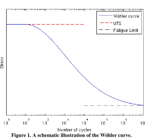
The measurement of load amplitudes that causes fatigue is done in the lab by either pulling, pressing, turning or bending test rods in a repeated manner. In the simplest experiment of this type, the rods are cylindrical with a polished surface, 10 mm in diameter and taken from materials that are 20 mm in diameter. The result of such an experiment is presented in an S-N-diagram, also known as a Wöhler curve. A schematic illustration of a typical

Wöhler curve is shown in

Figure 1

. The curve is constructed from experimental results where each data point is

produced by exposing test rods to cyclic loading of constant amplitude. Each test is continued until the rod fractures, so that the number of cycles to failure can be recorded in the graph. Each amplitude is tested a number of times to obtain an error in the result. The Wöhler curve is then usually constructed to represent a 50% risk of failure. This implies that the Wöhler curve represents the median value for the strength of the material that is exposed to cyclic stress.

(7)

Figure 1. A schematic illustration of the Wöhler curve.

The Wöhler curve roughly consists out of three distinct parts. For high stress amplitudes, the curve can be approximated with a slope that approaches to zero. The straight line that tangent to this slope is called the ultimate tensile stress (UTS), and corresponds to the maximum stress that a material can withstand before permanent deformation occurs. The second part of the curve has a fast negative slope that connects to the third line, which also approaches a slope equal to zero. The third part of the slope is usually approximated by a straight line called the fatigue limit. The test rods that are exposed to cyclic stress of amplitude lower than the

fatigue limit have a 50% of never failing during the experiment. If a test rod doesn't fail after approximately 107

cycles, the experiment is aborted and the rod is assumed to have an infinite lifetime. The fatigue limit is what decides the limitations on the design of engineering systems that are desired to have an infinite lifetime, (Sundström, 1999), (Nilsson, 2001).

3.2 Correction Factors

The resulting fatigue limits that are produced in the lab, in the form of a Wöhler curve, are empirically determined for test rods whose dimensions and properties are very different from structures in a lot of

applications, i.e. buildings, vehicles, bridges etc (see Section 3.1 for dimensions). Therefore, we can expect that the Wöhler curve in real applications assumes different values, even if it conceptually remains unchanged. The paradigm in modern risk analysis of HCF is to use empirical factors that correct the values produced in the lab. The correction factors that are used are found in tables and graphs, in specific literature (Rules for the design of cranes part 2: Specification for classification, stress calculations and design of mechanisms, London, 1980). When modeling the strength of a system in this paper, factors that correct for three different effects will be used. The factors will correct for the difference in size, the surface finish and the notch effect which changes the stress

concentrations locally in real systems. For simplicity, the factors will be given the following notation , and

for, size, surface and notch effects respectively. The strength of a system , will be determined by reducing

the value of the strength measured in the lab (using test rods) , in the following way.

(8)

In real applications, these correction factors are chosen by looking up table values, approximating from graphs, using previous experience in the field and experience of similar problems. Deciding the uncertainty in the evaluation of these correction factors is therefore not an easy task. This paper will however not draw any conclusions based on the magnitude of any input data. Instead, the focus will be turned towards the

understanding of the relationship between input data, input errors, subjective statistical distributions, numerical methods and model assumptions. All of these quantities and concepts will be varied within the natural limits that usually occur in the risk analysis of HCF.

3.3 Safety Factor

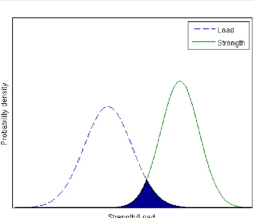
As mentioned in the previous section, a model for reliability can be constructed with the help of two functions of random variables. One describing the system strength and the other one describing the load imposed on the

system, see again equations

(1)

and

(2)

. Assuming that the strength and load vary independently, the two

functions can be described by two independent probability distribution functions (PDFs).

Even when the engineering system is constructed so that the expected value of the strength is greater than the expected value of the load, the statistical variation in both quantities gives a probability of the opposite to be true. Since the behavior of two independent probability distributions needs to be considered, the calculation of

the becomes a problem of two variables. We want to find out the probability of the load to be a certain value

given that the strength assumes a value so that . According to the theory of probability, when

evaluating the conditional probability of two quantities having independent distributions, say and ,

the probability of being less than is given by the following integral, (Rychlik & Rydén, 2010).

∫ ∫ ∫ ∫

(

5

)

As is seen in equation

(

5

)

, this double integral can be rewritten to a single integral using the cumulative

distribution function (CDF) of the strength rather than the PDF. This result will be used later in this thesis. A

(9)

Figure 2. A schematic illustration of the overlap between the PDFs of strength and load. Note

that this figure is a simplification. To obtain the

using the PDFs of the strength and loadn the

calculation must be done in two dimensions.

In order for an engineering system to be robust, a demand must be set on the relationship between the strength

and the load that insures that the is kept under a prescribed value. With the help of a statistical analysis, the

system can be designed so that the safety requirement is met. After doing so, by convention, a so called safety

factor ( ) is calculated. It is defined so that it is high when the calculated is low and vice versa. The is defined as the ratio between the median values of the strength and the load of the system (median of variable

will be denoted ̃).

̃ ̃

(

6

)

A is a more crude measure of reliability than considering the directly, since the same median value for

different distributions can give a different result for the . However, in practice, there are certain cases when

the uncertainties in data are too large or when there isn't sufficient information to compute the risks. In those

cases, the from similar systems encountered in the past can serve as a good measure for reliability, since it is

supported by previous calculations and experience in the field.

4 FIXED LOAD AMPLITUDE

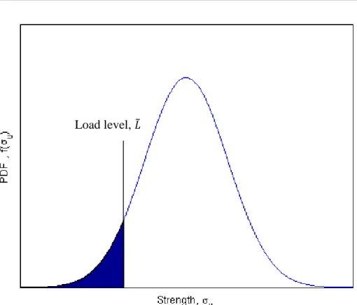
Let us first consider the simple case where the strength of the system is described by equation

(4)

, and a fixed

load amplitude (no uncertainty).

Figure 3

schematically illustrates the probability distribution function of the

strength and the fixed load. The shaded part represents the . In real applications, you would demand the to

be less than approximately . So, in practice, you will want to design your system so that the shaded

(10)

Figure 3. An Illustration of the tail of the distribution that is considered when modeling for fixed

load.

As mentioned earlier, the aim of this thesis is to compare different methods for calculating reliability in risk analysis. In order to be able do that, a model problem is chosen that describes a typical problem in risk analysis

of HCF. The median values and errors chosen for parameters that model strength in equation

(4)

are given in

Table 1

.

As mentioned in section 3.2, deciding a typical variation in a correction factor is not a trivial task. A proposed engineering approximation is obtained by subjectively choosing the maximum and minimum value for a

correction factor and assuming that this interval corresponds to 2 standard deviations, see equation

(

7

)

.

(

7

)

The strength measured in the lab, , was on the other hand given a value of the median and variation that could

typically be obtained from an S-N-diagram.

Parameter Median Value Coefficient of variation

300 [MPa] 0.150

1.2 0.042

1.08 0.012

1.85 0.036

Table 1. Median values and errors of the input data for the model problem with fixed load.

4.1 Analytical solution for the special case

To be able to evaluate the accuracy of the different methods in risk analysis, a comparison will be made to a special case where an analytical solution for the ratio of random numbers is possible to achieve. This is done by

(11)

applying a logarithmic transformation on equation

(4)

and assuming that the variables , , and are

independent and lognormally distributed.

According to the definition, if a random variable

. Since the sum of normally

distributed variables is a normally distributed variable,

. The mean and variance of this sum of

normally distributed variables is given by the relations below. Remember that the mean is equal to the median for the normal distribution.

Now, since we know that moments of the distribution of strength are easily calculated, we would like to

determine the that corresponds to a prescribed , and determines the relationship between the strength and

the load. Assuming that the strength and load are lognormally distributed and applying a logarithmic transform

on equation

(

6

)

results in the following equation

̃ ̃

̃

Now introducing new variables ̃

,

and

, we can set up the following equation

Since failure occurs with probability , the following equation can be set up

̃ ̃ √

√ √

Now for fixed load, the standard deviation of the load can be omitted. Since the logarithmic transform has been

applied on , the following approximation can also be used with great success, (Bergman, de Maré, Lorén, &

Svensson, 2009).

̃

The for the system of fixed load can finally be expressed simply as a function of the coefficients of variation

(12)

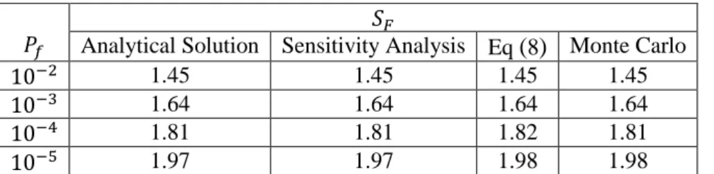
Choosing to be a quantile for a certain probability of failure, expressed in terms of standard deviations, gives

the corresponding . The result of solving the model problem using equation

(

8

)

is given in

Table 4

.

Looking again at equation

(

6

)

, note that since the load is fixed, it can be very conveniently replaced by an

arbitrary quantile, , of the distribution of strength. This quantile will then correspond to the of the system,

see again

Figure 3

for illustration.

̃ ̃

̃

₍

₉

₎

The quantiles of the distribution of strength, corresponding to both the median and an arbitrary , are easily

determined by numerically calculating them with the help of the CDF, see

Figure 4

. Since the CDF of the

lognormal distribution does not have an algebraic form, in the general case, it is calculated numerically. The

result is shown in

Table 3

.

A numerical experiment was performed to show that the error in the numerical approximation of the CDF,

produced by the built-in function in MATLAB, is negligible, see

Table 2

.

Step-size [MPa] 1 1.4497 1.6379 1.8105 1.9761 0.1 1.4494 1.6372 1.8100 1.9747 0.01 1.4494 1.6372 1.8100 1.9747 0.001 1.4494 1.6372 1.8100 1.9747

Table 2. Numerical experiment for determination of accuracy.

4.2 Sensitivity Analysis

As mentioned in section 2, the SA simply uses the general formula of error propagation to calculate the standard deviation in the distribution of strength. Particularly for the model problem, this means that

√( ) ( ) ( ) ( )

(

10

)

The variation for every quantity in equation

(

10

)

is calculated using the median values in

Table 1

and assuming

that all parameters vary lognormally. The partial derivatives are calculated analytically, to eliminate this error

source. The expectation value of is simply assumed to be given by equation

(4)

. Once again, calculating the

moments of the distribution of strength allows the CDF to be produced numerically and the safety factors to be

calculated using equation

(

9

)

. The result is given in

Table 3

.

4.3 Monte Carlo

Consider again this model problem given by equation

(4)

. In the general case the random variables modeling

strength are not necessarily lognormally distributed. This creates a new problem, since in the general case, the

product ( ) is no longer distributed the same way as the factors on the other side of equation

(4)

. In fact the

distribution of the product is not necessarily distributed by any standard distribution at all. This means that

determining the moments, and therefore also quantiles and , for such a distribution becomes non-trivial. There

are often ways of expressing the distribution of a product of random variables analytically, but the answer doesn't necessarily come out in an algebraic form (as for the normal distribution), and numerical integration or

(13)

other approximations are needed for evaluation of the . In a simple case, where there is only one equation

describing the reliability of the system, as in this model problem, there is eventually one integral that needs to be solved to get the distribution of the product. A real system can however, very fast, become much more complicated. Different modes of failure can branch out into trees where every branch may be described by a non-trivial distribution for reliability.

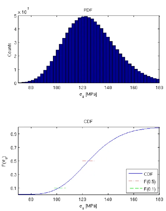
This is when a MC simulation can come in handy. Given only the distributions of the input parameters, the MC simulation can empirically construct the output distribution regardless the model and input distributions. The MC simulation is, as mentioned, an empirical method, hence the result contains an error. However, the longer you run the simulation, the higher is the precision of the result, see Appendix the description of the generation of random numbers.

In order to be able to evaluate the error of this method, the same input data as in the analytical case was used, see

Table 1

. The simulation was then run by generating one random number from the lognormal distribution of

each parameter in equation

(4)

, and in this way calculating the strength, . The strength was then calculated in

this way many times, until the distribution of could be evaluated with the prescribed precision. The result is

illustrated in

Figure 4

. The empirical PDF of is seen in the top plot, and the empirical CDF is seen in the

bottom plot. The was calculated numerically reading off the median the relevant quantiles in the empirical

CDF. The resulting for different values of are presented in

Table 3

. The result using the MC simulation

was calculated using simulated values of .

Analytical Solution Sensitivity Analysis Eq

(

8

)

Monte Carlo

_1.45 _1.45 _1.45 _1.45

_1.64 _1.64 _1.64 _1.64

_1.81 _1.81 _1.82 _1.81

_1.97 _1.97 _1.98 _1.98

Table 3.

calculated with three different methods, for lognormally distributed input data.

In comparison to the analytical solution, the result of the MC simulation shows good accuracy, with the value of

the differing only in the third digit for the . This discrepancy comes from the fact that this

corresponds the far end tail of the distribution where the statistics are only made based on the values of that

occur only once every 100,000 simulations. With simulated values, it is expected that approximately 1000

of them were used for evaluation of the corresponding to the .

simulations can take a lot of computation time, and a vector will take up more computer memory than

most platforms have available. However, in practice, there are only two values that need to be stored, the

median and the quantile corresponding to the desired . Looking at the bottom plot in

Figure 4

, it is easy to

see that it is enough to save only a few simulated values of around the median, and the tail of the CDF only

up to the value of the needed quantile. With a qualified guess of the quantiles, after a look at the result from a shorter simulation, it is possible to cut down the simulation time to a few hours and a reasonable requirement on the available computer memory. It is worth to remember that the median value has very little dependence on the outliers of the distributions. The plots representing the PDFs and CDFs in this thesis are made with a number of

simulations that is sufficient for proper visualization. The complete distributions with trials were never

(14)

Figure 4. The top figure shows a PDF calculated using the MC simulation for the lognormally

distributed data. The bottom figure contains the corresponding CFD calculated with the help of

the same simulation. The 0.5 (median) and 0.1 quantile are highlighted.

Now, after solving the model problem with the help of two different methods (MC and SA), it can been seen that the result is quite accurate for both of them, compared to the analytical solution. This is however not too surprising. As mentioned in Section 2 there is no reason why there should be a significant error in the MC simulation, it is only a matter of running enough simulations before you reach the an accurate result. Also, the

approximation given by equation

(

8

)

seems to give an error of up to only about 1%, which is also a satisfying

result in this application.

An error in the SA might be expected since it does not take into account that product of random variables is not distributed as the distribution of the factors, in general. However, the lognormal distribution happens to be a

(15)

special case in this regard. It can be shown that both product and ratio of lognomally distributed random numbers is lognormally distributed. That is why it becomes interesting to find out how much the result can differ if other distributions are involved in the risk analysis, and what kind of effect the variation of the input parameters can have on the result. This issue is addressed in the next section.

4.4 Other Distributions

The Weibull distribution is often used to model strength of a system in risk analysis, therefore it is a suitable choice for this analysis. Since the normal distribution is a popular choice for modeling any stochastic variable, it is also interesting what difference it can make in the result. However, it is worth remembering that the normal distribution assumes that the variation for the model parameters is symmetrical in both positive and negative direction of the x-axis. Since negative values of the strength or the correction factors does not make sense, the normal distribution has very clear disadvantages. The Weibull is, on the other hand, equal to zero for negative numbers, and the lognormal distribution is not defined for negative numbers.

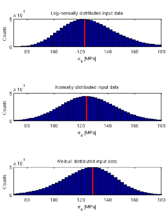
The Monte Carlo simulation was run again using the same input median values and coefficients of variation,

simulating values for the strength . This time all four parameters in equation

(4)

were first randomly

chosen from normal distribution and then chosen from the Weibull distribution. The safety factors were again calculated by setting up the CDF and numerically reading off the median and the relevant quantiles for each

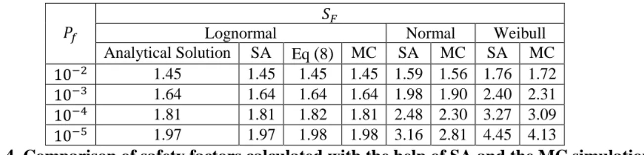
simulation. The result of this calculation is summarized in

Table 4

, where it is also compared to the result

calculated with the help of the SA for the same choice of distribution.

The choice of method (SA or MC) did not appear to be very significant. The differences in the calculated safety

factor is less than 0.05 for and about 0.1, 0.2 and 0.4 for equal to , and

respectively. On the other hand, the choice of distribution shows a difference of up to 2 safety factors for

_.

Lognormal Normal Weibull

Analytical Solution SA Eq

(

8

)

MC SA MC SA MC

_1.45 _1.45 _1.45 _{1.45 1.59 1.56 1.76 1.72}

_1.64 _1.64 _1.64 _{1.64 1.98 1.90 2.40 2.31}

_1.81 _1.81 _1.82 _{1.81 2.48 2.30 3.27 3.09}

_1.97 _1.97 _1.98 _{1.98 3.16 2.81 4.45 4.13}

Table 4. Comparison of safety factors calculated with the help of SA and the MC simulation

using three different distributions.

Looking closer at the three different distributions produced by the MC simulation, it is seen that they differ

mostly in their skewness relative to each other.

Figure 5

illustrates this fact by highlighting the mode

(maximum value of the PDF) for every distribution. The product of lognormally distributed factors produces a distribution skewed to the left, the Weibull case is skewed to the right and the normal case is in between. This fact has a strong impact on the form of the far end tails of the distribution. Skewness to the left (log-normal case) results in a short left-hand-side tail of the distribution. This means that the value of the quantile

corresponding to the , for instance, is closer to the median then in the other distributions. This results

in a lower value of the , see equation

(

6

)

. The opposite is true for the Weibull case, where the skewness to the

(16)

Figure 5. MC simulation of the distribution of the strength assuming that the variation in the

input parameters is strictly lognormal, normal and Weibull distributed respectively. The mode

of each distribution is highlighted.

4.5 Analysis of the Results

If skewness now has a key impact, it is interesting to see what happens when higher uncertainties are used as input data in the model, since high errors in ratios of random numbers tend to produce left-skewed distributions.

Remember that a function is a fast growing function towards infinity as , for any constant ,

while the decreasing behavior after reaching is far less dramatic. This means that the ratio will deviate

(17)

As mentioned in section 3.2, determining the uncertainties in the correction factors is not a trivial task. This fact

gives us a reason to try to see what happens when the input errors are greater than the ones given in

Table 1

,

without creating a far too unreasonable model for the reliability of the system.

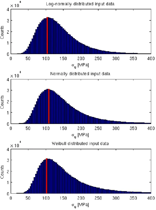
Figure 6

shows the three distributions produced by the MC simulation after increasing the coefficient of variation for each correction factor to 0.20 . The first thing to notice in this figure is that all three distributions are skewed to the left. Second of all, the left-hand-side tails of the distributions are much more similar to each

other. This effect is also seen on the quantitative level in

Table 5

. The differences between the models appear to

have partly dissolved. The analytical solution for the lognormal distribution is also given in the table for the evaluation of accuracy.

Figure 6.

The MC simulation of the distribution of the strength assuming that the variation in the input parameters is strictly lognormal, normal and Weibull distributed respectively. The coefficient of variation is increased to 0.20 for each correction factor. The mode of each distribution is highlighted.

(18)

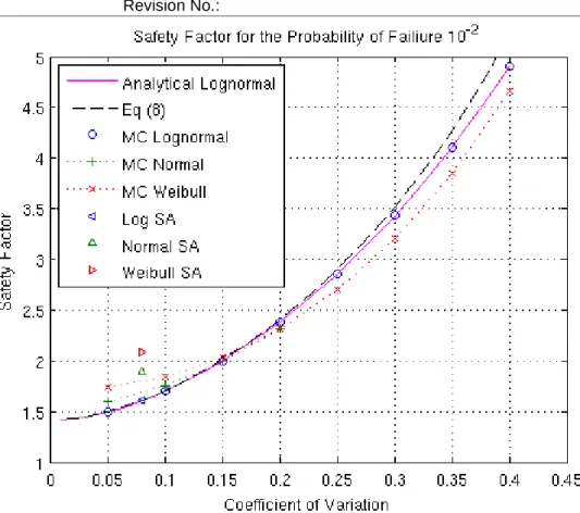
Lognormal Normal Weibull

Analytical Solution SA Eq

(

8

)

MC SA MC SA MC

_2.39 _2.37 _2.39 _2.24 _2.31 _{4.26 2.31}

_3.18 _3.15 _3.18 _2.92 _3.01 _{9.36 3.13}

_4.02 _3.98 _4.02 _3.63 _{3.77 20.67 4.20}

_4.93 _4.87 _4.95 _4.38 _{4.65 45.48 5.59}

Table 5. Safety factors calculated after increasing the coefficients of variation for the correction

factors to 0.20.

With this result, it is interesting to see what the continuous behavior of this transition looks like. Let's first just

look at the analytical case in

Figure 7

. As the distribution skews more and more to the left, the mode starts to

appear to the left of the median. At the same time as the left-hand-side tail becomes shorter. This is the reason

why the value of the accelerates fast to higher values as the coefficient of variation increases.

Figure 7. The effect of increasing the input errors modeling the strength of the system.

By choosing to look at one at a time, it is possible to see this variation for all three distributions in

Figure 8

-Figure 11

. The safety factors are calculated with the help of the MC simulation for all three distributions and also analytically for the lognormal distribution.

(19)

Figure 8.

corresponding to a calculated for varying the coefficients of variation for the correction factors.

Figure 9.

(20)

Figure 10.

Figure 11.

(21)

All three graphs basically have the same kind of behavior. The curves start out at different values, at some point they cross each other and then they continue by diverging away from each other. This behavior explains why

the safety factors calculated with different models in

Table 4

and

Table 5

started by showing very different

values and then came closer to each other. It is also worth remembering that when running the MC simulation for normally distributed input data, high enough errors and number of trials lets the correction factors assume negative numbers. This leads to unreasonable results, thus the lack of exhaustive data in the figures for the normal case.

Finding the solution to the same problem using the SA is a far more trickier task. Instead of producing this skewed distribution, the SA calculates the expected value and variation of the strength and the assumes that it is distributed by some known distribution. Since the distribution of the product is very different from the

distribution of the factors (when errors are high), the assigned distribution is very different from the actual distribution.

Before looking at results of the SA, it is important to mention that assuming a normal distribution creates problems when the coefficients of variation are high. The expected value of the distribution of strength is approximately the same for both methods. Therefore assuming that the strength is distributed symmetrically, and not skewed, results in a much longer left-hand-side tail. This leaves the quantiles corresponding to a

_{on the negative side of the x-axis already for coefficients of variation equal to ≈ 0.1, see}

_{Figure 12}

_.

Figure 12.

The three distributions that are evaluated when calculating the safety factors using the SA for the problem with increased errors.

Also, it is important to remember that even though the Weibull distribution is defined as equal to zero for negative values, it does not fall to zero as fast as the lognormal distribution when the errors are high. This effect

is illustrated in

Figure 12

, which explains the surprisingly high values for the calculated in

Table 5

.

The solution for the coefficients of variation equal to 0.08 using the SA is highlighted in

Figure 8

-

Figure 11

.

The deviation between the methods for with these large errors is almost as high as for the

(22)

good approximation when the errors are high. When the errors are, on the other hand low, the distribution of the product will be very different from the factors making this approximation valid.

4.6 Summary

Turning to the main issue of this thesis, it is interesting to evaluate the methods used in this section and decide to what extent they can be used in the determination of reliability of a physical system governed by the effects of variation.

The model problem with a fixed load was solved with the result given in

Table 4

. The solution showed little

dependence on the choice of method. Also, the safety factors calculated with both SA and MC varied very little

for all three distributions for the prescribed . If higher reliability is not necessary, calculating safety

factors can be done very easily with the help of equation

(

8

)

. For lower , the safety factors differed up to 0.4.

The error of this order of magnitude is not very significant considering that there is no estimation of the model error. The choice of distribution to model the random variables, on the other hand showed to be far more

significant already for . In the case when the distribution is known, the difference between the

methods is so little that the computation time needed for a MC simulation is not motivated compared to the SA. On the other hand the Wöhler curve is usually determined with the help of approximately 25 tests. This does not give enough statistics for the determination of the distribution.

Increasing the errors resulted in skewed distributions. This fact had a big impact on the difference between the safety factors calculated with the two different methods as well as on the difference between the assumed distributions. The ratio of random numbers with high errors seems to be a case that needs to be handled with care.

In any case, even though the SA is an approximate method while the MC simulation calculates a correct result given enough simulations, the MC simulation is not the obvious choice of method. It is important to remember that if there is a high dependence on the choice of distribution in the method, the result calculated by the MC simulation is only useful if there is a reason to believe that the choice of distribution is correct. If the

distribution of the varying parameters is not known, only the solution that is independent of distribution is a reliable one.

5 UNCERTANTY IN LOAD AMPLUITUDE

Now after running various tests on the model of fixed load, it is interesting to see if the results achieved in the previous section hold for a model with a varying load. The varying load does not introduce any new concepts,

other than those illustrated in

Figure 2

. However, the calculation of the brings on a few complications that

need to be considered carefully.

The load will be modeled simply by assuming that it is distributed by a lognormal distribution. This is a convenient model for this analysis since it can be solved analytically and does not assume negative values, as previously mentioned. The variation of the load is given a coefficient of 0.10, while the median value is varied

in terms of the , to see how this affects the . The main idea here is to model the variation of both strength

and load, as schematically illustrated in

Figure 2

, and then alter the to see how it affects the .

5.1 Method

Now since the calculation of the will involve the interference of two independent PDFs, a combination of

their properties will have to be taken into account. There are several ways of calculating such, so called,

conditional probabilities. The most straight forward method, from a pedagogical standpoint, is by using the MC simulation to generate one value of the strength and one value of the load at a time, from their respective distributions, and calculating their difference.

(23)

The is then simply given by the amount of times the difference per total number of trails. The

drawback of this method is that you, as in the previous section need a lot of computation time to achieve a

quantitatively reliable value of the . There is however no need for storing a lot of data, since there are only

two numbers needed to be stored. The number of times and the total number of trials.

An easy way of using the SA is to first calculate the moments for the distribution of strength and load and then

use them in the evaluation of the integral in equation

(

5

)

. The analysis in this thesis used the built in functions

of MATLAB to numerically estimate the PDFs, CDFs and to calculate the integral. The calculation was run with shorter and shorter integration steps until the result converged to a value of needed precision.

5.2 Result

The model with a varying load was analyzed using the input data from

Table 1

for the strength of the system.

Three different MC simulations were again used in the analysis to model the variation in the parameters of strength by the lognormal, normal and Weibull distribution. The SA was used analogously for three different

distributions of strength in equation

(

5

)

. The result is presented in

Figure 13

.

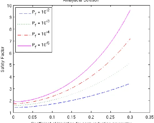
Figure 13.

The for the model with varying load. The input data for strength is given by

Table 1

and the load is modeled by a lognormal distribution with a coefficient of variation equal to 0.10 and the

median determined by varying the .

The same conclusions that were drawn for the results using a fixed load seem to hold for varying load. The difference between using MC or SA is not significant, but choice of statistical distribution shows a deviation of the result of approximately the same magnitude. The choice of distribution seems to be a dominating factor, for this model, as it was for case of fixed load. When the distribution of strength is skewed to the right, as in the Weibull case, the long left-hand-side tail creates a greater overlapping area between the distribution of strength

(24)

where the distribution of strength is skewed to the left creating a short left-hand-side tail, the is lower, see

again

Figure 5

for comparison.

Increasing the coefficients of variation for the correction factors to 0.10 does not change any conclusions either, see

Figure 14

. Both method and distribution has a significant impact on the result for . The overlap between the distribution of load and strength is very different depending on the skewness originating from the ratio of random numbers. This effect is taken into account by the MC simulation, but not for the SA.

Figure 14. Increased coefficients of variation for the correction factors to 0.10, compared to

Figure 13.

The approximation used in equation

(

8

)

shows again to be very good, for the lognormal case. It is so close to the

analytical case, that it is really not possible to read off the difference between them, in these graphs. This is true for both the model problem and for the increased coefficients of variation to 0.10.

6 CONCLUSIONS

Given a distribution that models the uncertainty in the parameters of the model problem, the result shows a negligible dependence on the calculation method, see Figure 13. Therefore the discrepancy between the results calculated by SA and MC can be considered negligible in this application. Since there is no estimation of the error in the physical model, there is no reason to demand a higher precision in the result. If the model

parameters are assumed to be modeled by the lognormal distribution, the safety factors can be calculated with the help of simple expression given by equation (8).

When the properties of a system subject to high-cycle fatigue are determined experimentally in an S-N-diagram, the statistics are usually too low to be able to evaluate the governing distributions. Unfortunately, the choice of distribution can have a highly non-negligible effect on the result, especially when the far end tails of the distributions are evaluated. Figure 13, specifically, shows that the safety factors calculated for a prescribed

(25)

Apart from the choice of distribution, the far end tails are also affected by the magnitude of the variance in the model parameters. High variance results in a skewed distribution of the system. This effect is taken into account by the MC simulation, but not by the SA. Therefore a non-negligible discrepancy between the methods is seen

already for a low , see Figure 14.

A reliable estimation of the far end tails of a distribution demands that a lot of trials are made, and this may increase the computation time significantly. However, checking the skewness can be done with a relatively few simulations. By doing so, a decision of whether SA is a good approximation, can be made.

Nevertheless, it is important to remember that if there is a high dependence on the choice of distribution in the model, the result calculated by the MC simulation is only useful if there is a reason to believe that the choice of distribution is correct. Otherwise only the result that is independent of this choice is a reliable measure of reliability. If the input errors are low enough, however, the SA will give a good estimation and may save a lot of computation time.

In short

 The result is independent of the choice of distribution for a prescribed

 The result is independent of the choice of method when the errors are kept low

 A result that is independent of method and distribution can easily be calculated using equation

(

8

)

 The SA may no longer be a good approximation when variance in model parameters is high due to

skewed distributions

 The skewness of the final distribution can be checked with the help of a relatively short MC simulation

7 APPENDIX

7.1 Generation of Random Numbers

Obtaining random numbers from a given distribution using uniformly distributed random numbers on the interval [0 1] can be done by solving the equation

This is easily done for the Weibull distribution using the equation below

where and are parameters of the Weibull distribution.

The analogous method, on the other hand, is not trivial for the normal distribution (and hence also for the lognormal distribution, due to their relation). This is simply due to the fact that the normal CDF does not have an algebraic form. The generation of random numbers for the normal distribution, in this thesis is done by using the Trapezoidal method described by Walck, (Walck, 2007). Generating random numbers from a lognormal

distribution is done by generating a random number from a normal distribution and constructing

(26)

The uniformly distributed random numbers in this thesis are generated using the built-in pseudorandom number

generator of MATLAB, rand().

TEC H N I C A L R E P O R T

I N S P E C T A