AN INVESTIGATION OF FLOW RATE MOTIVATED MOBILIZATION OF ENTRAPPED ORGANIC LIQUIDS IN TWO-FLUID PHASE POROUS MEDIUM SYSTEMS
Ranxin Tao
A thesis submitted to the faculty at the University of North Carolina at Chapel Hill in partial fulfillment of the requirements for the degree of Master of Science in the Department of
Environmental Sciences and Engineering.
Chapel Hill 2016
ii © 2016 Ranxin Tao
iii ABSTRACT
Ranxin Tao: An Investigation Of Flow Rate Motivated Mobilization Of Entrapped Organic Liquids In Two-Fluid Phase Porous Medium Systems
(Under the direction of Cass T. Miller)
iv
TABLE OF CONTENTS
LIST OF TABLES ... vii
LIST OF FIGURES ...viii
CHAPTER 1: INTRODUCTION ... 1
1.1. Groundwater System ... 1
1.2. Groundwater Contamination ... 2
1.2.1. NAPL ... 3
1.2.2. Types of Contamination ... 4
1.2.3. Sources of Contamination ... 5
1.2.4. Remediation Methods ... 6
1.3. Single-phase Flow ... 8
1.3.1. Darcy’s Law ... 8
1.3.2. Darcy-Forchheimer Law ... 9
1.3.3. Reynolds Number ... 10
1.4. Multiphase Flow ... 11
1.4.1. Interfacial Tension and Contact Angle ... 11
1.4.2. Darcy’s Law for Multiphase Flow ... 11
1.4.3. Capillary Pressure ... 12
1.4.4. Capillary Number, Bond Number and Trapping Number ... 13
v
1.6. Modeling Approaches ... 16
1.7. Research Objectives ... 17
CHAPTER 2: EXPERIMENTAL METHODS ... 18
2.1. Experimental Materials ... 18
2.2. Column Experiments ... 19
2.2.1. Generator Column ... 19
2.2.2. Experimental Column ... 20
2.2.3. Tracer Tests ... 22
2.2.4. PCE Saturation Experiments ... 22
2.3. Analytical Methods ... 24
2.3.1. Interfacial Tension ... 24
2.3.2. Contact Angle ... 25
2.3.3. PCE Analysis ... 25
2.3.3.1. PCE Extraction ... 25
2.3.3.2. HPLC Methods ... 26
2.3.3.3. Calibration Curves ... 26
2.3.4. Lattice Boltzmann Methods ... 26
CHAPTER 3: EXPERIMENTAL RESULTS ... 30
3.1. PCE Properties ... 30
3.1.1. PCE solubility in distilled water ... 30
3.1.2. Interfacial Tension and Contact Angle ... 30
3.2. Column Experiments ... 31
vi
3.2.2. Tracer Test Results ... 32
3.2.3. Uniform Sand Column Results ... 32
3.2.4. High-Variance Sand Column Results ... 34
3.3. Lattice Boltzmann Results ... 39
CHAPTER 4: DISCUSSIONS ... 45
4.1. NAPL Mobilization Mechanisms ... 45
4.2. Comparison of Simulation and Experimental Results ... 47
4.3. Significance of Findings ... 55
CHAPTER 5: CONCLUSIONS ... 57
vii
LIST OF TABLES
2.1 The determined values for σ and φs for each experimental porous medium system .... 27
3.1 Fluid properties of PCE ... 30
3.2 Parameters for all different column packings ... 31
3.3 Experimental data of the PCE saturation experiments of the uniform sand column .... 33
3.4 Experimental data of all PCE saturation experiments ... 36
3.5 Lattice Boltzmann simulation data ... 40
4.1 NCa, NB and NT for each PCE saturation experiment ... 49
viii
LIST OF FIGURES
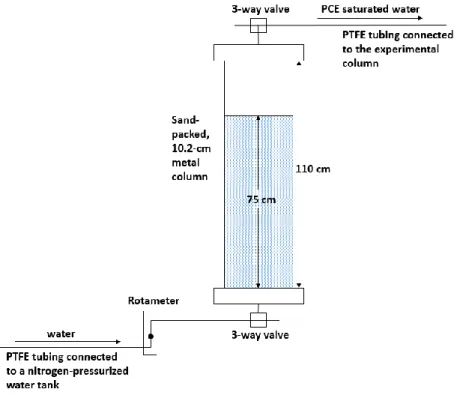
2.1 Generator column ... 19
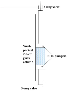
2.2 Experimental column ... 21
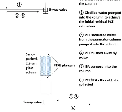
2.3 Procedures of PCE saturation experiments ... 24
2.4 The synthetic representation of the experimental porous medium constructed from a packing of 2,500 spheres with a porosity of 0.34 and a log radii variance of 0.2 ... 27
3.1 Tracer test results for HV3 and HV4 ... 32
3.2 Plot of the experimental data for the uniform sand column ... 34
3.3 Plot of the experimental data of HV1, HV2 and HV3 using PCE #1 ... 37
3.4 Plot of the experimental data of HV4 using PCE #2 ... 38
3.5 Plot of the experimental data of HV4 using SA-saturated PCE #3 ... 38
3.6 Plot of the experimental data of all columns using different PCE ... 39
3.7 Plot of experimental and simulation data of PCE #1 ... 41
3.8 Plot of normalized experimental and simulation data of PCE #1 ... 41
3.9 Plot of experimental and simulation data of PCE #2 ... 42
3.10 Plot of normalized experimental and simulation data of PCE #2 ... 42
3.11 Plot of experimental and simulation data of SA saturated PCE #3 ... 43
3.12 Plot of normalized experimental and simulation data of SA saturated PCE #3 ... 43
4.1 NAPL entrapped in porous media. At left, a 2D image of NAPL droplets in a porous medium system. At right, a 3D representation of a single NAPL droplet ... 45
4.2 Plot of saturation (non-normalized) vs NT for experiments ... 49
ix
1
CHAPTER 1: INTRODUCTION 1.1 Groundwater System
Groundwater refers to water that is found beneath the Earth’s surface, filling in the cracks and pores in soil, sand, and rocks. As a part of the water cycle, groundwater is recharged from natural sources, including deep percolation from precipitation, seepage from streams and lakes, and groundwater flows in the subsurface, and it may eventually discharge into surface waters such as streams and lakes [1, 2].
Subsurface water can be divided vertically into zones depending on the relative proportion of the pore space occupied by water: a zone of aeration, in which the pores contain both gases and water, and a zone of saturation, in which all pores are completely filled with water. The saturated zone is bounded above by a surface called water table, on which the pressure of the water is atmospheric. In groundwater hydrology, the term groundwater is often used to denote, in particular, water in the zone of saturation [3].
Groundwater makes up 1.7% of the total water on earth, while ground freshwater makes up 0.76% of total water, which is 30.1% of total freshwater [4]. Groundwater is often withdrawn for agricultural, municipal, and industrial use and provides the largest source of usable water storage in the United States [6]. According to U.S. Geological Survey (USGS), the United States
2
determined that 44% of the U.S. population depends on groundwater for its drinking water supply [27].
In a groundwater systems, flow takes place through a porous medium, which is defined as a system that consists of a continuous solid skeleton and a connected pore space that allows one or more fluids to flow through it [9]. A porous medium is characterized by morphology which includes geometric properties such as particle or pore shape and volume, and topology such as pore interconnectivity [35]. Porous medium flow is classified as single-phase, or two-phase, or multiphase depending on the number of immiscible fluid phases involved [9]. Compared to rivers and lakes, transport in porous media is generally slow and spatially variable due to heterogeneities in the medium [8]. The movement of groundwater is influenced by porosity, permeability, gravity, and pressure gradients. Mathematically, the velocity of groundwater flow can be described by Darcy’s law which will be introduced in Section 1.3.1. Processes that occur routinely in porous medium systems can be described mechanistically using the fundamental equations of mass, momentum, and energy conservation [9].
1.2 Groundwater Contamination
Groundwater contamination may be defined as the artificially induced degradation of natural groundwater quality [11]. A wide variety of contaminants from a large number of sources can cause degradation of groundwater quality, ranging from petroleum products to microbial
pathogens. A complete list and illustration of groundwater contamination types and sources will be presented in Section 1.2.2 and Section 1.2.3 respectively.
3
continue to migrate downward into groundwater), direct migration (contaminants migrate directly into groundwater from below ground sources), interaquifer exchange (contaminated groundwater mixes with uncontaminated groundwater), and recharge from surface water [18]. Soil can filter particulate matter out of water during infiltration but dissolved chemicals can still make their way into groundwater. Through these four ways, contaminants can occur in large enough concentrations in groundwater to cause problems and can be very difficult and costly to remediate [15].
The main groundwater contaminants of concern include petroleum hydrocarbons such as benzene, toluene, and xylene; chlorinated organics such as tetrachloroethylene (PCE),
trichloroethylene (TCE) and its associated daughter products; heavy metals such as lead, zinc, and chromium; and certain inorganic salts [16]. Some of these contaminants are soluble and will dissolve readily in water (i.e. hydrophilic), in contrast, other contaminants are less soluble in water (i.e. hydrophobic). Many contaminants we wish to remove from water are hydrophobic, particularly when the hydrophobic contaminant is present as a separate liquid phase, it is referred as a non-aqueous phase liquid (NAPL).
1.2.1 NAPL
4
such as gasoline and some industrial solvents, are less dense than water, and will tend to float on the water table [16, 29, 30].
NAPL droplets are trapped in porous media when capillary forces are greater than the mobilizing forces acting on the drop [33, 34]. Capillary forces make it extremely difficult or impossible to remove all the NAPL that have been released to the subsurface. For example, in petroleum recovery operations, pumping alone typically removes less than one-third of the oil in a petroleum reservoir, and even enhanced techniques such as water flooding or the application of surfactants can bring only 50% to 80% of the NAPL to the surface under optimum conditions. These recovery rates are acceptable to the oil industry. However, removal of much more than 99% of NAPL is probably required in order to restore a contaminated aquifer to drinking water standards, which is impractical without developing remediation technologies [17]. Rao et al. (1997) conducted a field-scale in situ cosolvent flushing at Hill Air Force Base in Utah to remove more than 85% NAPL [14]. Mulligan et al. (2001) wrote a review on
surfactant-enhanced NAPL remediation, which included 22 field experiments, only one of them reported a recovery rate of 99%, most of them reported a recovery rate between 80% and 90% [13]. 1.2.2 Types of Contamination
Based on different chemical compositions, groundwater contamination can be classified into six major types: (1) radionuclides, (2) tracer elements, (3) nutrients, (4) other inorganic species, (5) organic contaminants, and (6) microbial contaminants.
5
heavy metals such as lead, cadmium, chromium and mercury, derive from mining effluents, industrial waste water, agricultural wastes and fossil fuels. These toxic substances can
accumulate inside human bodies and may potentially be lethal. Nutrients are referred to as ions or organic compounds containing nitrogen or phosphorous. They result from agricultural practice including the use of fertilizers, cattle feeding and sewage, can cause methemoglobinemia and form carcinogenic compounds. Other inorganic species include metals present in non-trace quantities such as Ca, Mg, and Na plus nonmetals such as Cl and F, which originate from saline brine, mining, sanitary landfills and industrial waste water. These are generally not harmful, but exposure to high concentrations, especially Na, may disrupt cell and blood chemistry. Organic contaminants include chlorinated organics (such as PCE and TCE), petroleum hydrocarbons (such as benzene, toluene, and xylene), and pesticides which result from petroleum extraction, industrial and agricultural waste water. They can cause various kinds of health problems
including caner, liver damage, and brain disorders. Biological contaminants including pathogenic bacteria, viruses, or parasites, which come from human and animal sewage or waste water, can cause serious health conditions such as typhoid fever, cholera, polio and hepatitis [62].
1.2.3 Sources of Contamination
Sources of groundwater contamination are widespread. Examples include thousands of accidental spills, landfills, surface waste ponds, above or under-ground storage tanks, pipelines, injection wells, land application of waste and pesticides, septic tanks, radioactive waste disposal sites, salt water intrusion, and acid mine drainage, etc [16].
6
designed to store, treat, and/or dispose of substances; (3) discharge through unplanned release, e.g., landfills, surface impoundment, above or under-ground storage tanks and radioactive waste disposal sites; (4) sources designed to retain substances during transport or transmission, e.g., pipelines; (5) sources discharged as consequence of other planned activities, e.g.,
pesticide/fertilizer applications and mine drainage; (6) sources providing conduit or inducing discharge through altered flow patterns, e.g., production wells; and (7) naturally occurring sources whose discharge is created and/or exacerbated by human activity, e.g., salt water intrusion [16, 62].
In practice, the terms point and nonpoint are used to describe the degree of localization of the source. A point source is characterized by the presence of an identifiable, small-scale source, such as a leaking storage/septic tank, a disposal pond, a sanitary landfill or an accidental spill. In contrast, a nonpoint source is characterized by large-scale, relatively diffuse contamination originating from many smaller sources. Infiltration from farm land treated with pesticides and fertilizers is an example of a non-point source [62].
1.2.4 Remediation Methods
Many remediation methods, including physical and chemical remediation methods and bioremediation methods, are available to treat groundwater contamination. The most common remediation technologies are pump and treat, in situ air sparging, in situ flushing, permeable reactive barriers, and bio-based technologies.
7
at numerous sites for many years, through which their performances have been evaluated and the results have shown that it is not very effective at cleaning up contaminated sites because it takes a very long time (years to decades, depending upon local factors, contaminants, and cleanup standards) and can require a large volume of water to remove a majority of contaminants [63, 64, 65, 66]. In addition, it is especially inefficient for certain situations, such as those with
significant accumulations of DNAPLs trapped below the water table in heterogeneous media [63]. Due to its limitations, the pump-and-treat method is now primarily used for free product recovery and control of contaminant plume migration [19].
In situ flushing is the injection or infiltration of an aqueous solution (can be plain water, surfactant or cosolvent) into a zone of contaminated soil/groundwater via injection wells, followed by downgradient extraction of groundwater and above-ground treatment before discharge or re-injection [19, 67]. In situ flushing is designed to enhance conventional pump-and-treat by greatly reducing the time and amount of water used by mobilizing the sorbed contaminants. It is applicable to a wide variety of contaminants, and is not limited to the
contaminant depth or location within the hydrogeological regime [67]. The effectiveness of this method depends strongly on the ability of the solution to desorb, solubilize, and/or flush the contaminants.
Other remediation methods like in situ air sparging and permeable reactive barriers are not within the scope of related knowledge of this research. During the implementation of air sparging, a gas is injected into saturated soil zone below the lowest known level of
8
reactive material placed across the path of a contaminant plume. It either removes or degrades contaminants as contaminated water passes through it [19].
Choosing a remedial technology is a function of the type of contaminant, site hydrogeology, source characteristics, and the location of the contaminant in the subsurface. Among those factors, the variation of hydraulic conductivity or transmissivity of a formation is one of the most important parameters of interest [16].
1.3 Single-phase Flow 1.3.1 Darcy’s Law
Single-fluid-phase flow through a porous medium system is typically defined using Darcy’s law. Darcy’s law, first determined experimentally and reported by Henry Darcy in 1856 [10], is an equation that relates fluid pressure to flow rate in porous medium systems. It states that the volumetric flow rate through a column of porous material (Q) is proportional to the head loss across the sand column (h2-h1) and the cross-sectional flow area (A) and inversely proportional to the packed height of the column (L) [42], which can be written as
2 1
h h
Q KA
L
of which the differential form is expressed as
dh
Q KA
dL
where a minus sign has been introduced because flow is in the direction of decreasing head. In these two algebraic expressions, K is referred to as the hydraulic conductivity, which serves as a measure of the permeability of the porous medium with [11, 42]
k g
K
9
where k is the intrinsic permeability, which is determined for each porous medium system and depends on the distribution of the sizes, shapes, and orientations of the pores that provide pathways for flow within the solid system (i.e., the morphology and topology of the pore space) [42], ρ is the fluid density, g is the magnitude of the gravity vector and μ is the dynamic viscosity of the fluid.
The specific discharge, or Darcy velocity, can be written as:
Q q
A
The average macroscale pore velocity is related to the specific discharge by
q v
where α is the effective porosity.
Additionally, for single-phase, three-dimensional flow through an isotropic medium where a body force per unit volume is present, the Darcy’s law is typically expressed as
( )
k
p
q g
where q is the volumetric flow rate per unit area vector and g is the gravity vector. 1.3.2 Darcy-Forchheimer Law
10
2
dp
q q
dx k
where β is called the Forchheimer coefficient. 1.3.3 Reynolds Number
In a high velocity regime where the inertial effects become important, the flow begins to transition from Darcy flow to Forchheimer flow. Hence, criteria to identify the beginning of non-Darcy flow and the range of validity of non-Darcy’s law are needed. One of these criteria is the Reynolds number (Re). Re, which is named after Osborne Reynolds, serves as a criterion to help predict similar flow patterns in different fluid flow situations [39, 73]. It is physically the
dimensionless ratio of the inertial force to the viscous force [11], which is given by
Re
vL
where ρ is the density of the fluid, v is the (average) fluid velocity, L is a characteristic linear dimension, which is the mean grain size in porous media, and μ is the dynamic viscosity of the fluid.
According to Todd (2005), experiments show that Darcy’s law is valid for Re < 1 and is generally accurate up to Re = 10 [47], thus he determined Re = 10 as the upper limit to the validity of Darcy’s law [11]. However, it is not an exact value. Zeng (2006) concluded that the critical Re may range from 1 to 100 based upon a comprehensive review of the literature [44].
For Darcy-Forchheimer law, Irmay (1958) reported that at low Re (Re < 1), the inertia term of the Forchheimer equation may be neglected, at medium Re (1 < Re < 100), the inertia term is of same order as the first term, at larger Re (Re > 100), the inertia term gradually becomes
11 1.4 Multiphase Flow
1.4.1 Interfacial Tension and Contact Angle
Interfacial tension (IFT) and contact angle are two important properties to describe a
multiphase system. IFT is defined as the free surface energy at the interface formed between two immiscible fluids [68]. It is caused by the unbalanced forces of liquid molecules at the surface and the tendency of the liquid to maintain the lowest surface free energy. IFT is responsible for the shape of liquid droplets, which tends to be a sphere. Thus, IFT can be measured by analyzing the shape of the drop. Several methods currently used to measure IFT are based on this principle. The most commonly used one is the pendant drop method where the actual shape of a hanging drop is matched to theoretical simulations to compute the IFT [69, 70]. Liquid IFT is directly related to the capillary pressure (introduced in Section 1.4.3) across an NAPL-water interface and is a factor controlling wettability [49].
The contact angle is defined as the angle between the solid surface and the fluid-fluid interface and is usually measured in wettability studies [32]. There are multiple conventions with regard to measuring contact angles. A usual convention is to measure the angle through the bulk phase (as opposed to measuring through the drop). In this convention, large contact angles (>> 90°) correspond to high wettability with regard to the bulk fluid, and the drop will spread over a large area on the surface; while small ones (<< 90°) correspond to low wettability and the drop tends to minimize its contact with the surface and form a compact liquid droplet. Contact angle is, like IFT, related to the capillary pressure as well, and is actually defined in terms of IFT according to Young’s Formula [68].
1.4.2 Darcy’s Law for Multiphase Flow
12 ( ) k p q g
For each phase in a multiphase flow, this equation can be directly extended to multiphase flow [48]. For phase α,
( ) k p q g
where α indicates that the physical quantity is for phase α.
The effective permeability for each phase is not greater than the intrinsic permeability k of the porous medium with [48]
r
k k k
where krα is the relative permeability which indicates the tendency of phase α to wet the porous medium.
Therefore, for phase α, Darcy’s equation can also be written in terms of krα and k as
( ) r k k p q g
1.4.3 Capillary Pressure
When two immiscible fluids are in contact inthe pores of a porous medium, a pressure
difference exists across the interface separating them. This pressure difference is called capillary pressure and is related to the IFT and curvature of the interface [3, 50]. The capillary pressure causes porous media to draw in the wetting fluid and repel the non-wetting fluid [49].
At the macroscale, capillary pressure is the product of average IFT and the average interfacial curvature [51]:
c wn wn
w
13
wherepcis the average capillary pressure over the wn interface, wn is the average IFT over the
wn interface, and Jwwn is the macroscale surface curvature defined as the average over the wn
interface of the surface divergence of the outward normal from phase w. Particularly, at equilibrium, the capillary pressure is given as [51]:
c n w
p p p
where pn is the non-wetting phase pressure, and pw is the wetting phase pressure. This equation is not valid for a dynamic system.
Capillary pressure has been found to closely relate to saturation and permeability. Pressure-saturation-permeability(p-S-k) relations are of central importance of modeling multiphase systems. Modeling of p-S-k relations can be subdivided into: (1) pressure-saturation (p-S) models, (2) saturation-permeability (S-k) models, and (3) hysteresis models. Attempts have already been made to derive these models. Several empirical and semi-empirical expressions of these models are available in the literature [52]. For example, laboratory experiments have shown that capillary pressure can be represented as a function of saturation [53]. The Brooks-Corey (1964) and van Genuchten (1980) models are two well-known empirical models that relate the capillary pressure to the saturation of the phases [50, 54].
1.4.4 Capillary Number, Bond Number and Trapping Number
There are three important dimensionless numbers in entrapped NAPL mobilization: the capillary number (NCa), the bond number (NB) and the trapping number (NT). The capillary number represents the ratio of viscous forces to capillary forces, the bond number represents the ratio of the gravity/buoyancy to capillary forces, and they are combined to form NT with [33]:
2 2
2 sin
T Ca Ca B B
14
where α is the angle the flow makes with the positive x axis.
For vertical flow (α = 90°), in the direction of the buoyancy force, their expressions can be expressed as [33]:
cos l w w Ca ow q N , cos rw B ow gkk N
, and
2 2
2
cos
l
w w rw
T Ca Ca B B Ca B
ow
q gkk
N N N N N N N
respectively, where qwis the Darcy velocity of the aqueous phase, μw is the dynamic viscosity of
the aqueous phase, σow is the IFT between the organic liquid and water, θ is the contact angle, Δρ is the difference of the density between the aqueous phase and the organic phase, g is the gravity acceleration constant, k is the intrinsic permeability of the porous medium, krw is the relative
permeability to the aqueous phase.
NT quantifies the balance of gravitational, viscous, and capillary forces acting on an entrapped
15 1.5 Turbulence
In fluid dynamics, turbulence refers to a high velocity flow regime characterized by chaotic, stochastic property changes. The flow field of turbulence consists of a mean (time-averaged) component plus a random, chaotic motion [40].
A highly viscous or slow-moving fluid tends to be smooth and regular, which is called laminar flow. As the viscosity reduces, or the fluid velocity increases, the movement of the fluid becomes irregular and chaotic, which is called turbulent flow. This process is called the transition to turbulence and has been illustrated in a number of experiments such as Reynolds’ experiments [39, 40, 73]. Laminar flow admits a steady flow field and tends to flow without lateral velocity, which means there are no cross currents perpendicular to the direction of flow. Due to the
presence of lateral velocity, turbulent flow transports and mixes fluid much more effectively than a comparable laminar flow [39, 72]. During transition, the Re serves as a criterion to distinguish between laminar and turbulent flow. Laminar flow occurs at low Re where viscous forces are dominant, while turbulent flow occurs at high Re where inertial forces are dominant.
A steady state cannot be achieved when a flow is transitioning to the turbulent flow, due to the eddies that form in the system, the pressure field and the velocity field are constantly oscillating. These fields are three-dimensional, time-dependent and random, which makes it difficult to develop an accurate tractable theory or model. For a turbulence problem, there are no prospects of a simple analytic theory. Instead, hopes are placed on the use of ever-increasing power of digital computers [72].
16 1.6 Modeling Approaches
A wide range of spatial scales are used when describing porous medium systems. These scales, from the smallest to the largest, are referred to, respectively, as the molecular scale, the microscale, the resolution scale, the macroscale, and the megascale [9]. Models may be
developed at different length scales and are associated with the scale being considered. Most common models are formulated at the microscale and macroscale.
The microscale, also referred to as the pore scale, is the scale at which all details of the
morphology and topology of the pore space and solid phase distribution are known, which means the location of each solid grain and the distribution of the fluid phases are resolved in space and time. At this scale, the length scale of the fluid system is much larger than that of a single molecule or its mean free path, and hence the fluid is considered as a continuum [7, 61].
The macroscale is the scale at which the details of the microscale are not available and a point represents the averaged condition in a region around the point. At the macroscale, we work with averaged quantities, such as porosity, which describes the pore space available at the microscale; as well as fluid saturation and permeability to describe systems. By averaging, the intricate variations due to the microscopic heterogeneity are smoothed out, and the system can be considered as an equivalent homogeneous system.
17
At the microscale, the Navier-Stokes equation can be approximated using numerical methods. Instead of solving the Navier-Stokes equation, the lattice Boltzmann method (LBM) can be used to solve the discrete Boltzmann equation to simulate the flow of a Newtonian fluid with collision models [58, 37]. According to several reviews by Benzi et al. (1992), Chen et al. (1998) and Aidun et al. (2010), LBM has been applied to various flow conditions including
two-dimensional, three-dimensional turbulence, and multiphase flows through porous media [57, 58, 59].
Microscale modeling offers an important tool to understand pore-scale flow and transport processes that influence the macroscopic behavior. However, the modeling approaches are computationally intensive and are not feasible to be used to simulate a system where the
characteristic length is on the order of meters or longer. Therefore, upscaling approaches such as thermodynamically constrained averaging theory (TCAT) are implemented to manifest the microscopic processes at larger spatial scales [9, 12].
1.7 Research Objectives
18
CHAPTER 2: EXPERIMENTAL METHODS 2.1 Experimental Materials
All reagents used, including isopropanol (IPA), tetrachloroethylene (PCE), acetonitrile, and dibenzothiophene (DBT), were ACS reagent grade or better. A 12/20 mesh Accusand (d50 =
1.105 ± 0.014 mm, uniformity coefficient = 1.231 ± 0.043, ρ = 2.655 g/cm3, hydraulic
conductivity = 0.503 ± 0.017 cm/s) and a polydisperse sand mixture composed of 11 different grain sizes ranging from 0.35 mm to 3 mm and following a log-normal particle size distribution with a mean diameter of 1.15 mm and a variance of 0.52 mm, were used in the column
experiments.
19 2.2 Column Experiments
2.2.1 Generator Column
A generator column composed of a large metal column with 10.2-cm inner diameter and 110 cm total length was used to generate PCE-saturated water for the experimental column. The column was filled with 75 cm of 12/20 Accusand, which had a porosity of 0.43. The total pore volume of the column was calculated by adding the volume of the unfilled part and the pore volume of filled part, which was found to be 5.5 L. The inlet of the generator column was connected to a nitrogen-pressurized water tank with polytetrafluoroethylene (PTFE) tubing. A rotameter was installed between the water tank and the generator column to allow control of the flow rate. The water in the tank was driven by the pressure created by a compressed nitrogen tank, and entered the generator column through the PTFE tubing. As the water flowed upward through the generator column, the solution became saturated with the PCE that was entrapped in the porous medium. The generator column setup is shown as Fig 2.1.
20
After the column was packed with sand, dyed PCE was then injected into the column from the bottom, then water was flushed upward through the column at 1500 mL/min to make sure the PCE was dispersed evenly within the sand and any mobile PCE was removed. Once no visible PCE eluted from the column, the effluent was collected and the concentration of dissolved PCE was measured using high-performance liquid chromatography (HPLC). The results were
averaged and compared with the result from a batch test to determine if the effluent from the generator column had been saturated with PCE. The batch test involved mixing PCE with distilled water at a 1:5 volume ratio in three centrifuge tubes, shaking for over 12 hours, and measuring the dissolved PCE concentration by HPLC to determine the solubility of PCE in distilled water.
2.2.2 Experimental Column
21
Fig 2.2: Experimental column
Each plunger contained a 0.45-cm inner diameter tubing that was connected to a three-way valve. Two programmable syringe pumps (Harvard Apparatus PHD 4400) were used to inject PCE, IPA and distilled water.
One uniform sand column packed with 12/20 Accusand and four high-variance sand columns (HV1, HV2, HV3 and HV4) packed with a polydisperse sand and a glass bead mixture with a log normal grain size distributionwere packed during the course of the experiment work. For each of the columns, the length of the filled column was measured, and the mass of media added to the column was divided by the particle density of the porous medium to calculate the solid volume of the column. The pore volume was then determined by subtracting the solid volume from the total volume. Additionally, the porosity of the column was calculated by dividing the pore volume by the total volume of the column.
After the column was packed with porous media, CO2 was then pumped through the column
22
upwards, at a rate of 20 mL/hr to displace the CO2, until 10 pore volumes of water was moved
through the system. 2.2.3 Tracer Tests
A series of tracer tests were performed on the experimental columns using a stock solution of tritiated water (T2O), a radioactive form of H2O where the hydrogen atoms are replaced with
tritium (3H or T). The results of the tracer tests were used to identify if there was significant flow by-passing in a specific column packing during flushing.
Initially, T2O was pumped upwards through the column at a flow rate of 10 mL/hr. Samples
were collected in 20-mL plastic scintillation vials, which were numbered and weighed prior to the experiment. Samples were taken every 2.5 mL, or every 15 minutes, until more than 2.5 pore volumes of the experimental column had been pumped through the column in order to ensure that the distilled water in the experimental column was completely replaced with T2O. The filled
sample vials were then weighed again and mixed with 7.5 mL of scintillation cocktail (ScintiSafe 30% LSC-Cocktail) and analyzed on a scintillation counter (Packard 1900 TR Liquid
Scintillation Analyzer) to determine the disintegrations per minute (DPM). Finally, this value for each sample was divided by the volume of the sample to find DPM per mL.
2.2.4 PCE Saturation Experiments
A series of specific flushing experiments were conducted on the experimental column to reveal the relationship between the flow rate of flushing and the entrapped saturation of PCE. Increasing the flow rate of water, increases the mobilizing viscous forces acting on the entrapped organic phase.
23
24
Fig 2.3: Procedures of PCE saturation experiments
For each column packing, a number of measurements of the PCE saturation after the 20mL/hr flow rate step were made to determine the initial residual PCE saturation and to make sure all the experiments had a similar initial state of PCE saturation.
2.3 Analytical Methods 2.3.1 Interfacial Tension
IFT was measured using the pendant drop method. A polycarbonate cuvette was filled with distilled water (pre-equilibrated with PCE), and a drop of PCE was suspended from a stainless steel needle. A digital video camera captured images of the drop, and Kruss’s Drop Shape Analysis II (DSA2) software was used to determine the native IFT. IFT measurements were conducted using dyed (Oil-red-o) PCE.
25
centrifuging to separate the phases. Between each sample, the plastic cell was replaced with a new one.
2.3.2 Contact Angle
Contact angles were measured using the same instrumentation and software that were used for the IFT measurements. A drop was dispensed by needle on a 25 × 25 mm quartz slide
(Chemglass) placed in the glass cell, then images were captured to measure the static (θS) contact angles (through the aqueous phase) on each side of the drop.
An inclined plate method was used to measure the advancing (θA) and receding (θR) contact angles, where exactly same steps were followed but the stage was tilted until the drop just began to move along the surface of the slide and images were captured immediately prior to the
movement of the drop.
Contact angle measurements were conducted with the equilibrated PCE and aqueous phases. Between each sample, the glass cell and quartz slides were rinsed sequentially with acetone, methylene chloride, and acetone again, followed by a final, thorough distilled water rinse. 2.3.3 PCE Analysis
2.3.3.1 PCE Extraction
Effluent samples from the column experiments were collected in centrifuge tubes. The
26 2.3.3.2 HPLC Methods
Analysis was performed by HPLC (Water 600S controller, 616 pump, and 717 autosampler) equipped with a WatersTM 996 Photodiode Array Detector, a Thermo Scientific Hypersil Green PAH column (10 cm × 4.6 mm, 3 um packing), and HPLC grade solvents. The HPLC method used an isocratic flow program using 30% water, 70% acetonitrile at 1.00 mL/min. Both PCE and the internal standard, DBT, were measured at a wavelength of 223.0 nm.
2.3.3.3 Calibration Curves
PCE was quantified by HPLC using an internal standard method. Calibration was performed with six standard solutions containing PCE in concentration from 200 to 2000 mg/L, along with the internal standard. The PCE stock solution was made by dissolving 1 g PCE solution into a 100 mL IPA. The exact weight of PCE was measured and recorded. Then a series of PCE calibration solutions was made in a 10-mL volumetric flasks from the 100-mL stock solution. The data points were fitted to a linear equation that was used to calculate the concentration of PCE in experimental samples. All the calibration curves had an R2 > 0.99 to ensure accuracy. PCE calibration curves for HPLC were made and updated every 2-3 weeks, in order to ensure the accuracy of the experiments.
2.3.4 Lattice Boltzmann Methods
Mobilization simulations matching the experimental conditions were carried out using a three-dimensional, 19-velocity-vector (D3Q19), multiple-relaxation time (MRT) lattice Boltzmann method [23]. A three-dimensional, synthetic representation of the porous medium used in the laboratory experiments was generated using a sphere packing algorithm [24]. The porosity and lognormal size distribution for the sphere radii of the sphere pack were set to match the
27
in a non-overlapping fashion with a porosity of 0.34 and a log radii variance of 0.2, as shown in Fig 2.4. The lattice size necessary to achieve a grid-independent solution was 5203, which
corresponded to a 0.04-mm grid resolution.
Fig 2.4: The synthetic representation of the experimental porous medium constructed from a packing of 2,500 spheres with a porosity of 0.34 and a log radii variance of 0.2. In the LBM three parameters must be established: ζ, which controls the interfacial width, σ, which determines the IFT γwn, and φs, which controls the contact angle θ. A ζ of 0.9 was used based on previous analysis that concluded the parameter is independent of IFT. The parameters σ
and φs were determined to match the experimental parameters using a bubble test in the absence
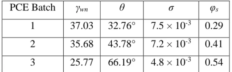
of the solid phase and a constrained bubble test, respectively, as described in Dye et al. (2015) [25]. Table 2.1 lists the determined values for σ and φs for each experimental porous medium system.
PCE Batch γwn θ σ φs
1 37.03 32.76° 7.5 × 10⁻³ 0.29 2 35.68 43.78° 7.2 × 10⁻³ 0.41
3 25.77 66.19° 4.8 × 10⁻³ 0.54
28
The initial conditions for the mobilization simulations were determined by simulating drainage and imbibition in the synthetic porous medium systems outlined in Table 2.1. A displacement simulation began with a fully wetting-phase-saturated system. Constant pressure boundary conditions were set on one face for one fluid and on the opposite face for the second fluid, with no-flow boundaries on all other boundaries. The simulation was performed by varying the pressure boundary conditions and allowing the system to reach an equilibrium state before the next step change in fluid pressures, where equilibrium was determined by the change in
interfacial curvature. The microscale fluid density distribution was obtained for each equilibrium state and used to identify the regions of the pore-space occupied by the wetting (w) phase domain
Ωw, the non-wetting (n) phase domain Ωn, and the wetting-non-wetting (wn) interfacial domain
Ωwn. All the phases and interfaces could be identified explicitly because the position of the solid
(s) phase was known. After each entity was identified, the saturation of the non-wetting phase was computed according to
1
1 k n
k w n n
s
XXwhere Xk denotes lattice site k. The state of the system at the end of imbibition was used as the initial condition for the mobilization simulations for a given synthetic porous medium system. In the mobilization simulations, a constant velocity boundary condition was set on the inlet face and a periodic boundary condition on the outlet face of the system, with no-flow boundaries on all other boundaries. The velocity boundary condition on the inlet was set to match the
29
30
CHAPTER 3: EXPERIMENTAL RESULTS 3.1 PCE Properties
3.1.1 PCE solubility in distilled water
The solubility of PCE in distilled water was found to be 190 ± 20 mg/L in the batch test. Comparing this concentration with reported values in the literature tested the validity of the method. Gillham (1990) reported the solubility of PCE is 200 mg/L at 20°C [79]. Ladaa et al. (2000) measured the solubility of PCE in deionized water at 25°C, which was reported to be 215 ± 20 mg/L [21]. Mackay et al. (1993) quoted the measured solubilities of PCE in water to range from 150 up to 489 mg/L, which were determined using a variety of experimental methods [22]. These literature values are consistent with the measured value.
3.1.2 Interfacial Tension and Contact Angle
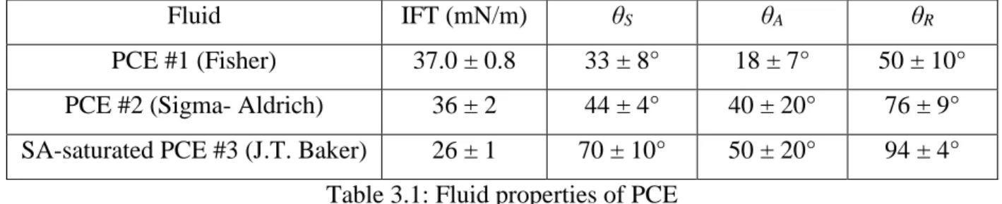
The fluid properties of the three different batches of PCE are summarized in Table 3.1.
Fluid IFT (mN/m) θS θA θR
PCE #1 (Fisher) 37.0 ± 0.8 33 ± 8° 18 ± 7° 50 ± 10° PCE #2 (Sigma- Aldrich) 36 ± 2 44 ± 4° 40 ± 20° 76 ± 9° SA-saturated PCE #3 (J.T. Baker) 26 ± 1 70 ± 10° 50 ± 20° 94 ± 4°
Table 3.1: Fluid properties of PCE
31
close to each other, while SA-saturated PCE #3 had a much larger θS (70°) than PCE #1 and PCE #2.
Since the value of IFT depends strongly on the temperature, the measuring method and the instrumentation used, the literature values for the IFT between PCE and water vary, but the reported values are mostly higher than 43 mN/m [33, 77, 78, 82]. Despite careful and thorough cleaning of the instrumentation and repeated experimentations, the measured IFT remained lower than those literature values. However, Gioia (2006) reported an IFT of 36.5 mN/m for PCE [83], which is much closer to the measured IFT.
The reduction of the interfacial tension in SA-saturated PCE #3 is due to the affinity of the SA (a surfactant) for both hydrophilic and hydrophobic molecules [74]. The ability of SA to
decrease IFT between the NAPL and aqueous phase has also been reported in other studies [75, 76].
3.2 Column Experiments
3.2.1 Parameters for Column Packings
Table 3.2 shows all the parameters for each column, including the column length, packing material, pore volume and porosity.
Column name Column length (cm)
Packing material
Pore volume (mL)
Porosity
Uniform sand column 5.18 12/20 Accusand 8.52 0.335
HV1 7.78 A polydisperse
sand and glass bead mixture
12.8 0.336
HV2 7.42 12.2 0.334
HV3 8.02 14.0 0.356
HV4 7.65 14.4 0.383
32 3.2.2 Tracer Test Results
The results of the tracer tests can be seen in Fig 3.1, which shows the results for gradually replacing distilled water with T2O in HV3 and HV4, where the x-axis represents the ratio of the
injected volume of T2O to the pore volume of the system (the sum of the pore volume of the
experimental column and the total volume of the tubing between the outlet and the pump) and the y-axis represents the ratio of the T2O concentration to the injected concentration. The time
for each test was started when the syringe pump was started.
Fig 3.1: Tracer test results for HV3 and HV4
In Fig 3.1, both curves are reasonably symmetric and there is no evidence of significant flow by-passing in these two column packings.
3.2.3 Uniform Sand Column Results
A set of preliminary experiments was conducted with a column packed with 12/20 Accusand using PCE #1. At the beginning of the experiment, the PCE saturation in the experimental
column approached 100%. Most of the PCE was removed during the 20 mL/hr water flush. After that stage, the rest of PCE were evenly dispersed as droplets in the experimental column. Then
0 0.2 0.4 0.6 0.8 1 1.2
0 0.2 0.4 0.6 0.8 1 1.2 1.4 1.6 1.8
R ati o of n or m al iz e d T2 O co n cen tr ati on
Pore Volume of injected T2O
33
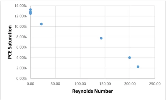
during the high Re flushing, the PCE droplets were removed from the column rapidly after flushing began. Additional PCE-saturated water was pumped through the experimental column to ensure that steady-state had been reached. The residual remaining after flushing visually decreased as the Re number was increased. In very high Re flushing where Re > 200, nearly all visible PCE was mobilized from the experimental column. The experimental data of the PCE saturation experiments of the uniform sand column are shown in Table 3.3, and a plot of the results is shown in Fig. 3.2.
Re PCE saturation 0.04 13.25% 0.04 12.78% 0.04 12.77% 0.04 12.51% 22.0 10.48% 142.3 7.75% 199.4 4.01% 216.2 2.26%
34
Fig 3.2: Plot of the experimental data for the uniform sand column
In the uniform sand column experiment, a near linear decrease in the residual saturation was observed as Re increased, as seen in Fig 3.2. The PCE saturation finally ended up around 2% at an Re of 220.
A problem with the uniform sand column was that the sphere packing program used to generate the medium for the lattice Boltzmann simulations was unable to precisely match the experimental column. Therefore, a column medium consisting of a polydisperse sand and glass bead mixture with a log normal grain size distribution was produced and used to pack subsequent columns as discussed in the next section.
3.2.4 High-Variance Sand Column Results
A series of PCE saturation experiments were conducted with four different columns (HV1, HV2, HV3 and HV4) packed with the same polydisperse sand and glass bead mixture with a log normal grain size distribution using three different batches of PCE. The experimental
observations of the high-variance sand columns were generally similar to those of the uniform sand column.
0.00% 2.00% 4.00% 6.00% 8.00% 10.00% 12.00% 14.00%
0.00 50.00 100.00 150.00 200.00 250.00
PCE
Sa
tu
ra
ti
on
35
First, a series of PCE saturation experiments were conducted on HV1, HV2 and HV3 using PCE #1. For PCE #1 in HV1, HV2 and HV3, the average initial saturations (after 20 mL/hr distilled water flushing) were 7.7 ± 0.4%, 8 ± 1% and 8 ± 2% respectively. These concentrations served as the starting points for the subsequent high Re experiments.
Next, a series of PCE saturation experiments were performed on HV4 using PCE #2, which had a slightly lower IFT and higher contact angle than PCE #1. The average initial saturation was 10.7 ± 0.8%. This initial residual PCE saturation of PCE #2 was higher than that of PCE #1. Finally, a series of PCE saturation experiments were carried out on HV4 using SA-saturated PCE #3, which had significantly lower IFT and higher contact angle than PCE #1 and #2. The average initial saturation was 11.9 ± 0.5%. This initial residual PCE saturation of SA-saturated PCE #3 was higher than those of both PCE #1 and PCE #2.
36
Re PCE saturation Re PCE saturation Re PCE saturation PCE #1 HV1
0.04 7.33% 0.04 7.54% 0.04 8.17%
0.04 7.52% 0.04 8.01% 113.1 6.24%
143.3 3.14% 243.2 0.99%
PCE #1 HV2
0.04 7.85% 0.04 8.54% 0.04 8.70%
47.4 6.25% 53.0 7.09% 102.2 6.53%
143.0 4.20% 179.0 2.56% 252.5 0.86%
PCE #1 HV3
0.04 9.03% 0.04 7.73% 0.04 7.69%
160.2 4.17% 167.8 2.74% 203.7 1.94%
228.8 0.95% 250.0 1.43% 271.0 0.95%
PCE #2 HV4
0.04 10.50% 0.04 10.59% 0.04 11.13%
28.3 9.46% 53.0 8.57% 76.9 6.88%
101.8 6.54% 128.6 4.14% 149.6 3.42%
172.4 2.03% 189.4 1.82% 215.4 1.08%
SA-saturated PCE #3 HV4
0.04 11.56% 0.04 11.83% 0.04 11.92%
0.04 12.37% 29.0 10.36% 30.2 10.38%
58.9 9.46% 73.5 7.73% 82.4 7.60%
98.9 5.47% 123.4 4.09% 131.2 4.18%
138.6 2.35% 153.4 1.91% 155.4 1.74%
170.7 1.59% 174.0 1.67% 191.2 1.28%
214.7 0.80% 223.3 0.79%
37
All PCE #1 experimental data, grouped by different columns, are shown below in Fig 3.3. As seen in Fig 3.3, the saturation of PCE #1 decreased roughly linearly through an Re of 250, but the saturation data showed a relatively high variability at low Re regime.
Fig 3.3: Plot of the experimental data of HV1, HV2 and HV3 using PCE #1
For the experiments conducted with PCE #2, the PCE saturation decreased almost linearly as Re was increased to about 225, as seen in Fig 3.4. The PCE saturations of PCE #2 were
considerably higher than those of PCE #1 (Fig 3.3) in the low Re regime, however, the differences between PCE #1 and PCE #2 saturations began to decrease as Re increased. The saturations for both PCE #1 and PCE #2 were around 1% at Re > 220.
0.00% 1.00% 2.00% 3.00% 4.00% 5.00% 6.00% 7.00% 8.00% 9.00% 10.00%
0 50 100 150 200 250 300
PCE
sa
tu
ra
ti
on
Reynolds Number
HV1
HV2
38
Fig 3.4: Plot of the experimental data of HV4 using PCE #2
The plot of SA-saturated PCE #3 shown below in Fig 3.5 resembles a hockey stick. The saturation of SA-saturated PCE #3 decreased roughly linearly through an Re of 150, then the trend became much flatter through an Re of 220. SA-saturated PCE #3 displayed higher
saturations relative to prior two batches of PCE in the low Re regime, and the differences began to decrease as Re increased. The saturation of SA-saturated PCE #3 was around 0.8% at an Re of 220, which was very close to PCE #1 and PCE #2.
Fig 3.5: Plot of the experimental data of HV4 using SA-saturated PCE #3
0.00% 2.00% 4.00% 6.00% 8.00% 10.00% 12.00%
0 50 100 150 200 250
PCE sa tu ra ti on Reynolds Number 0.00% 2.00% 4.00% 6.00% 8.00% 10.00% 12.00%
0 50 100 150 200 250
39
Fig 3.6 shows all the plots in a single picture, where all the initial saturations were averaged to show only one starting point.
Fig 3.6: Plot of the experimental data of all columns using different PCE 3.3 Lattice Boltzmann Results
Lattice Boltzmann simulations were conducted for a system corresponding to the high-variance sand columns to compare with experimental results. Since there was a discrepancy between the initial conditions of experimental data and those of simulation data, the saturation data were normalized by the initial residual saturation in order to make their initial conditions match. The simulated NWP saturations were always greater than the experimental data so the saturation data was normalized based on the initial residual saturation of simulated data.
The entrapped non-wetting phase saturation for each synthetic porous medium system is listed in Table 3.6, relevant plots are shown in Fig 3.7, Fig 3.8, Fig 3.9, Fig 3.10, Fig 3.11 and Fig 3.12. The upper limit of Re was 220.0 because when Re >220, the flow was transitioning to
0.00% 2.00% 4.00% 6.00% 8.00% 10.00% 12.00%
0 50 100 150 200 250 300
PCE
Sa
tu
ra
ti
on
Reynolds Number
PCE#1 HV1
PCE#1 HV2
PCE#1 HV3
PCE#2 HV4
40
turbulent flow and the pressure and velocity in the system became constantly oscillating, such that a steady state flow field could not be achieved. To capture all the physics in this regime, the system needs to be discretized even more and due to limited computing power that becomes difficult.
Re PCE saturation Normalized Re PCE saturation Normalized PCE #1
0.04 10.72% 100% 5.0 10.54% 98.32%
35.0 9.17% 85.54% 60.0 8.18% 76.31%
100.0 6.42% 59.89% 150.0 4.74% 44.22%
180.0 3.84% 35.82% 200.0 3.23% 30.13%
220.0 2.77% 25.84%
PCE #2
0.04 11.81% 100% 5.0 11.59% 98.14%
35.0 10.23% 86.62% 60.0 9.16% 77.56%
100.0 7.02% 59.44% 150.0 4.16% 35.22%
180.0 2.57% 21.76% 200.0 2.17% 18.37%
220.0 2.01% 17.02%
SA-saturated PCE #3
0.04 13.62% 100% 5.0 13.38% 98.24%
35.0 11.74% 86.20% 60.0 10.22% 75.04%
100.0 7.81% 57.34% 150.0 4.62% 33.92%
180.0 3.13% 22.98% 200.0 2.63% 19.31%
220.0 2.47% 18.14%
Table 3.5: Lattice Boltzmann simulation data
41
Fig 3.7: Plot of experimental and simulation data of PCE #1
Fig 3.8: Plot of normalized experimental and simulation data of PCE #1
A plot of experimental and simulation data of PCE #2 is shown below in Fig 3.9, followed by a plot of normalized data shown in Fig 3.10. As is expected, simulated residual saturations of PCE #2 were higher than those of PCE #1.
0.00% 2.00% 4.00% 6.00% 8.00% 10.00% 12.00%
0 50 100 150 200 250 300
PCE sa tu ra ti on Reynolds Number experiment HV1 experiment HV2 experiment HV3 simulation 0.00% 10.00% 20.00% 30.00% 40.00% 50.00% 60.00% 70.00% 80.00% 90.00% 100.00%
0 50 100 150 200 250 300
42
Fig 3.9: Plot of experimental and simulation data of PCE #2
Fig 3.10: Plot of normalized experimental and simulation data of PCE #2
According to Fig 3.9 and Fig 3.10, the simulation data of PCE #2 matched the experimental data much better than those of PCE #1. Similarly, simulation data decreased linearly as Re was increased to 180, then the trend became much flatter through an Re of 220.
0.00% 2.00% 4.00% 6.00% 8.00% 10.00% 12.00%
0 50 100 150 200 250
PCE sa tu ra ti on Reynolds Number experiment simulation 0.00% 10.00% 20.00% 30.00% 40.00% 50.00% 60.00% 70.00% 80.00% 90.00% 100.00%
0 50 100 150 200 250
43
A plot of experimental and simulation data of SA-saturated PCE #3 is shown below in Fig 3.11, followed by a plot of normalized data shown in Fig 3.12. Similar to PCE #2, simulation data of SA-saturated PCE #3 decreased linearly through an Re of 180, then the trend became much flatter through an Re of 220.
Fig 3.11: Plot of experimental and simulation data of SA saturated PCE #3
Fig 3.12: Plot of normalized experimental and simulation data of SA saturated PCE #3
0.00% 2.00% 4.00% 6.00% 8.00% 10.00% 12.00% 14.00%
0 50 100 150 200 250
P CE sa tu ra ti on Reynolds Number experiment simulation 0.00% 10.00% 20.00% 30.00% 40.00% 50.00% 60.00% 70.00% 80.00% 90.00% 100.00%
0 50 100 150 200 250
44
Overall, all simulation data decreased linearly through an Re of 180. Then, simulation data of PCE #2 and SA saturated PCE #3 became much flatter, resulting in a hockey-stick shape, which was however, not obvious for the results using PCE #1. Among all three batches of PCE,
45
CHAPTER 4: DISCUSSIONS 4.1 NAPL Mobilization Mechanisms
Before the experimental results are analyzed and discussed, NAPL mobilization mechanisms, from which the expressions of three significant dimensionless quantities (NCa, NB and NT) are derived, needs to be introduced.
In order to analyze NAPL mobilization mechanism, it is reasonable to start from a single NAPL droplet entrapped in a single pore in porous media. Fig 4.1 depicts a single NAPL droplet stuck in a pore volume. In the 2D slide, NAPL is depicted in color and the porous media is in black. In the 3D rendering, the red spheres represent the porous media and the green one represents the NAPL.
46
When a NAPL droplet is entrapped in a single pore in porous media, it is actually in a state of force balance within this pore, which is formally termed as the critical conditions for
mobilization. Under such conditions, mobilization forces balance retention forces. More specifically, viscous and gravity/buoyancy forces acting to mobilize the NAPL droplet, are balanced by capillary forces acting to retain the NAPL droplet.
By equating the balanced forces in the critical conditions and applying Darcy’s law to express the pressure gradient, Pennell et al. (1996) proved that the expression NCaNBsin could be
used to assess the potential for NAPL mobilization in a pore [33], where
cos l w w Ca ow q N
which
represents the ratio of the viscous to capillary forces,
cos rw B ow gkk N
which represents the ratio
of the gravity/buoyancy to capillary forces, α is the angle the flow makes with the positive x axis.
NCa and NB are used to quantify the contribution of viscous and gravity/buoyancy forces to
NAPL mobilization respectively, although alternative expressions for them exist [84, 85, 86, 87, 88, 89, 90], their functionalities remain unchanged.
The combined effect of NCa and NB is represented by NT and is expressed as [33]:
2 2
2 sin
T Ca Ca B B
N N N N N
By following the convention above for NCa and NB, for vertical flow (α = 90°), in the direction of the buoyancy force, the expression for NT becomes [33]:
2 2
2
cos
l
w w rw
T Ca Ca B B Ca B
ow
q gkk
N N N N N N N
47
This expression suggests that at low flow rates when NT is relatively small, NAPL droplets are trapped in the porous media by capillary force, whereas at high flow rate when NT is relatively large, capillary forces are overwhelmed by the viscous forces, which act to mobilize the droplet. 4.2 Comparison of Simulation and Experimental Results
First, the discrepancy between the simulation and experimental results must be addressed. It has already been shown in Section 3.3 that simulation data were always larger than experimental data, which can be observed from the initial residual saturation through the saturation under the upper limit of Re. This actually results from the fact that the simulated system, as presented in Section 2.3.4, was only an idealized representation of the experimental porous media rather than a realistic picture of the actual porous media. Therefore, it is reasonable to see the simulation and experimental results were not exactly same.
Next, the relationship between saturations and NT will be examined based on the theory described in Section 4.1. Data were obtained from column experiments and simulation results, plots were made with both normalized saturations and absolute ones. All the NCa, NB and NT results for both experiments and simulations are shown below in Table 4.1 and Table 4.2 respectively, and plots are shown in Fig 4.2, Fig 4.3, Fig 4.4 and Fig 4.5. The physical and chemical constants used in computing are listed as follows: the density of water: 0.998 g·cm–3 (22.0°C), the density of PCE: 1.623 g·cm–3 (20°C), μw: 0.890 mPa·s (25°C) [80], gravity
acceleration constant: 9.8 m·s–2, k: 1.4×10⁻¹⁰ m2 and krw: 0.7. θS was used to represent the contact
angle.
Re Darcy velocity (m/s) NCa NT PCE saturation Normalized saturation PCE #1 (NB = -1.93E-5)
0.04 0.00001 3.07E-7 1.90E-5 8.07% 100%
48
53.0 0.01386 3.97E-4 3.78E-4 7.09% 87.86%
102.2 0.02672 7.66E-4 7.47E-4 6.53% 80.92%
113.1 0.02975 8.53E-4 8.34E-4 6.24% 77.32%
143.0 0.03739 1.07E-3 1.05E-3 4.20% 52.04%
143.3 0.03769 1.08E-3 1.06E-3 3.14% 38.91%
160.2 0.04464 1.28E-3 1.26E-3 4.17% 51.65%
167.8 0.04676 1.34E-3 1.32E-3 2.74% 33.94%
179.0 0.04680 1.34E-3 1.32E-3 2.56% 31.72%
203.7 0.05676 1.63E-3 1.61E-3 1.94% 24.07%
228.8 0.06376 1.83E-3 1.81E-3 0.95% 11.79%
243.2 0.06396 1.83E-3 1.82E-3 0.99% 12.27%
250.0 0.06966 2.00E-3 1.98E-3 1.43% 17.67%
252.5 0.06601 1.89E-3 1.87E-3 0.86% 10.66%
271.0 0.07552 2.17E-3 2.15E-3 0.95% 11.79%
PCE #2 (NB = -2.32E-5)
0.04 0.00001 4.12E-7 2.28E-5 10.74% 100%
28.3 0.00848 2.92E-4 2.68E-4 9.46% 88.08%
53.0 0.01589 5.46E-4 5.23E-4 8.57% 79.80%
76.9 0.02305 7.92E-4 7.69E-4 6.88% 64.06%
101.8 0.03052 1.05E-3 1.03E-3 6.54% 60.89%
128.6 0.03855 1.33E-3 1.30E-3 4.14% 38.54%
149.6 0.04485 1.54E-3 1.52E-3 3.42% 31.84%
172.4 0.05168 1.78E-3 1.75E-3 2.03% 18.90%
189.4 0.05678 1.95E-3 1.93E-3 1.82% 16.95%
215.4 0.06458 2.22E-3 2.20E-3 1.08% 10.06%
PCE #3 (NB = -6.75E-5)
0.04 0.00001 1.20E-6 6.63E-5 11.92% 100%
29.0 0.00869 8.70E-4 8.03E-4 10.36% 86.91%
30.2 0.00905 9.06E-4 8.39E-4 10.38% 87.08%
49
73.5 0.02203 2.21E-3 2.14E-3 7.73% 64.85%
82.4 0.02470 2.47E-3 2.40E-3 7.60% 63.76%
98.9 0.02965 2.97E-3 2.90E-3 5.47% 45.89%
123.4 0.03699 3.70E-3 3.64E-3 4.09% 34.31%
131.2 0.03933 3.94E-3 3.87E-3 4.18% 35.07%
138.6 0.04155 4.16E-3 4.09E-3 2.35% 19.71%
153.4 0.04599 4.60E-3 4.54E-3 1.91% 16.02%
155.4 0.04659 4.66E-3 4.60E-3 1.74% 14.60%
170.7 0.05117 5.12E-3 5.05E-3 1.59% 13.34%
174.0 0.05216 5.22E-3 5.15E-3 1.67% 14.01%
191.2 0.05732 5.74E-3 5.67E-3 1.28% 10.74%
214.7 0.06437 6.44E-3 6.37E-3 0.80% 6.71%
223.3 0.06694 6.70E-3 6.63E-3 0.79% 6.63%
Table 4.1: NCa, NB and NT for each PCE saturation experiment
Fig 4.2: Plot of saturation (non-normalized) vs NT for experiments
0 0.02 0.04 0.06 0.08 0.1 0.12
1.00E-05 1.00E-04 1.00E-03 1.00E-02 1.00E-01 1.00E+00
PCE
Sa
tu
ra
ti
on
NT
Saturation vs N
TPCE #1
PCE #2
50
Fig 4.3: Plot of saturation (normalized) vs NT for experiments
Re Darcy velocity (m/s) NCa NT PCE saturation Normalized saturation PCE #1 (NB = -1.93E-5)
0.04 0.00001 3.05E-7 1.90E-5 10.72% 100%
5.0 0.00133 3.82E-5 1.88E-5 10.54% 98.32%
35.0 0.00931 2.67E-4 2.48E-4 9.17% 85.54%
60.0 0.01597 4.58E-4 4.39E-4 8.18% 76.31%
100.0 0.02661 7.63E-4 7.44E-4 6.42% 59.89%
150.0 0.03992 1.14E-3 1.13E-3 4.74% 44.22%
180.0 0.04790 1.37E-3 1.35E-3 3.84% 35.82%
200.0 0.05323 1.53E-3 1.51E-3 3.23% 30.13%
220.0 0.05855 1.68E-3 1.66E-3 2.77% 25.84%
PCE #2 (NB = -2.32E-5)
0.04 0.00001 3.66E-7 2.28E-5 11.81% 100%
5.0 0.00133 4.57E-5 2.26E-5 11.59% 98.14%
0 0.1 0.2 0.3 0.4 0.5 0.6 0.7 0.8 0.9 1
1.00E-05 1.00E-04 1.00E-03 1.00E-02 1.00E-01 1.00E+00
PCE Sa tu ra ti on (no rm al iz e d ) NT
Saturation (normalized) vs N
TPCE #1
PCE #2
51
35.0 0.00931 3.20E-4 2.97E-4 10.23% 86.62%
60.0 0.01597 5.49E-4 5.26E-4 9.16% 77.56%
100.0 0.02661 9.15E-4 8.91E-4 7.02% 59.44%
150.0 0.03992 1.37E-3 1.35E-3 4.16% 35.22%
180.0 0.04790 1.65E-3 1.62E-3 2.57% 21.76%
200.0 0.05323 1.83E-3 1.81E-3 2.17% 18.37%
220.0 0.05855 2.01E-3 1.99E-3 2.01% 17.02%
PCE #3 (NB = -6.75E-5)
0.04 0.00001 1.07E-6 6.64E-5 13.62% 100%
29.0 0.00133 1.33E-4 6.57E-5 13.38% 98.24%
30.2 0.00931 9.32E-4 8.65E-4 11.74% 86.20%
58.9 0.01597 1.60E-3 1.53E-3 10.22% 75.04%
73.5 0.02661 2.66E-3 2.60E-3 7.81% 57.34%
82.4 0.03992 4.00E-3 3.93E-3 4.62% 33.92%
98.9 0.04790 4.79E-3 4.73E-3 3.13% 22.98%
123.4 0.05323 5.33E-3 5.26E-3 2.63% 19.31%
131.2 0.05855 5.86E-3 5.79E-3 2.47% 18.14%
52
Fig 4.4: Plot of saturation (non-normalized) vs NT for simulation
Fig 4.5: Plot of saturation (normalized) vs NT for simulation
0 0.02 0.04 0.06 0.08 0.1 0.12 0.14
1.00E-05 1.00E-04 1.00E-03 1.00E-02 1.00E-01 1.00E+00
PCE Sa tu ra ti on NT
Saturation vs N
TPCE #1 PCE #2 SA-saturated PCE #3 0.00 0.10 0.20 0.30 0.40 0.50 0.60 0.70 0.80 0.90 1.00
1.00E-05 1.00E-04 1.00E-03 1.00E-02 1.00E-01 1.00E+00
PCE Sa tu ra ti on NT
Saturation (normalized) vs N
TPCE #1
PCE #2