STOCHASTIC MODELS FOR SERVICE AND TAXI SYSTEMS
Lu Wang
A dissertation submitted to the faculty of the University of North Carolina at Chapel Hill
in partial fulfillment of the requirements for the degree of Doctor of Philosophy in the
Department of Statistics and Operations Research.
Chapel Hill
2019
Approved by:
Vidyadhar Kulkarni
Nilay Argon
c
2019
LU WANG
ABSTRACT
LU WANG: STOCHASTIC MODELS FOR SERVICE AND TAXI SYSTEMS
(Under the direction of Vidyadhar Kulkarni)
This dissertation consists of two topics: inventory systems and service systems.
The first topic involves a single-item inventory system with two demand classes with backorders.
We introduce a four-parameter (
A, B, C
1, C
2) policy to manage such a system. Under this policy,we place an order of size
A
if the on-hand inventory level is less than or equal to
B
, and reject
demands of class
k
if the inventory level is below or at
C
k(
k
= 1
,
2). We develop methods of
computing the long-run average cost that can be used to numerically obtain the four parameters
that minimize this average cost. When the demands arrive according to Poisson processes and the
production lead times are exponential and the order size
A
is fixed, we formulate the problem as
a Markov Decision Process. We prove structural properties when
A
= 1, and numerically show
that the four-parameter policies are optimal when
A >
1. We also study the cases where demand
interarrival times or production lead times are generally distributed. The numerical optimality is
done using the Genetic Algorithm.
TABLE OF CONTENTS
LIST OF TABLES . . . vi
LIST OF FIGURES . . . vii
1
Introduction . . . .
1
2
USING GENETIC ALGORITHM AND MARKOV REGENERATIVE
PRO-CESSES FOR INVENTORY SYSTEMS WITH MULTIPLE DEMAND CLASSES . . . .
3
2.1
Introduction . . . .
3
2.2
Literature Survey . . . .
5
2.3
(
A, B, C
1, C
2) Policy . . . .
8
2.4
M+M Model . . . 10
2.5
G+M Model . . . 17
2.6
M+G Model . . . 21
2.7
Conclusions and Extensions . . . 30
3
FLUID AND DIFFUSION MODELS FOR A SYSTEM OF TAXIS AND
CUS-TOMERS WITH DELAYED MATCHING . . . 32
3.1
Introduction . . . 32
3.2
Literature Survey . . . 33
3.3
The Delayed Matching Model (DMM) . . . 35
3.3.1
Kurtz’s Approximation . . . 35
3.3.1.1
Fluid Approximation . . . 35
3.3.1.2
Diffusion Approximation . . . 38
3.3.2
Gaussian Approximation . . . 46
3.3.2.1
Numerical Study . . . 51
3.5
MDP . . . 56
3.5.1
Numerical Study . . . 58
3.6
Optimal Control Problem . . . 60
3.6.1
Stationary Case . . . 61
3.6.1.1
Adjoint Equation, First Order Model . . . 62
3.6.1.2
Nonlinear Optimal Control Problem, First Order Model . . . 65
3.6.1.3
Nonlinear Optimal Control Problem, Second Order Model . . . 66
3.6.1.4
Hamilton-Jacobi-Bellman Equation, First Order Model . . . 69
3.6.1.5
Hamilton-Jacobi-Bellman Equation, Second Order Model . . . 72
3.6.2
Nonstationary Case . . . 81
3.6.2.1
First Order Model . . . 81
3.6.2.2
Second Order Model . . . 82
3.7
Conclusions and Extensions . . . 83
APPENDIX A G+M MODEL . . . 84
A.1 Expressions for
G
ijand
τ
ij. . . 84
A.2 Numerical Results . . . 94
APPENDIX B M+G MODEL . . . 97
B.1 Expressions for
G
ij,
τ
iand
τ
ij. . . 97
B.2 Numerical Results . . . 98
LIST OF TABLES
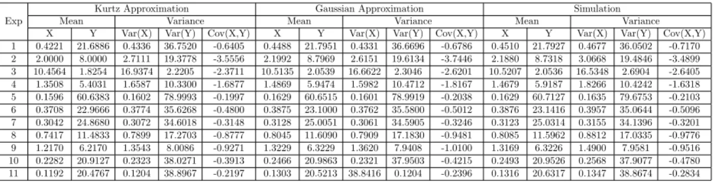
3.1
Comparison of simulation and approximation . . . 51
3.2
Comparison of simulation and approximation . . . 51
3.3
R
o(
T
) and
R
h(
T
) for HPKA1 . . . 72
3.4
R
o(
T
) and
R
h(
T
) for HPGA1 . . . 72
3.5
R
o(T
) and
R
h(T
) for HPKA2 . . . 76
LIST OF FIGURES
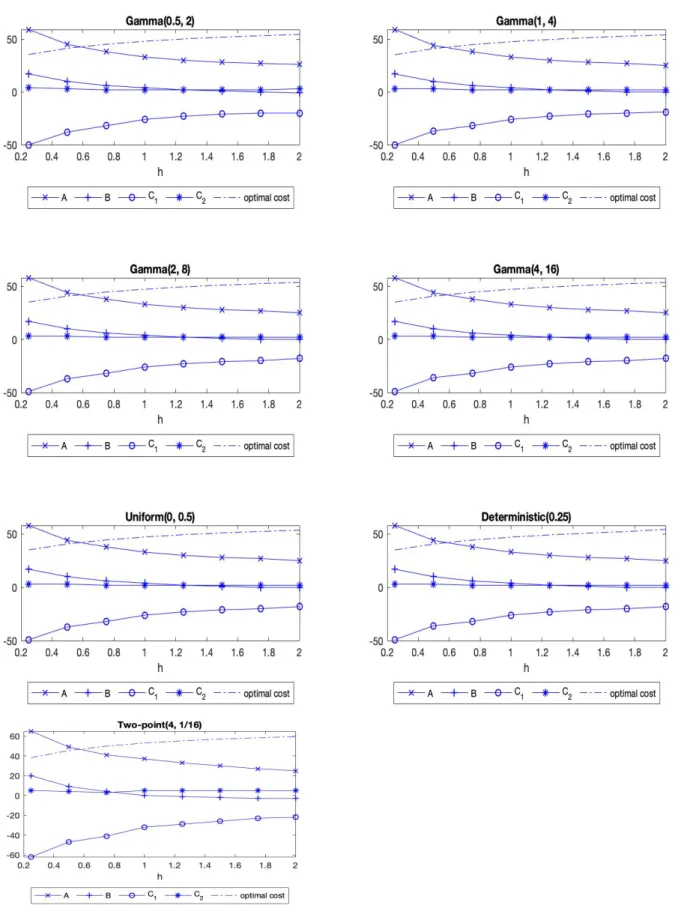
2.1
Optimal (
A, B, C
1, C
2) policies and optimal costs for different distributionswith mean equal to 0.25 as
h
varies for G+M case . . . 22
2.2
Optimal (
A, B, C
1, C
2) policies and optimal costs for different distributions
with mean equal to 0.25 as
µ
varies for G+M case . . . 23
2.3
Optimal (
A, B, C
1, C
2) policies and optimal costs for different distributionswith mean equal to 0.25 as
r
2varies for G+M case . . . 24
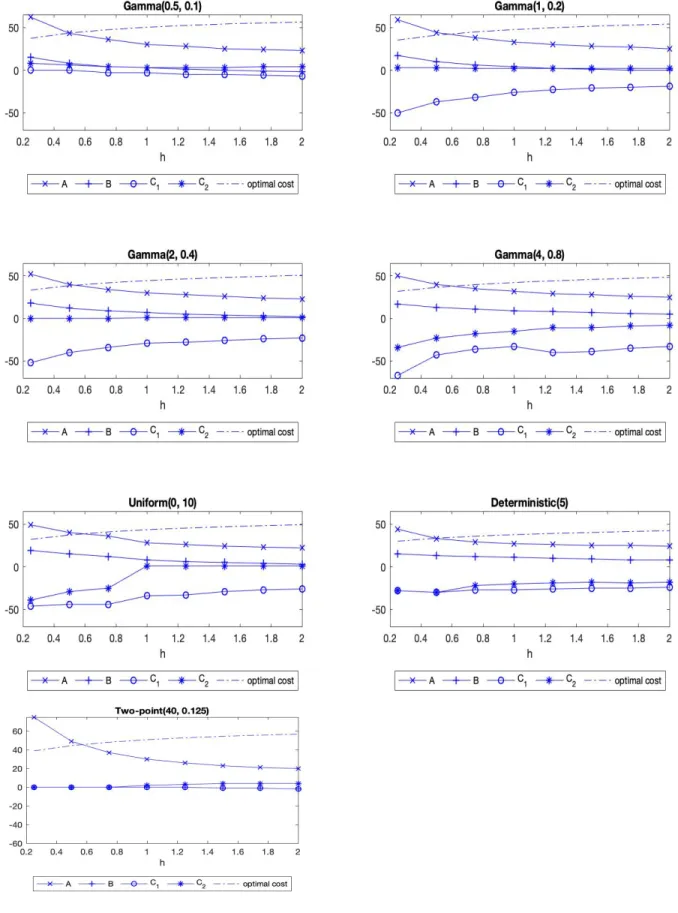
2.4
Optimal (
A, B, C
1, C
2) policies and optimal costs for different distributions
with mean equal to 5 as
h
varies for M+G case . . . 27
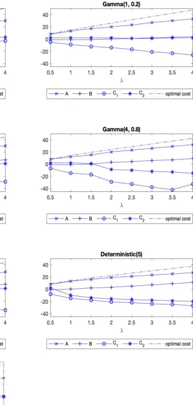
2.5
Optimal (
A, B, C
1, C
2) policies and optimal costs for different distributions
with mean equal to 5 as
λ
varies for M+G case . . . 28
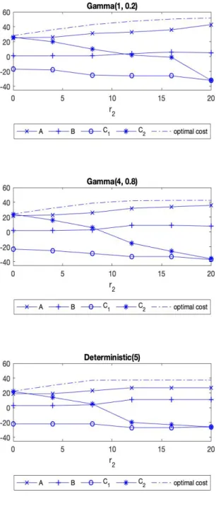
2.6
Optimal (
A, B, C
1, C
2) policies and optimal costs for different distributionswith mean equal to 5 as
r
2varies for M+G case . . . 29
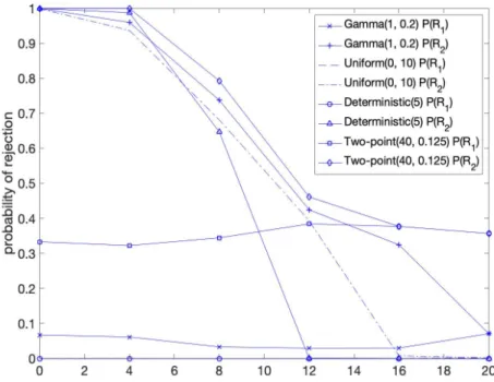
2.7
Probabilities of rejecting class 1 and class 2 demands as
r
2varies for M+G case . . . 30
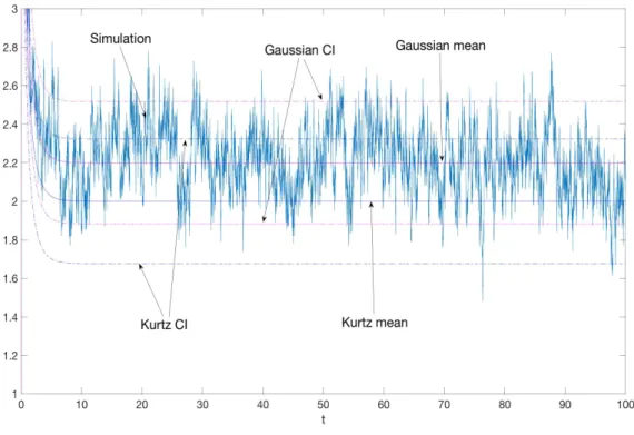
3.1
Kurtz’s approximation and the Gaussian Approximation approximation to
{
X
(
t
)
,
0
≤
t
≤
100}
. . . 53
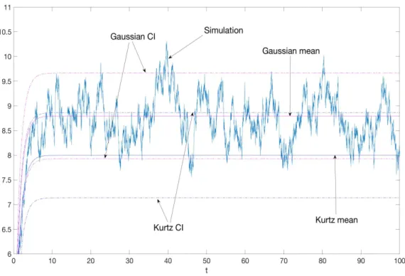
3.2
Kurtz’s approximation and the Gaussian Approximation approximation to
{
Y
(
t
)
,
0
≤
t
≤
100}
. . . 54
3.3
Kurtz’s approximation and the Gaussian approximation to
{
X
(
t
)
,
0
≤
t
≤
24}
. . . 56
3.4
Kurtz’s approximation and Gaussian approximation to
{
Y
(
t
)
,
0
≤
t
≤
24}
. . . 57
3.5
Optimal accpetance/rejection region . . . 59
3.6
x
(
t
),
y
(
t
) and
µ
∗(
t
) for Kurtz’s and Gaussian Approximations for first order
model . . . 66
3.7
x
(
t
),
y
(
t
) and
µ
∗(
t
) for Kurtz’s and the Gaussian Approximations at the
beginning of the day (
t
∈
[0
,
1]) for first order model . . . 67
3.8
x
(
t
),
y
(
t
) and
µ
∗(
t
) for Kurtz’s and Gaussian Approximations for constant
λ
(
t
) for second order model . . . 68
3.9
x
(
t
),
y
(
t
) and
µ
∗(
t
) for Kurtz’s and the Gaussian Approximations at the
beginning of the day (
t
∈
[0
,
1]) for second order model . . . 68
3.10 The optimal
x
(
t
),
y
(
t
) and
x
h(t
),
y
h(t
) for HPKA1 . . . 73
3.11 The optimal ¯
x
(
t
), ¯
y
(
t
) and ¯
x
h(
t
), ¯
y
h(
t
) for HPGA1 . . . 74
3.13 The optimal ¯
x
(
t
), ¯
y
(
t
) and ¯
x
h(
t
), ¯
y
h(
t
) for HPGA2 . . . 78
3.14 The optimal
x
(
t
),
y
(
t
) and
µ
∗(
t
) for Kurtz’s Approximation and the optimal
¯
x
(
t
), ¯
y
(
t
) and
µ
∗(
t
) for Gaussian Approximations for sine
λ
(
t
) for the first
order model . . . 82
3.15 The optimal
x
(
t
),
y
(
t
) and
µ
∗(
t
) for Kurtz’s Approximation and the optimal
¯
x
(
t
), ¯
y
(
t
) and
µ
∗(
t
) for Gaussian Approximations for sine
λ
(
t
) for the second
order model . . . 83
A.1 Optimal (
A, B, C
1, C
2) policies and optimal costs for different distributions
with mean equal to 0.25 as
h
varies for G+M case . . . 95
A.2 Optimal (
A, B, C
1, C
2) policies and optimal costs for different distributionswith mean equal to 0.25 as
µ
varies for G+M case . . . 96
B.1 Optimal (
A, B, C
1, C
2) policies and optimal costs for different distributions
with mean equal to 5 as
h
varies for M+G case . . . 100
B.2 Optimal (
A, B, C
1, C
2) policies and optimal costs for different distributionsCHAPTER 1
Introduction
The dissertation consists of two projects. We include the details in the next two chapters.
Chapter 2 considers a single-item inventory system with multiple demand classes. We introduce a
four-parameter policy, and use Markov Regenerative processes and Genetic Algorithm to study such
a system. Chapter 3 stuides a system of customers and taxis. We introduce a delayed matching
process between taxis and customers, and propose two methods to approximate the system. We
also study an optimal control problem and develop a heuristic policy for such a system.
the same mean can introduce significant errors. The numerical optimality is done using Genetic
Algorithm.
CHAPTER 2
USING GENETIC ALGORITHM AND MARKOV REGENERATIVE
PRO-CESSES
FOR
INVENTORY
SYSTEMS
WITH
MULTIPLE
DEMAND
CLASSES
2.1
Introduction
A single-item inventory system with multiple demand classes is frequently observed in real
world. For such a system, inventory rationing is an important tool to balance supply and demand.
[Ha, 1997] provides two examples in his paper. One is a multiechelon inventory system which is
characterized by emergency shortage shipments and regular shipments to satisfy demands. The
other is a commonality strategy employed by many manufacturers, where one common
compo-nent is used for mutiple endproducts, but one endpoint may have higher priority over the others.
[Deshpande et al., 2003] also give an example of an inventory rationing problem of US military.
Inventory systems with a single demand class have been studied extensively. When the
pro-duction orders are delivered immediately (no lead times), the optimal policies are of (
s, S
) type,
i.e., when the inventory level (inventory on hand
−
inventory on backorders) drops to or below
s
,
we place an order to bring the inventory level to
S
, see [Arrow et al., 1958], [Scarf, 1960]. With
lead times, if there is no restriction on the number of outstanding orders and no order crossing
is allowed, the optimal policy is still of (
s, S
) type, see [Ehrhardt, 1984], [Song et al., 2000]. In
this case, the optimal policy is based on inventory position (inventory level + on-order inventory).
We have to use two-dimensional processes to formulate the model. To avoid these problems, some
papers ([Browne and Zipkin, 1991], [Liu and Kulkarni, 2009], [Kulkarni and Yan, 2012], [Song and
Zipkin, 1996]) consider an inventory system with an (
r, Q
) policy, i.e., when the inventory level
drops to or below
r
, we place an order of size
Q
. Then one can obtain the optimal (
r, Q
) policy
which minimizes the long-run average cost.
one outstanding order at any time. For such a system, there are mainly two decisions that need to
be made. The first one is whether to satisfy an incoming demand or not. Demands from different
classes have different priorities which are usually characterized by class-specfic penalty costs and
backorder costs, etc. Thus it makes sense to reserve some items for future demands from higher
priority class by rejecting demands from the lower priority class. This rejection decision depends
on the inventory level and the status of the production. The second decision is when to place a
production order and what the order size should be. Intuitively, when the inventory level is high,
no production order should be placed, to avoid additional ordering and holding costs. When the
inventory is low, an order should be placed to reduce the rejection penalty and backorder costs.
The optimal order size is determined by current inventory level: we should order (or produce) more
if the inventory level is lower.
When demands arrives according to independent Poisson processes and the production lead
times are
iid
exponential and the order size
A
is fixed, we formulate the problem as a Markov
De-cision Process (MDP). We derive methods of computing the long-run average cost and numerically
obtain the optimal policy that minimizes the long-run average cost. Our numerical results show
that the optimal policy is of (
A, B, C
1, C
2) type. In addition, when
A
= 1, we prove the optimality
and the structural properities of the (1
, B, C
1, C
2) policy.
When either the demand interarrival times or the lead times are not exponential, the MDP
methodology cannot be used in a tractable way. Hence, in these cases we restrict our attention
to (
A, B, C
1, C
2) policies. We develop tractable methods to evaluate the performance of suchpoli-cies. We find that the optimal (
A, B, C
1, C
2) policies and the minimum long-run average costs arefairly insensitive to the arrival processes when the interarrival times of the demands follow Gamma,
uniform or deterministic distribution. Thus Poisson process can be used as an approximation to
general arrival process. However, the optimal (
A, B, C
1, C
2) policies and corresponding minimum
long-run average costs are quite sensitive to the lead time distributions. Therefore,
approximat-ing the general distribution of production lead times by exponential distribution can introduce
significant errors.
numerically show that the (
A, B, C
1, C
2) policy is optimal for
A >
1. Second, we consider cases
when the demand interarrival times and the production lead times are generally distributed. We
model the stochastic processes as Markov regenerative processes and develop tractable expressions
for the long-run average cost. Using these we compute the optimal (
A, B, C
1, C
2) policies using theGenetic Algorithm.
The remainder of this paper is organized as follows. First we provide a brief review of the related
literature and position our paper in the relevant context in Section 2.2. Section 2.3 describes the
(
A, B, C
1, C
2) policy. In Section 2.4, we analyze the case when then demands arrives according
to Poisson processes and the production lead times are exponential. In Section 2.5 and Section
2.6, we study the cases when the demand interarrival times or the production lead times are not
exponential. The paper concludes in Section 2.7 with an overall summary and a discussion of
possible extensions.
2.2
Literature Survey
Over the years many reseachers have studied production-inventory problems involving multiple
customer classes. [Ha, 1997] considers a single-item, make-to-stock production system with several
demand classes for the case of Possion demands and exponential production lead times. The system
produces one item at a time, demands that cannot be satisfied immediately are lost. He shows that
the optimal production policy is a base-stock policy, and the optimal inventory policy is a
stock-reservation policy, which is characterized by a sequence of monotone rationing levels corresponding
to different demand classes. When a demand of a certain class arrives, if the inventory level is
above the rationing level of that class, the demand is satisfied, otherwise the demand is lost. In the
numerical study, he shows that this rationing policy performs better than the first-come first-serve
policies that do not employ rationing. Later, [Ha, 2000] extends his analysis to the case of Erlang
distributed production lead times, where a variable
work storage level
is introduced to capture the
information regarding inventory level and staus of the outstanding order.
distributed. At any time, one can choose whether to produce type 1 or type 2 or to idle the machine.
They give a characterization of the switching curve that determines the production priorities using
sample path comparison for hedging point policies. Their results suggest that when both products
are backlogged, it is optimal to produce the item with higher backorder cost until its stock reaches
some predetermined level before switching to produce the item with lower backorder cost. This
level does not depend on the level of backlogs of the product with lower backorder cost.
[De V´
ericourt et al., 2001] also compute the optimal parameters and compare the performance
of the three allocation policies: FCFS, strict priority policy and multilevel rationing policy. Under a
strict priority policy, demands are satisfied (or backlogged) regardless of their classes, backorders are
cleared according to their priorities. Multilevel rationing policy is similar to the stock-reservation
policy in [Ha, 1997], which is characterized by a sequence of monotone critical levels. An arriving
demand of a certain class is satisfied with the stock if the inventory level is above the critical level
of that class, otherwise it is backlogged. Their numerical results show that the multilevel policy
always outperforms the other two policies.
[Deshpande et al., 2003] analyze a rationing policy for a single item system in a (
Q, r, K
)
envi-ronment for the inventory system with two demand classes with Poisson arrivals and deterministic
lead times. The inventory is replenished according to a (
Q, r
) policy where a production order of
size
Q
is placed whenever the inventory position drops to
r
. Demands for both classes are fulfilled
on a first-come-first-served (FCFS) basis, as long as the on-hand inventory is above the rationing
level
K
. Demands from the lower priority class (class 2) are backordered once the on-hand inventory
falls below
K
, but demands from higher priority class (class 1) are still satisfied as long as there is
on-hand inventory. Demands from class 1 are backordered only when on-hand inventory drops to
zero. Backorders are cleared according to a threshold clearing mechanism: first clear all backlogged
demands in an FCFS fashion that arrive before (
r
+
Q
−
K
)th demands arrives; then clear any
remaining class 1 backorders until either all class 1 backorders are filled or no on-hand inventory
remains, and continue to backlog class 2 demands arriving after (
r
+
Q
−
K
)th demands arrives.
Their numerical results show that the solution under this special threshold clearing mechanism
closely approximates that of the priority clearing policy.
[Kranenburg and van Houtum, 2007] present three accurate and efficient heruristic algorithms to
find the optimal critical values that minimize the cost at a given base stock level, for a lost sales
system with Poisson demands and arbitrary lead times. They test the accuracy in an extensive
computational experiment, and the results show that all the three heuristics produce an optimal
solution in all instances.
[Teunter and Haneveld, 2008] study inventory systems with two demand classes (critical and
non-critical), Poisson demands, fixed lead times and backorders. They analyze dynamic rationing
strategies where the number of items reserved for critical demand depends on the remaining time
until the next order arrives, and derive a set of formulae that determine the optimal rationing level
for any possible value of the remaining time. Their numerical examples illustrate that this dynamic
rationing strategy outperforms all static strategies with fixed rationing levels.
[Fadilo˘
glu and Bulut, 2010] extend the (
Q, r, K
) policy in [Deshpande et al., 2003] by defining
a modified on-hand inventory level which captures the information on the status of the outstanding
orders. Under this dynamic policy, demands of lower priority class are satisfied only if the modified
on-hand inventory is above some critical level
K
. Backorder clearing mechanism is also modified
accordingly: after clearing backorders from higher priority class (if any), the remainder of the order
(if any) is first used to increase the modified on-hand level up to
K
and then clear the backorders
of lower priority class.
[Ghosh et al., 2015] introduce a new class of two bin policy for the inventory system with two
demand classes, Poisson arrivals and fixed lead times. This policy assigns separate two bins of
inventory for the two demand classes: when the bin intended for the higher demand class is empty,
demand from the higher class can still be fulfilled with the inventory from the other bin. Backorders
are cleared according to the policy in [Deshpande et al., 2003]. Results of their numerical study
show that the two bin policy provides a much higher service level for the lower priority class demand
without increasing the cost too much and without affecting the service level for the higher priority
class. When a minimum fill rate requirement is imposed on the lower priority class demand, the
two bin policy outperforms the critical level rationing policy in most instances.
outstanding at any time. They show that the optimal order policy is characterized by a reorder
point and the optimal rationing policy is characterized by time-dependent rationing levels. They
then generalize the model to multiple outstanding orders using the Erlang distribution. They also
introduce a state-transformation approach to perform the structural analysis and show that both
the reorder point and rationing levels are state dependent. Finally they show the monotonicity
of the optimal reorder point and rationing levels for the outstanding orders. In their paper, they
assume that the order size is fixed and show the convexity of the value function. However, how to
choose the optimal order size is not dicussed. In our work, we allow backorders and show how to
choose the optimal order size. When the order size is 1, we are able to show the convexity of the
value function of the MDP and derive the structural properties of the optimal policy. When the
order size is greater than 1, the convexity doesn’t hold.
As we can see, all of these previous papers assume that demands arrive according to Poisson
processes, and most of the papers assume exponential or fixed lead times or fixed order size. In our
paper, we futher extend the analysis to the cases where the arrival processes and the production lead
times have more general distributions. In addition, to simplify our analysis, we use two assumptions
which are different from some of the above papers: first we suppose that no more than one order
is outstanding at any time point; second, when backorders are allowed, we backlog demands from
both classes. When an outstanding order arrives, we fill class 1 backorders before class 2 backorders.
We describe our model in more details in the next section.
2.3
(
A, B, C
1, C
2)Policy
demands of both classes, and the backlogging cost is
b
per backlogged item per unit time. When
an order arrives, we preferentially fill class 1 backorders before we fill class 2 backorders. Let
h
be
the holding cost per item per unit time in the inventory.
At any time, we may place an order of size
A
, a given fixed constant. The cost of an order is
K >
0, another fixed number. We pay for the order when it arrives. We assume that the order
arrives in its entirety after a random lead time, and the mean lead time is 1
/µ
.
In this paper, we consider a four-parameter (
A, B, C
1, C
2) policy which operates as follows:
under an (
A, B, C
1, C
2) policy, we reject the class
k
demands when the on-hand inventory level is
at or below
C
k(
k
= 1
,
2). When the inventory level is at or below
B
, we place an order of size
A
. Note that since class 2 is of lower priority, we have
C
2≥
C
1, which means that we reject class
2 demands before we reject class 1 demands. Also, we must have
C
1≤
0, since it does not make
sense to reject class 1 demands when there are items on hand. The paramter
A
is called the order
size, the parameter
B
is called the reorder point, and the parameters
C
kare called rationing levels
for class
k
.
We develop stochastic processes that enable us to compute the performance of a given
(
A, B, C
1, C
2) policy. We can then find the optimal parameters that will optimize the performance.
Let
I
(
t
) be the inventory level at time
t
. Note that the inventory level cannot be lower than
C
1. We can only place an order when
I
(
t
)
≤
B
, and if the outstanding order arrives before any
demands occur, the inventory immediately after the order arrives is less than or equal to
A
+
B
.
Thus, the state space of
{
I
(
t
)
, t
≥
0}
is given by
S
=
{
C
1, C
1+ 1
, ..., A
+
B
}
.
Note that there is an outstanding order at time
t
if
C
1≤
I
(
t
)
≤
B
and no outstanding order if
B
+ 1
≤
I
(
t
)
≤
A
+
B
.
In the following we shall first compute the limiting distribution of
{
I
(
t
)
, t
≥
0}
assuming it
exits. Let
p
i= lim
Once the limiting distribution is computed, the expected holding cost rate
H
, the expected
penalty cost rate for rejecting demands
R
, the expected procurement cost rate
P
, and the expected
backorder cost rate
BC
can be computed. The long run average cost rate
T C
is given by
T C
=
H
+
R
+
P
+
BC.
(2.2)
Note that computing the total expected discounted cost involves transient analysis of the
{
I
(
t
)
, t
≥
0}
process and is more involved. Hence we do not attempt it here. Also, the average cost
is a reasonable performance measure for comparing different policies and hence is sufficient for our
purpose.
We consider several special cases of the above system under (
A, B, C
1, C
2) policies
depend-ing upon the distributional and operational assumptions. We describe these models by usdepend-ing a
nomenclatue similar to queueing models as follows:
Demand interarrival distribution + lead time distribution.
The interarrival times can be exponential (M), or general (G). The lead time can be exponential
(M), or general (G). Successive lead times are i.i.d.. We consider the following three models: M+M,
M+G, G+M.
In case the interarrival times are general, we assume that the interarrival times of the combined
demands are i.i.d. with common cdf
G
and each arrival is of class
k
(
k
=1, 2) with probability ˆ
p
k(ˆ
p
1+ ˆ
p
2= 1).
2.4
M+M Model
function of the state of the system. To be precise, suppose the optimal ordering policy is described
by a critical number
B
such that it is optimal to accept an order when the inventory level is
B
or less. Since the inventory level decreases between accepted orders, and the order lead time is
exponential, this is equivalent to placing an order when the inventory level is
B
or less. We shall
follow this alternate set up since it simplifies the analysis.
It is clear that the state is described by a state variable
I
(
t
), where
I
(
t
)
∈
Z
=
{0
,
±1
,
±2
, ...
}
is the inventory level at time
t
. The state space is then given by
S
=
Z
.
The decision epochs are the demand arrival times and the order arrival times. When a demand
occurs in state
i
, we need to decide whether or not to satisfy it. When an order arrives, we need
to decide whether to accept or reject it.
Let
c
(
i
) =
hi,
i
≥
0
,
−
bi,
i <
0
.
We use uniformization to convert the continuous time MDP into a discrete time MDP. We scale the
time so that
λ
1+
λ
2+
µ
= 1. The analysis of the long-run average cost involves finding a constant
g
and a bias function
f
:
S
→
(−∞
,
∞) that satisfies the following optimal equation.
g+f(i) =c(i) +µmin{f(i), f(i+A) +K}+λ1min{f(i−1), f(i) +r1}+λ2min{f(i−1), f(i) +r2},
(2.3)
Suppose there is a solution to the above equation. Then a class
k
demand arrives in state
i
, it
is optimal to satisfy it if
f
(
i
) +
r
k≥
f
(
i
−
1)
,
(2.4)
and not satisfy it otherwise. Also, it is optimal to reject an order of size
A
if
f
(
i
+
A
) +
K > f
(
i
)
.
(2.5)
We first establish that there is a solution
g
and
f
to (2.3). We begin by stating a theorem from
[Weber and Stidham, 1987], which gives a set of conditions under which the limit of
γ
-discounted
policies yields the average cost optimal policy.
Theorem 1.
Let
v
γ(
x
)
be the minimum expected total discounted cost over the infinite horizon when
starting in state
x
and discounting factor
γ
. Suppose a general Markov decision process satisfies
the following conditions:
(a) There exists an
x
γsuch that
v
γ(x
γ)≤
v
γ(x
)
for all
x
.
(b) The state space
X
is countable.
(c) The set of actions
A
(
x
)
which is available in state
x
is a compact metric space.
(d) The probability
P
a(
x, y
), of transition to state
y
when action
a
is taken in state
x
, is
continuous in
a
∈
A
(
x
).
(e) The one-stage cost
c
a(
x
), of taking action
a
in state
x
, is non-negative and continuous in
a
∈
A
(
x
).
(f ) It is possible to go from any state
x
to any other state
y
, with finite expected cost.
(g) For each
x
there are only finitely many
y
for which
P
a(x, y
)
>
0
for some
a
∈
A
(
x
).
(h) If there is some policy which achieves a finite average cost, say
η
∗, then the number of states
in which the one-stage cost can be no more than
η
∗is finite.
Then
(i) The minimum long-run average cost exists, and is given by
g
= lim
γ→0γv
γ(
x
γ).
(ii)
v
γ(
x
)
−
v
γ(
x
γ)
converges to a limit
f
(
x
)
as
γ
tends to 0.
(iii)
f
(·)
satisfies
g
+
f
(
x
) = inf
a∈Ax{
c
a(x
) +
X
yP
a(x, y
)
f
(
y
)}
.
The main result is given in the following theorem.
Theorem 2.
The optimality (2.3) has a unique solution
(
g, f
).
Proof.
The state space is
S
=
Z
. We verify the conditions in Theorem 1 one by one.
(a) For our model, let
v
γ(
i
) be the minimum expected total discounted cost. It is obvious that
we can find an
i
0, such that
v
γ(
i
)
> M
0for all
|
i
|
> i
0.. Among states
{
i
:
i
=
±0
, ...,
±
i
0}, there is
a mimimum
m
=
v
γ(i
γ) andm
≤
v
γ(0). Sincev
γ(i
)
> M
0> v
γ(0)≥
m
for
i
=
|
i
0|
+ 1
,
|
i
0|
+ 2
, ...
,
m
=
v
γ(i
γ)≤
v
γ(i
) for all
i
.
(b) The condition holds since
i
= 0
,
±1
,
±2
, ...
.
(c) Let
U
(
i, s
) =
{
u
0(i
)
, u
1(i
)
, u
2(i
)}
be the set of actions which is available in state
i
, where
u
0(i
) = 0 if we reject an incoming order,
u
0(i
) = 1 if we accept an incoming order,
u
k(i
) = 0 if
an incoming demand of class
k
is satisfied, and
u
k(
i
) = 1 if an incoming demand of class
k
is not
satisfied (
k
= 1
,
2). Then
U
(
i
)
⊂ {0
,
1} × {0
,
1} × {0
,
1}, thus
U
(
i
) is a compact metric space.
(d) Since
U
(
i
) is a discrete set,
P
u(
i, j
) is continuous in
u
∈
U
(
i
).
(e) Same as (d).
(f) For any state
i
, we can increase
i
by accepting an order and decrease it by not satisfying
incoming demands. Thus it is possible to go from any state
i
to any other state
j
in a finite number
of steps. In each step, the expected cost is finite. Therefore, the total expected cost is finite.
(g) For each
i
, we can only go from it to finitely many states
j
in one step: for
j
can be
i, i
−
1
, i
+
A
. Only for such
j
’s
P
u(
i, j
)
>
0.
(h) Since
c
u(
i
)
≥
max{
b, h
}|
i
|, states in which the one-stage cost is no more than
η
∗should
satisfy
|
i
| ≤
maxη{∗b,h}. Therefore the number of states
i
is bounded by
max2η{∗b,h}, which is finite.
Thus
v
γ(
i
)
−
v
γ(0) converges to
f
(
i
) as
γ
→
0 and
v
r(0) converges to
g
. Furthermore,
g
and
f
satisfy (2.3).
Equation (2.3) can be solved by the value iteration method of [Tijms, 2003]. Next we will show
that if
f
is convex, there is a unique optimal (
A, B, C
1, C
2) policy that minimizes the long-run
average cost.
Theorem 3.
If
f
is convex in
i
, then
(
A, B, C
1, C
2)
is optimal when
B
= max{
i
:
f
(
i
+
A
)
−
f
(
i
)
≤ −
K
}
,
(2.6)
Proof.
Let
B
be as given in (2.6), then
f
(
B
+
A
+ 1)
−
f
(
B
+ 1)
≥ −
K
. Hence for
i > B
, since
f
is convex in
i
, we have
f
(
i
+
A
)
−
f
(
i
)
≥
f
(
B
+
A
+ 1)
−
f
(
B
+ 1)
>
−
K
Thus it is optimal to accept an order if
i > B
. For
i
≤
B
,
f
(
i
+
A
)
−
f
(
i
)
≤
f
(
B
+
A
)
−
f
(
B
)
≤ −
K,
hence it is optimal to reject an incoming order when
i
≤
B
.
Let
C
kbe as given in (2.7), then
f
(
C
k+ 1)
−
f
(
C
k)>
−
r
k. Hence convexity impliesf
(
i
)
−
f
(
i
−
1)
≥
f
(
C
k+ 1)
−
f
(
C
k)
≥ −
r
k, i > C
kThus it is optimal to satisfy the demand of class
k
if
i > C
k. Fori
≤
C
k.f
(
i
)
−
f
(
i
−
1)
≤
f
(
C
k)
−
f
(
C
k−
1)
≤ −
r
kHence it is optimal not to satisfy the demand when
i
≤
C
k.One can show that when
A
= 1,
f
is convex in
i
. The proof is given as follows.
Theorem 4.
When
A
= 1,
f
(·)
is convex.
Proof.
Let
v
n(i
) be the minimum expected total cost over
n
events when starting in state
i
. It can
be computed recursively using the following equation, starting with
v
0(i
) = 0,
∀
i
∈
S
.
vn+1(i) =c(i) +µmin{vn(i), vn(i+ 1) +K}+λ1min{vn(i−1), vn(i) +r1}+λ2min{vn(i−1), vn(i) +r2},
By Theorem 1, we know that
f
(
i
) = limn(
v
n(i
)
−
v
n(0)). We will prove the theorem by induction.Assume that
v
nis convex in
i
, i.e. for a given
n
≥
0, for all
i
∈
S
,
v
nsatisfies
Since
v
0(
i
) = 0,
∀
i
∈
S
, (2.8) holds for
n
= 0. Now suppose it holds for some
n
≥
0. Then we have
v
n+1(i
+ 1) +
v
n+1(i
−
1)
−
2
v
n+1(i
)
≥
µ
∆1
+
λ
1∆2+
λ
2∆3,
(2.9)
where
∆1
= min{
v
n(i
+ 1)
, v
n(i
+ 2) +
K
}
+ min{
v
n(i
−
1)
, v
n(i
) +
K
} −
2 min{
v
n(i
)
, v
n(i
+ 1) +
K
}
,
∆2
= min{
v
n(i
)
, v
n(i
+ 1) +
r
1}
+ min{
v
n(i
−
2)
, v
n(i
−
1) +
r
1} −
2 min{
v
n(i
−
1)
, v
n(i
) +
r
1}
,
∆
3= min{
v
n(
i
)
, v
n(
i
+ 1) +
r
2}
+ min{
v
n(
i
−
2)
, v
n(
i
−
1) +
r
2} −
2 min{
v
n(
i
−
1)
, v
n(
i
) +
r
2}
.
We will show that ∆1
≥
0, ∆2
≥
0, and ∆3
≥
0, then RHS of (2.9)≥
0 and hence (2.8) also holds
for
n
+ 1.
We first prove that ∆1
≥
0. If
min{
v
n(
i
+ 1)
, v
n(
i
+ 2) +
K
}
=
v
n(
i
+ 2) +
K,
the convexity of
v
nimplies that
min{
v
n(
i
−
1)
, v
n(
i
) +
K
}
=
v
n(
i
) +
K.
Thus,
∆1
≥
v
n(i
+ 2) +
K
+
v
n(i
) +
K
−
2(
v
n(i
+ 1) +
K
) =
v
n(i
+ 2) +
v
n(i
)
−
2
v
n(i
+ 1)
≥
0
by induction hypothesis.
If
min{
v
n(i
+ 1)
, v
n(i
+ 2) +
K
}
=
v
n(i
+ 1)
,
min{
v
n(i
−
1)
, v
n(i
) +
K
}
=
v
n(i
−
1)
,
then
∆1
≥
v
n(i
+ 1) +
v
n(i
−
1)
−
2
v
n(i
)
≥
0
.
If
min{
v
n(
i
+ 1)
, v
n(
i
+ 2) +
K
}
=
v
n(
i
+ 1)
,
min{
v
n(
i
−
1)
, v
n(
i
) +
K
}
=
v
n(
i
) +
K,
then
∆
1≥
v
n(
i
+ 1) +
v
n(
i
) +
K
−
(
v
n(
i
) +
v
n(
i
+ 1) +
K
) = 0
.
Therefore, ∆
1≥
0.
We next prove that ∆
2≥
0.
If
min{
v
n(i
)
, v
n(i
+ 1) +
r
1}
=
v
n(i
+ 1) +
r
1,
the convexity of
v
nimplies that
Thus,
∆
2≥
v
n(
i
+ 1) +
r
1+
v
n(
i
−
1) +
r
1−
2(
v
n(
i
) +
r
1) =
v
n(
i
+ 1) +
v
n(
i
−
1)
−
2
v
n(
i
)
≥
0
by induction hypothesis.
If
min{
v
n(i
)
, v
n(i
+ 1) +
r
1}
=
v
n(i
)
,
min{
v
n(i
−
2)
, v
n(i
−
1) +
r
1}
=
v
n(i
−
2)
,
then
∆2
≥
v
n(i
) +
v
n(i
−
2)
−
2
v
n(i
−
1)
≥
0
.
If
min{
v
n(i
)
, v
n(i
+ 1) +
r
1}
=
v
n(i
)
,
min{
v
n(i
−
2)
, v
n(i
−
1) +
r
1}
=
v
n(i
−
1) +
r
1,
then
∆2
≥
v
n(i
) +
v
n(i
−
1) +
r
1−
(
v
n(i
−
1) +
v
n(i
) +
r
1) = 0.
Hence, ∆
2≥
0. Similarly, one can show that ∆
3≥
0.
For
A >
1, the function
f
(·) is not convex, but our numerical study shows that the optimal
policy is still of the (
A, B, C
1, C
2) type, whereB, C
1, C
2are as given in (2.6) and (2.7)
Under this policy,
{
I
(
t
)
, t
≥
0}
is a CTMC. The set of recurrent states is given by
{
i
:
C
1≤
i
≤
A
+
B
}.
The rest of the states in
S
are transient. The positive transition rates are given by
q
C1,C1+A=
µ,
i
=
C
1,
q
i,i+A=
µ, q
i,i−1=
λ
1+
λ
2I
(
i > C
2),
C
1+ 1
≤
i
≤
B,
q
i,i−1=
λ
1+
λ
2I
(
i > C
2)
,
B
+ 1
≤
i
≤
A
+
B.
(2.10)
The expected holding cost rate
H
, the expected penalty cost rate for rejecting demands
R
, the
expected procurement cost rate
P
, and the expected backorder cost rate
BC
for the CTMC are
given by
H
=
h
A+B
X
i=1
ip
i,
(2.11)
R
=
λ
1r
1p
C1+
λ
2r
2 C2X
i=C1
p
i,
(2.12)
P
=
µ
(
K
+
cA
)
BX
i=C1
p
i,
(2.13)
BC
=
b
0
X
i=C1
Note that the cost of an order of size
A
is now modeled as
K
+
cA
in (2.13). This will allow us to
find an optimal
A
.
In order to find the optimal
A
, one can compute the optimal (
A, B, C
1, C
2) policy for each fixedA
, and find the value
A
which minimizes the long-run average cost. One can compute the long-run
average cost of an (
A, B, C
1, C
2) policy in (2.2), and then find the optimal (A, B, C
1, C
2) policy.The optimization has to be done numerically.
The numerical study of the M+M model is included in next sections, since the it can be
considered as a special case of the G+M and the M+G models.
2.5
G+M Model
In this section, we assume that the interarrival times of demands are iid with general distribution
F
(·) and mean
τ
. With probability ˆ
p
1, the arriving demand is of class 1; with probability ˆp
2= 1−
p
ˆ
1,it is of class 2. The production lead times are iid
exp
(
µ
). The optimal policy in this case is
intractable. Hence we restrict our attention to (
A, B, C
1, C
2) policies. The next theorem gives theprobabilistic structure of the
{
I
(
t
)
, t
≥
0}
process. (See [Kulkarni, 2009] for relevant definitions.)
Theorem 5.
{
I
(
t
)
, t
≥
0}
is a Markov regenerative process (MRGP) with state space
S
=
{
C
1, C
1+
1
, ..., A
+
B
}.
Proof.
Suppose the process starts in the initial state
I
0at time
t
= 0. Consider an increasing
sequence of times
{
S
n, n
≥
0}
defined as follows. Let
S
0= 0, and
S
n= the time when
n
-th demand arrives for
n
≥
1
.
Next we study the stationary distribution of
{
I
(
t
)
, t
≥
0}. We need the following to compute
this distribution.
G
ij=
P
(
I
n+1=
j
|
I
n=
i
)
,
(2.15)
τ
i=
E
(
S
1|
I
(0) =
i
) =
τ,
(2.16)
τ
ij=
E
(time spent by the MRGP in state
j
during [0
, S
1)|
I
(0) =
i
)
.
(2.17)
The expressions for
G
ijand
τ
ijare given in Appendix A.1. The limiting distribution of (2.1)
is then given by the following theorem.
Theorem 6.
Let
π
be the solution to
π
=
πG
and define
p
0k=
π
kτ
kP
A+Bi=C1
π
iτ
i=
π
kP
A+Bi=C1
π
i,
C
1≤
k
≤
A
+
B.
(2.18)
Then
{
I
(
t
)
, t
≥
0}
has a limiting distribution
[
p
i]i∈Swhich is given by
p
j=
A+BX
k=C1
p
0kτ
kjτ
k=
1
τ
A+B
X
k=C1
p
0kτ
kj,
C
1≤
j
≤
A
+
B.
(2.19)
Proof.
It is easy to see that the SMP generated by the MRS
{(
I
n, S
n), n
≥
0}
(see [Kulkarni, 2009])
is irreducible, positive recurrent and aperiodic, and its stationary distribution is given by (2.18).
Hence the result follows from the theory of MRGPs (see [Kulkarni, 2009]).
The expected holding cost rate
H
, the expected procurement cost rate
P
, and the expected
backorder cost rate
BC
are given by (2.11), (2.13), (2.14) respectively. For the G+M model, the
expected penalty cost rate for rejecting demands
R
is given by
R
= (ˆ
p
1r
1p
0C1+ ˆ
p
2r
2 C2X
i=C1
p
0i)
/τ.
(2.20)
Note that we need to use
p
0iin (2.20) instead of
p
ias in (2.12) in the CTMC case.
From Theorem 6 and the expressions for
G
ijand
τ
ij, we see that the limiting distribution
depends on the interarrival time distribution only via
τ
, ˜
F
(
µ
) =
R
∞0
e
−µt
dF
(
t
) and ˜
F
0(
µ
) =
−
R
∞0