LEARNING METHODS IN REPRODUCING KERNEL HILBERT SPACE BASED ON HIGH-DIMENSIONAL FEATURES
Hojin Yang
A dissertation submitted to the faculty at the University of North Carolina at Chapel Hill in partial fulfillment of the requirements for the degree of Doctor of Philosophy in the Department
of Biostatistics in the Gillings School of Global Public Health.
Chapel Hill 2016
Approved by: Joseph G. Ibrahim Hongtu Zhu John H. Gilmore Yun Li
c 2016 Hojin Yang
ABSTRACT
Hojin Yang: Learning Methods in Reproducing Kernel Hilbert Space Based on High-dimensional Features
(Under the direction of Joseph G. Ibrahim and Hongtu Zhu)
The first topic focuses on the dimension reduction method via the regularization. We propose the selection for principle components via LASSO. This method assumes that some unknown latent variables are related to the response under the highly correlate covariates structure. L1
regularization plays a key role in adaptively finding a few liner combinations in contrast to the persistent idea that is to employ a few leading principal components. The consistency of regression coefficients and selected model are asymptotically proved and numerical performances are shown to support our suggestion. The proposed method is applied to analyze microarray data and cancer data.
ACKNOWLEDGMENTS
First and foremost, I would like to thank my principal academic advisor Professor Joseph G. Ibrahim. I am grateful to him for his unwavering support for my academic activities. Apart from that, I am privileged to have had the opportunity to be acquainted with such as wonderful person. I would like to thank Professor Hongtu Zhu for his insightful comments about my research, for his painstaking efforts in improving the quality of my writing and for serving as my advisor. I thank Professor John H. Gilmore for his encouragement and advice and also for serving in my orals committee. I thank Professor Yun Li for serving in my orals committee. I thank Professor Eric Bair for his consistent advice and serving in my orals committee.
I am thankful to the entire faculty and the staff members of the department, for their efforts at resolving any problems I faced, and for providing a wonderful academic environment. I would like to thank Statisticians Allison Deal and Dominic Moore, my supervisors at Lineberger Comprehensive Cancer Center for their wonderful guidance and constant support.
TABLE OF CONTENTS
LIST OF TABLES . . . viii
LIST OF FIGURES . . . x
CHAPTER 1: INTRODUCTION AND LITERATURE REVIEW . . . 1
1.1 Introduction . . . 1
1.2 Principal Component Analysis . . . 2
1.2.1 Introduction for Principal Components . . . 2
1.2.2 Unsupervised vs Supervised Learning . . . 3
1.2.3 Limiting Spectral and Spike Model . . . 5
1.2.4 Sparse Principal Components . . . 6
1.3 Variable Selection . . . 7
1.3.1 Classical Regularization . . . 7
1.3.2 Modern Regularization . . . 8
1.3.3 Sure Independent Screening . . . 13
1.3.4 Two Stage Model . . . 15
1.4 Dimension Reduction . . . 15
1.4.1 Parametric Dimension Reduction . . . 15
1.4.2 Nonparametric Dimension Reduction . . . 18
1.4.3 Semiparametric Dimension Reduction . . . 19
1.5 Kernel Methods in Machine Learning . . . 20
1.5.2 Reviewing Methodologies in Machine Learning
on RKHS . . . 22
1.5.3 Statistics in Reproducing Kernel Hilbert Space . . . 23
CHAPTER 2: PRINCIPAL COMPONENTS SELECTION VIA LASSO . . . 26
2.1 Introduction . . . 26
2.2 Description . . . 28
2.2.1 Regression Method . . . 28
2.2.2 Motivation . . . 31
2.2.3 Choice Principle Components by LASSO in Regression . . . 34
2.2.4 Choice Principle Components by LASSO in Survival Analysis . . . 36
2.2.5 Tuning Parameter Selection . . . 39
2.2.6 Relation with the Eigenarray Space . . . 42
2.3 Simulation Studies . . . 42
2.3.1 Simulation 1: Single PC Cases . . . 42
2.3.2 Simulation 2: Multiple PC Cases . . . 47
2.4 Real Data Analysis . . . 49
2.5 Asymptotic Analysis . . . 54
2.6 Conclusion . . . 59
CHAPTER 3: MPM: MULTIPLE PROJECTION MODEL . . . 60
3.1 Introduction . . . 60
3.2 Description . . . 62
3.2.1 Model Setup . . . 62
3.2.2 Sure independent Screening via Positive Definite Kernel . . . 63
3.3 Simulation Studies . . . 69
3.3.1 Simulation 1: Prediction in Regression Problem . . . 69
3.3.2 Simulation 2: Prediction in Classification Problem . . . 74
3.3.3 Simulation 3: Prediction in Functional Curve Problem . . . 75
3.4 Real Data Analysis . . . 76
3.5 Conclusion . . . 79
CHAPTER 4: SILFM: SINGLE INDEX LATENT FACTOR MODEL BASED ON HIGH-DIMENSIONAL FEATURES . . . 83
4.1 Introduction . . . 83
4.2 SILFM: Single Index Latent Factor Model . . . 87
4.2.1 Model Setup . . . 87
4.2.2 Estimation Procedure . . . 88
4.3 Simulation Studies . . . 92
4.3.1 Simulation 1: Continuous Response (I) . . . 93
4.3.2 Simulation 2: Continuous Response (II) . . . 94
4.3.3 Simulation 3: Binary Response on Random Design . . . 97
4.4 Real Data Analysis . . . 99
4.5 Asymptotic Analysis . . . 103
4.6 Conclusion . . . 108
CHAPTER 5: DISCUSSION . . . 109
APPENDIX A: TECHNICAL DETAILS FOR CHAPTER 2 . . . 110
APPENDIX B: TECHNICAL DETAILS FOR CHAPTER 4 . . . 124
LIST OF TABLES
2.1 Model consistency in example 1. . . 45
2.2 Goodness of fit in example 1. . . 45
2.3 Model consistency in example 2. . . 48
2.4 Goodness of fit in example 2. . . 48
2.5 Description of data sets and results (n: number of data points, p: number of data dimensions, E: number of total events, ˆγmin: minimum penalty in Figure 2.2,ˆγ∗: criterion on 2.23 and PCs: number of selected PCs). . . 54
3.1 Model consistency in regression. . . 71
3.2 Sum of prediction error in regression. . . 71
3.3 Model consistency in classification. . . 72
3.4 Average of test error in classification. . . 72
3.5 Model consistency in functional curve. . . 73
3.6 Average of prediction error in functional curve. . . 73
3.7 Sum of prediction error in hippocampal surfaces data. . . 78
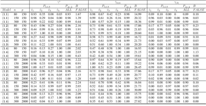
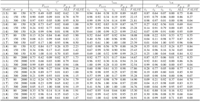
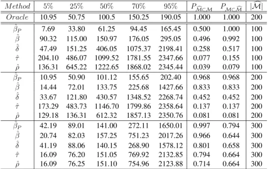
4.1 Performance of SIS methods in simulation 1: HSIC-SIS: screening with HSIC, DC-SIS: screening with correlation distance, SIS: screening with Pearson correlation, KD-SIS: screening with Kendall correlation, SP-SIS: screening with Spearman correlation,Ptp: true positive rate,PA: screening accuracy, Ptn: true negative rate, and Pf p: the false positive rate. . . 95
4.2 Average of prediction errors in simulation 1: Each column indicates the number of |M|c used for the prediction model. Each row presents a learning method. . . 95
4.4 Average of test error in simulation 3: SILFM: Projection by SILFM, KPCA: Projection by kernel PCs, PCA:
Projection by PCs SPCA: Projection by sparse PCs. . . 100 4.5 Sum of prediction errors in hippocampal surfaces data. . . 101 4.6 Prediction for behavior score in hippocampal surfaces
data:Yˆnumberis the prediction value, where the subscript number is the reduced feature dimension. Sums of prediction errors for Yˆ1000, Yˆ700 andYˆ500 were 117.3, 118.07and
118.01for 180 test observations. Correlation thresholding values were 0.3, 0.5 and 0.7. Estimated smoothing
LIST OF FIGURES
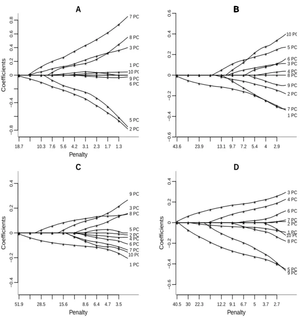
2.1 LASSO path for microarray datasets : (A) lung cancer data, (B) breast cancer data, (C) acute myeloid leukemia
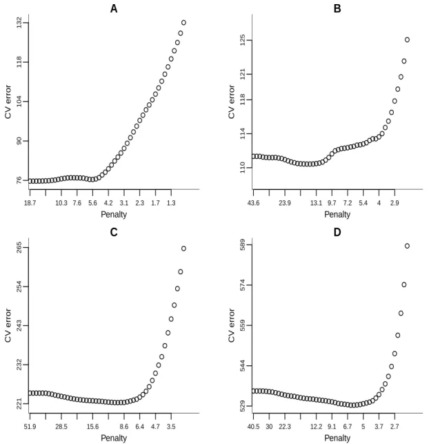
data and (D) DLBCL data. . . 50 2.2 Cross validation error for microarray datasets : (A)
lung cancer data, (B) breast cancer data, (C) acute myeloid
leukemia data and (D) DLBCL data. . . 51 2.3 Survival probability for microarray datasets : (A) lung
cancer data, (B) breast cancer data, (C) acute myeloid
leukemia data and (D) DLBCL data. . . 53
3.1 Images of correlation matrix : (A) left vs right, (B) reorder for both, (C) thresholding at 0.5 (D) thresholding
at 0.7. . . 81 3.2 Smoothing plots: (1) 30000, (2) 1000, (3) MMP at
1000. . . 81 3.3 Contour plots : (A) MMP, (B) KREG, (C) KPCA, (D)
KSPCA. . . 82 3.4 Smoothing plots : (A) MMP, (B) KREG, (C) KPCA,
(D) KSPCA. . . 82
4.1 Results from simulated data sets: the top row includes a selected covariate imagexi, an informative covariate image x˜i, a selected key feature zi versus a selected feature ofx˜i; the second row includes the scatter plotyi and the selected feature ofziand the average prediction error plots for SILFM1 (red) and SILFM2 (blue) and other competing methods (KRR (orange), SVM (skyblue), LASSO (green) SCAD (darkgreen), PLS (pink), SPLS (hotpink), PCA (black), SPCA (gray), and SSDR (purple))
in two simulation scenarios in subsection 3. . . 85 4.2 Path diagram of SILFM estimation procedure. . . 88 4.3 Averages of true positive rate for five different screening
4.4 Averages of prediction errors for 11 different predictive methods in simulation 2: all panels A (σy = 0.2, σx = 0.2), B (σy = 2, σx = 0.2), C (σy = 0.2, σx = 1), and D (σy = 2,σx = 1) report the results based on the
different levels ofσy andσx. . . 97 4.5 Correlation matrix for the top 1,000 features selected
from the left and right hippocampi. (A) left vs right, (B) reorder for both, (C) thresholding at 0.5 (D) thresholding
CHAPTER 1: INTRODUCTION AND LITERATURE REVIEW
1.1 Introduction
Accompanying the development of sciences and technologies, recent scientific data has charac -teristics of increasing in both complexity and size. One tendency of such complexity is the massive amount of available covariates called the ultrahigh dimensionality, which makes it hard the relationship between a response variables and the collection of the covariates. There are also challenges of noise accumulation, computational expediency, statistical accuracy and algorithmic stability due to such complexity. These challenges may need new statistical modeling techniques. Aims of this paper is to propose several dimension reduction methods via variable selection approaches and to improve the prediction performance by utilizing them in analyzing the ultrahigh dimensional data sets in numerous fields of science and engineering. The main subjective of this thesis is to concentrate on some specific aspects of dimension reduction, variable selection, and machine learning techniques.
response. While traditionally, the conditional mean in regression was described as the linear function, we assume that the conditional mean in the modeling is described as an arbitrary relationship where it may include both the linear and the non-linear relationship.
We will devise the methodology based on two stage model to address the ultrahigh dimensiona -lity. Our two stage model is divided by the dimension reduction stage and the estimating stage for the conditional mean. To reduce the problem of the large number of covariates, mainly two different approaches are available in statistical literature. Variable selection is the first approach where it is believed that only a few covariates, among all the available covariates, truly are relevant to the response, others are irrelevant and have no real explanatory effect. Various regularization and independent screening methods have been developed for a recent couple of decades to deal with ultra high dimensional data and these are clearly the representative methods in this area. It is the goal of variable selection to identify a few significant covariates. Dimension reduction is the second approach where it is believed that only a few linear combinations of the many covariates relates to the response. In contrast to the variable selection approach, all covariates could have explanatory effect, but the effect is only represented in a few linear combinations. To identify a few linear combinations from all covariates is the goal of dimension reduction. To estimate an unknown function within an arbitrary relationship, we employ the positive definite kernel based on theory of reproducing kernel Hilbert space. We will incorporate specific aspects of dimension reduction, variable selection, and machine learning techniques in favor of our circumstance in this paper.
1.2 Principal Component Analysis
1.2.1 Introduction for Principal Components
Principal component analysis (PCA) is one of the oldest and best popular methods for reducing dimensionality in multivariate problems. Let X1, X2, . . . , Xn be the vectors inRp. Let λ1 ≥ λ2 ≥ . . . ,≥ λp and θ1, θ2, . . . , θp be the eigenvalues and corresponding eigenvectors of Σ =
transformed variables,{θ10X, θ20X, . . . , θ0pX}. θjis called thej-th principal component direction. The sample version of principal components are{θˆ10X,θˆ20X, . . . ,θˆp0X}whereθˆ1 ≥θˆ2 ≥ · · · ≥θˆp andθˆ1,θˆ2, . . . ,θˆp are the eigenvalues and eigenvectors of the ordinal sample covariance matrix
ˆ Σ.
Adcock (1878) wrote the first page of history on principal components, finding the the most probable straight line or hyperplane determined bypdimensional coordinates of npoints. Pearson (1901) and Hotelling (1933) attempted to explain and analyze the complex statistical variables into principal components. Theoretically, Anderson (1963) derived the consistency of the principal components and the asymptotic distribution for fixedp.
There have been several reasons for why such reduction has been practical in statistical literature for a long time. In terms of traditional point of view, mitigating the effect of collinearity in regression problem and recovering signal structure in denoising process may be included as reasons. Since principal component analysis may be the best linear approximation capturing the maximum variability in covariates, it has been widely used in real data world.
1.2.2 Unsupervised vs Supervised Learning
Principle components have also been utilized to reduce dimensionality in the regression problem. Let Y be the response and suppose that our goal is to reduce the dimensionality of X before fitting a regression with the response Y for handling collinearity, providing low dimensional structure or constructing predictable and interpretable model.
particularly placed an emphasis on not doing the practice where reducible variables are selected by figuring out the relationship between the individual covariate and the response. Their belief may be in the spirit of the idea of the sufficiency. Consider the concept of the sufficiency
X|(T(X), Y) ∼X|T(X)
whereT is statistics. In other words, the reduction should be done, not depending on the response
Y but containing the same information for the covariatesX.
Cox (1968) however suggested entirely opposed thought in his article. He believed that there is no logical reason why the response should not be closely related to the least important principal component. He mentioned that If the covariatesXand the responseY have a joint distribution or there is an omitted variableZ which can be an external variable or an internal variable obtained by decomposing the linear combination derived from principal components, employing a few leading principal components is not appropriate. Hotelling (1957) attempted to explain this issue in factor model frame and Hawkins and Fatti (1984) explored the data representation through using minor principal components. Their belief may be in the spirit of the idea of the latent variable. Consider the regression model with the latent variable
Y =f(Z) +y, X =g(Z) +x
wheref andg are arbitrary functions. Consequently, the final goal of the dimension reduction can be the problem to estimate an omitted variableZ. The dimension reduction methodologies involving with the response Y is an appropriate approach since the response Y contains the information for Z. Partial least square estimator introduced by Helland (1988) and supervised principal components proposed by Bair et al. (2006) are representative methodologies utilizing the information for the responseY to reduce the dimensionality of the covariates.
principal components in regression model may be a simple and tricky problem. Jolliffe (2005) commented that the choice of principal components for the regression problem remains an open question.
1.2.3 Limiting Spectral and Spike Model
Principal components obtained by the reduction of dimensionality are vectors withpvariables in n observation. Contemporary data sets have much larger p thann, there arises the concern for the accuracy of principal components since Johnstone and Lu (2009) proved inconsistency of principal components aspandngoes to infinity while Anderson (1963) showed the consistency of them for fixed p. In other words, Johnstone’s condition that p/n → γ ∈ [0,∞) is more flexible than Anderson’s condition p/n → 0 in high dimensional data sets. Similar assertion happens to sample eigenvalues. SupposeX1, X2, . . . , Xnare observations from Gaussian model where mean zero and the covariance matrix is the identity matrix. Bai (1999) showed in his review paper that when the population covariance is the identity, the smallest and the largest eigenvalues of sample covariance matrix converge almost surely to (1−√γ)2 and(1 +√γ)2,
respectively. Under the circumstancep/n→γ, if0< γ < 1, then eigenvalues converge almost surely to near 1. There may be no great change but if γ ≥ 1, there may be a great change between the sample covariance matrix and the population covariance matrix in high dimensional data sets. Johnstone (2001b) derived the asymptotic distribution for the largest eigenvalue under this circumstance.
Assume thatX1, X2, . . . , Xn are observations from Gaussian model with mean zero and the covariance
Σ =diag(λ1, λ2, . . . , λM,1, . . . ,1)
recently introduced. Baik and Silverstein (2006) provedλˆj → (1 + √
γ)2 whenλj ≤ 1 + √
γ
and Bai et al. (2004) derived the asymptotic distribution of sample eigenvalue λˆj for the same circumstance. Paul (2007) showed the asymptotic distribution of sample eigenvalues for λj > 1 +√γ.
There are two importance in this subsection. The first message is that the result from the asymptotic spectral behavior, we may have an insight why principal components may not be a good tool in a high dimensional setting. The significant conditionp/n → γ ∈ [0,∞)showed by Johnstone and Lu (2009) is closely related to the asymptotic spectral behavior for the sample covariance. The second message is that phase transition phenomenon may be happened in a high dimensional data sets. This means when the ratioγ is larger than zero, the eigenvalues and sample covariance matrix are no longer reliable even ifΣ =I. Hence, spiked covariance model is a realistic structure in a high dimensional setting by magnifying the scale of eigenvalues or being comparable toγ.
1.2.4 Sparse Principal Components
Donoho (1993) and Johnstone (2003) introduced weak-lqspacewlq(C)space whereCandq are positive constants. Suppose that the coordinates of a vectorθ∈Rp are|v|
(1),|v|(2), . . . ,|v|(p)
where|v|(k)denotes thek-th largest element in absolute value. Then,wlq(C)space is defined as
θ∈wlq(C)⇔ |v|(k) ≤Ck−1/q, k= 1,2, . . . , p.
wlq(C)space is more general space thanLq(C)space since
θ ∈Rp∩Lq(C)⇒ p
X
i=1
|vi|q ≤Cq ⇒θ ∈wlq(C).
for some positive constantsqandC,
θ(n)∈wlq(C) asp→ ∞andn → ∞
where this condition is called a uniform sparsity condition. Then, they proposed an estimator for
k-th principal component
ˆ
θkIˆ=X j∈Iˆ
ˆ
θ∗jkej
whereθˆ∗jk = ˆθjkI{|θˆkj| ≥ δ} is given by hard thresholding, Iˆis the set of indices 1 ≤ j ≤ p
corresponding to the largest M variances (ˆσ2j = V ard(vij)) and θˆjk is k-th component of j-th
principal component. This thresholded estimator θˆIˆ is called sparse principal component and Johnstone and Lu (2009) showed its consistency under the uniform sparsity condition.
There are several different types of sparse principal components for the effort to obtain interpretable and predictable principal components. Zou et al. (2006) and Witten and Tibshirani (2008) suggested variant sparse principal components viaL1 regularization forθ. Those sparse
principal components have an similar objective function and constraints as the following
( ˆα,θˆ) = min α,θ
n
X
i=1
(Xi−αθ0Xi)2+µ p
X
j=1
|θj|
subject toα0α= 1.
1.3 Variable Selection
1.3.1 Classical Regularization
Suppose that we have (X1, y1),(X2, y2), . . . ,(Xn, yn) from the population (X, y) where it is assumed that the conditional expectation of Y given X is a linear function, β0X with
β = (β1, β2, . . . , βp)0. Goals of variable selection is to identify all significant variables whose coefficients are not zero and to estimate effective coefficients. It is one of important topics on not only parametric modeling but also nonparametric modeling. Akaike (1998) introduced AIC that minimizes Kullback-Leibler (KL) distance between the selected model and the true model for achieving aims. He showed that the asymptotic expansion of the estimated KL distance is given by
−ln( ˆβ) +λ
p
X
j=1
I( ˆβj 6= 0)
where ln is the log-likelihood function and λ = 1. Schwarz et al. (1978) devised BIC for
λ = logn. It is known that BIC with the larger observations provides a better result for estimating the dimension of true model than AIC. For the normal log-likelihood case, ln( ˆβ) becomesRSSd/σ2 whereRSSdis the residual sum of squares with the best dsubset. Mallows (1973) proposedCp =RSSd/s2+ 2d−nstatistics wheres2 is the variance estimator of the full model. Cross-validation proposed by Allen (1974) and generalized cross-validation introduced by Wahba and Wold (1975) also play a similar role in variable selection. All statistics mentioned here could be explained as the approach of penalized log-likelihood framework withL0 norm.
Li (1987) and Shao (1997) showed that those statistics are asymptotically equivalent for varying
λin the linear model.
1.3.2 Modern Regularization
Traditionally,L0regularization introduced in the previous subsection has been employed for
may be two difficulties. One difficulty mentioned by Fan and Li (2001) is that the existence of the most extreme value among coefficients makes the lack of stability and stochastic errors inherited in there procedure are ignored. Another difficulty is that computation is infeasible in a high-dimensional setting. Other regularization techniques have been developed for the last fifteen years to cope with difficulties in high dimensionality. Such regularization techniques can be generalized as
ln(β)− p
X
j=1
pλ(|βj|)
wherepλ(·)is a penalty function index by regularization parameterλ≥0.
Lq regularization can be one special case of this general frame by pλ(·) = λk · kq. Frank and Friedman (1993) proposed the bridge regression for0 < q < 2, Hoerl and Kennard (1970) introduced the ridge regression for q = 2, Tibshirani (1996) suggested LASSO regression for
q = 1and Zou and Hastie (2005) proposed the elastic regression for the convex combination of
q = 1andq = 2 when the responseY is observation from Gaussian distribution. It may be the natural question which one is better.
Fan and Li (2001) mentioned several characteristics of the appropriate penalty function in his article.
1. U nbiasedness: The resulting estimator is nearly unbiased when the true unknown parameter is large to avoid unnecessary modeling bias.
2. Sparsity: The resulting estimator is a thresholding rule, which automatically sets small estimated coefficients to zero to reduce model complexity.
3. Continuity: The resulting estimator is continuous in data to avoid instability in model prediction.
shown by taking the first order derivative of the univariate penalized least square problem
ˆ
β= min β
1
2(z−β)
2+p
λ(|β|)
where the solution is givensgn(β){|β|+p0λ(|β|)} −zby Donoho et al. (1995) . 1. U nbiasedness: ifp0λ(|β|)}= 0for largeβ
2. Sparsity: ifminβ{β+p0λ(|β|)}>|z| 3. Continuity:minβ{β+p0λ(|β|)}<|z|
Lqpenalty withq >1does not hold the sparsity property,L1 does not hold the unbiasedness
property and theLq penalty with0≤ q < 1does not hold the continuity condition. Fan and Li (2001) proposed the smoothly clipped absolute deviation (SCAD) penalty function and its first order derivative is given by
p0λ(|β|) =λI(|β| ≤λ)+(aλ−β)+
(a−1)λ I(β > λ)
where a > 2. SCAD satisfies all three conditions simultaneously and several papers showed that SCAD has nice theoretical results associated with the sampling property and performance as variable selection methodology.
for any model selection procedure, when true parameter is decomposed as sparse subset and non-sparse subset, estimator corresponding to sparse subset goes to zero with the probability one and estimator corresponding to non-sparse subset attains an certain information bound mimicking the information of true parameter.
Knight and Fu (2000) provided two important results for the consistency of LASSO. Assuming thatλ/√n→Op(1)and thatλ/n→op(1)andλ/
√
n→ ∞, respectively, results are summarized as
ˆ
βL p−→β, n λ( ˆβ
L−β)−→d V
whereV is some random variable. For LASSO, it is difficulty to be compatible that these two results are simultaneously satisfied. Either the rate of consistency or consistency in variable selection may be sacrificed.
Fan and Li (2001) also provided two significant results for the consistency and the oracle property of SCAD. Assuming thatλ=o(min1≤j≤s|βj|)andλ
√
n → ∞results are given as
ˆ
βS −→p β, √n( ˆβS−β)−→d N(0, I(β)−1)
wherej ∈ Ms ={1≤ j ≤p|βj 6= 0}ands =|Ms|. For SCAD, both the rate of consistency and consistency in variable selection are achievable.
Zou (2006) proposed the adaptive LASSO by using an adaptively weightedL1 penalty term,
λP
wj|βj|to address inconsistency issue of LASSO where the weight is suggested by|βˆ|−γand
γ >0. Assuming thatλ/√n→op(1)andλn(γ−1)/2 → ∞, he showed that
ˆ
βaL p−→β, √n( ˆβaL−β)−→d N(0, I(β)−1)
LASSO.
Those rates of the regularization parameter for LASSO and SCAD are not only way to show the model selection consistency. The condition on the design matrix can be also involved with the aim of variable selection. Zhao and Yu (2006) studied the model selection consistency for LASSO, and introduced the conception called the sign consistency. It is shown that
P(sgn( ˆβL) = sgn(β) )−→p 1, as n → ∞
if the design matrix satisfieskXM0 cXM(XM0 XM)−1sgn(βM)k∞ <1. The condition mentioned
above is called as irrepresentable condition. Irrepresentable plays a pivotal role in restricting the covariance between each covariate contained sparse subset and each covariate contained non-sparse subset scaled by the variance of covariates contained sparse subset. It is similar to restricted isometries condition devised by Candes and Tao (2005) in linear optimization problem.
The model selection consistency by LASSO is defined to be
P(McL =M)
p −
→1, as n→ ∞
where MLc = {1 ≤ j ≤ p|βˆjL 6= 0}. As Zhao and Yu (2006) pointed out, the consistency
of parameter estimation does not necessarily select the correct model. However, reverse is true. Since the sign consistency is equivalent to the model selection consistency, the sign consistency is stronger than the consistency.
Sparse representation by L1 regularization appears as variant methodologies in statistics,
machine learning and operation research. As one of variant methods, Candes and Tao (2007) proposed Dantzig selector as the solution of the following linear optimization problem
min
β kβk1 subject to kn
−1X0
(Y −Xβ)k∞ ≤λ.
selector uses the maximum covariance between each covariate and the residual error as the penalty. Since goodness of fit function is involved with the constraint, Danzig selector provides the estimator that minimizing itsL1norm near least square estimator. Under uniform uncertainty
principle (UUP) that any submatrices with n×s of the design matrix, X are uniformly close to orthonormal matrices in a sparsity scenario, Dantzig estimator attains the risk of the oracle estimator up to a logarithmic factorlogp,
kβˆD −βk2 ≤Cp(2 logp)/n(σ2+ p
X
j∈M
max (βj2, σ2))1/2
whereCis constant andλis chosen asp(2 logp)/n. Subsequent study for the relation between Dantzig selector and LASSO under the nonparametric regression model was done by Bunea et al. (2007) and Bickel et al. (2009). Simplifying nonparametric function as the linear function, They showed that the order of the oracle inequality for LASSO is the same to the order of that for Dantzig selector and that Dantzig selector is asymptotically equivalent to LASSO.
Among regularization methods aforementioned, LASSO has received much attention and the huge number of literature devoted to study properties of LASSO has been studied and still ongoing.
1.3.3 Sure Independent Screening
consistency, the persistency and the oracle property in ultra high-dimensional setting.
Fan and Lv (2008) introduced a novel concept called sure screening property where all important variables survival after applying a variable screening procedure with the probability tending to one. If sure screening property holds, variable screening could be a desirable variable selection method. He proposed a simple sure screening method employing marginal regression or equivalently a correlation learning. Specifically, for any givens, take the selected submodel to be
c
MS
s ={1≤j ≤p| |ρj|is among the firstslargest of all}
whereρj is the marginal correlation ofj-th covariate and the responseY.
It is believed that according to the marginal correlation with the response, such a correlation learning ranks significant variables and filters out variables with the weaker marginal correlation. They called this correlation learning method Sure Independence Screening (SIS) for the reason that individual covariate or feature is used independently and its usefulness is determined by how it is related to the response.
LetMs = {1 ≤ j ≤ p|βj 6= 0}be the true sparse model and non-sparsity sizes = |Ms| under the circumstance,p n and Gaussian model. Fan and Lv (2008) showed the theoretical finding of SIS, assuming the following conditions forα ∈(0,1−2κ)
min
j∈Mβj| ≥cn
−k, min
j∈M|Cov(β −1
j Y, Xj)| ≥c, logp=O(nα) and λmax(Σ) =O(nτ)
whereτ,κandc≥0andλmaxis the largest eigenvalue. If these conditions are held, there exists
γ ∈(2κ+τ,1)such that if2κ+τ < 1ands =Op(nγ)then
P(Ms⊂McSs) = 1−Op(pe−Cn
1−2κ/logn
whereC is constant. It is shown that SIS reduces exponentially high dimensionality to a large scales, estimated modelMcSs includes all significant variables, tending the probability 1. It is
chosen as s = n −1 or s = [n/logn] in conservative circumstance or s > n in containing significant variables with large probability.
There are various applications to generalized linear models, classification problems under different loss functions or even nonparametric learning for keeping significant features to constru -ct a successful model and to obtain better prediction performance for a recent few years.
Fan and Song (2010) proposed to use the ranking of marginal coefficients in generalized linear model and showed its sure screening property. Sequentially Fan et al. (2011) extended those to nonparametric circumstance. Zhao and Li (2012) employed the ranking of those in Cox proportional hazard regression model and proved its sure property. To address the restriction on model assumption, Li et al. (2012a) suggested to use the raking of robust rank statistics for keeping features in a parametric or nonparametric relationship with the response and showed its sure property and Zhu et al. (2011) extended it as semiparametric approach. Also, Li et al. (2012b) introduced the screening via distance correlation learning (Székely et al. 2007) to achieve the same purposes. Similar development has been done in classification problem. Mai and Zou (2013) proposed marginal Kolmogorov-Sminov statistic and Cui et al. (2014) introduced to employ marginal empirical cumulative statistics.
1.3.4 Two Stage Model
been clearly one of practical methodologies on variable selection to address noise accumulation, computational expediency, statistical accuracy and algorithmic stability happened in the ultrahigh dimensionality.
1.4 Dimension Reduction
1.4.1 Parametric Dimension Reduction
Suppose that the linear regression model is given by
Y =αβ0X+
whereα ∈ Rm and ∼ N(0, σ2
Y|X). Letβ be a matrix withp×mand S(β)be the subspace spanned by basis for column space ofβ. Li (1991) defined a dimension reduction space for the regression ofY onX to be any subspaceS(β)such that
Y⊥X|β0X
where⊥ denotes independence and m ≤ p. The conditional independence of the responseY
and the covariatesXgiven onβ0Ximplies the following fact
P(Y|X) =P(Y|β0X)
and thus,β0Xcontains sufficient information for the regression. The smallest dimension reduction space is defined to be thecentral space(Cook 2009) denoted bySY|X. If it is assumed that there exists such an identifiableβ, the main issue of dimension reduction problems is to estimateSY|X by finding the smallest number of basis m for S(β). Cook and Li (2002) similarly defined a mean dimension reduction space for the regressionY onXto be any subspaceS(β)such that
From the conditional independence, it also implies
E(Y|X) = E(Y|β0X).
Thecentral mean spacedenoted bySE(Y|X)is defined as the smallest mean dimension reduction
space to be estimated. It is known that SE(Y|X) is a subspace of SY|X. Due to the weaker assumption and the replaceable reason, it is often that estimating SE(Y|X) is useful when the
conditional mean is the main concern which happens in multivariate regression.
Inverse regression methods are utilized for estimatingSY|X where the conception of inverse regression is reversing the relationship between the response and the covariates. Inverse regression methods need two necessary conditions given by
E(X|β0X) =PβX, Cov(X|β0X) =I −Pβ.
wherePβ is a projection operator ontoS(β). These required conditions are called the linearity condition that the expectation of the covariates conditional onβ0X needs be laid on the column space of β and the constant variance condition that the covariance of that conditional on β0X
needs to be laid on the orthogonal complement space of that. Hall and Li (1993), Box and Cox (1964) and Cook and Nachtsheim (1994) proposed treatments by re-weighting or transformation when these conditions are not satisfied. Suppose these two conditions are held. Then, β is estimated as the solution of the following optimization problem
max
β Cov(E(X|Y)) subject to β
0
β =Im
covariance of them. Right after, Cook and Weisberg (1991) introduced slices average variance estimation (SAVE) by using different objective function
E(I −Cov(X|Y))2.
Li et al. (2005) introduced contour regression to findSY|X and Cook and Li (2002) proposed the principal hessian direction (PHD) to capture SE(Y|X). Cook and Ni (2005) theoretically
showed that the inverse regression estimator is asymptotically efficient estimator and has an asymptotic chi-squared distribution. If the conditional normality of the covariates given on the response is assumed in contrast to two traditional moment assumptions mentioned above, the different approach may be needed to estimate SY|X. Cook et al. (2008) suggested the inverse regression by using principal fitted components under such a circumstance.
Cook et al. (2010) introducedenvelope modelas the effort to reduceY in multivariate linear regression. Suppose the following multivariate linear regression model
Y =α+βX+
whereY ∈Rrand∼Nr(0,Σy). If there exists a orthogonal matrixM = (Γ
1,Γ0)such that
S(β)⊂ S(Γ1) and Γ01Y⊥Γ
0
0Y|X
Γ00Y does not depend onX andΓ01Y does not lose all the information onX. Cook et al. (2010) definedM-envelope ofβ denoted byEM(β)to be the smallest subspaces of M possessing two conditions above. The notion of envelope conceptually seems to be similar to the central space. He specified the likelihood function as the function ofEΣy(β)and derived maximum likelihood
estimator. Cook et al. (2013) used usesEΣx(β)and partial least square method to estimateβ =
PEΣx(β)
ˆ
1.4.2 Nonparametric Dimension Reduction
Suppose that the single index model introduced by Ichimura (1993) is given by
Y =f(β0X) +
where β ∈ Rp×m, has a certain distribution such that
E(|X) = 0 and f(·) is an unknown
smooth function. Aim of nonparametric dimension reduction is to estimate S(β) under the presence of an unknown function. β is estimated as the solution of the following optimization problem
min
β (E(Y −f(β
0
X))2.
Nonparametric regression technique is required technique since the objective function is involved with an unknown distribution or regression function. Xia et al. (2002) introduced the minimum average variance estimation (MAVE) method which is a representative method among nonparame -tric dimension reduction tools. To approximate an unknown function and address unknown distribution, utilizes the first order of Taylor expansion for an unspecified regression function at a local point
f(β0X)'f(β0X0) +Of(β0X0)0β0(X−X0)
Then, assumingβ0β =Im for the identifiable issue, the objective function is given by
min α,γ,β
n
X
j=1
n
X
i=1
{Yi−αj−γj0β
0
(Xi−Xj)}2Kh(β0(Xi−Xj))
where αj = f(β0Xj), γj = Of(β0Xj)0β0(Xi −Xj) and Kh(·) is an density kernel function depending the smoothing parameterh. The solutionβˆM is given as eigenvector for n1 Pn
proposed the density based MAVE (dMAVE) to estimateSY|X.
Yin et al. (2008) utilized a different object function which is associated with Kullback-Leibler distance to recover the central mean space. Nonparametric dimension reduction does not need two moment restrictions but there is a limitation on it. Since all covariates are associated with the local smoothing procedure, all covariates should be continuous variable. Appearing discrete covariates, it may not be an appropriate dimension reduction method.
1.4.3 Semiparametric Dimension Reduction
Semiparametric dimension reduction problem is relatively new notion and introduced by Ma and Zhu (2013a). The complete family of influence functions introduced by Bickel et al. (1993) and Tsiatis (2007) are used for estimateSY|X. The advantages of semiparametric reduction does not require moment conditions in parametric approach or continuous condition in nonparametric approach. It is more flexible dimension reduction method.
The fundamental idea of semiparametric dimension reduction is similar to the parameter estimation in the presence of nuisance parameter. Influence function provides the advantage that allows to avoid the problem estimating nuisance parameters. The likelihood of one observation is decomposed as
l(X, Y :β) = f(X)g(Y, β0X)
where f(·) is the marginal density function of covariates and g(·) is the conditional density function ofY|β0X. Aim of semiparametric dimension reduction is to estimateβin the conditional density function and marginal density function involved with nuisance part. One complete family of influence function is defined as
{h(Y, X)−E(h|β0X, Y)|E(h|X) =E(h|β0X), ∀h∈ F }
function with complete family, estimation equation is given by n
X
i=1
{gi(Y, β0X)−E(gi|β0X)}{fi(X)−E(fi|β0X)}
wheregi andfiare any functions inF. This frame has one strong advantage since it is equipped with double robustness. For misspecification of parametric assumption, conditional density function allows for holding estimation equation while for misspecification of nonparametric assumption, marginal density function allows for holding estimation equation.
1.5 Kernel Methods in Machine Learning
1.5.1 Positive Definite Kernels and Reproducing Kernel Hilbert Space
Learning method using positive definite kernels have become popular in machine learning for a couple decades. Due to its strong mathematical background, many statistician and mathematic -ian have a great interest in these methods. Conventionally, they have developed theory and algorithms of machine learning and statistics in the linear frame. However, since it is devised for the linear case, there may be some limitation on real data analysis problem. It is necessary for nonlinear case to capture the dependent relationship leading successful prediction.
Positive definite kernel is characterized if n
X
i=1
n
X
j=1
cicjk(xi, xj)≥0
product space called feature space, specifically
φ:x∈ X →φ(x)∈ F.
If it is given, we can obtain Hilbert space whose dense set is isomorphic to the feature space with the inner product that is the form of the limit for the inner product between two Cauchy sequences from the completion procedure. Detail proof is shown by Berlinet and Thomas-Agnan (2004). From such a completion, we have a Hilbert spaceHwith the inner product given by
(H,h·,·iH) = (F∗, lim
n→∞h·,·iF ∗)
where F∗
whose all the elements are Cauchy sequence is a dense set of H. If ∀f ∈ F is represented as constant sequence by f = (f, f, f, . . .) in F∗
, Feature space F and dense set F∗ have isomorphic relation. Then, by defining evaluation functional on the space for all input
points,
ex :H →k(x,·)∈ H, such that ex(f) = f(x)
where it is called reproducing property, there is a reproducing kernel Hilbert Space (RKHS) distinguished from functionalL2 space.
(Hk,h·,·iH)
By Aronszajn (1950)’s theorem, for every positive definite kernel on input space, there exists a unique RKHS and vice versa. Also, sincehf, k(xi,·)iH = 0 implies f = 0 from the
system (CONS). Thus, we have
F∗ ={f|f = n
X
i=1
αik(xi,·), ∀αi ∈R}.
As a result, in real world, utilizing one positive definite kernel implies that the input space which is normally Euclidean space is transformed into the corresponding RKHS. Positive definite kernel is sometimes called kernel and its sample version is called Gram matrix. Substituting infinite dimensional inner product on RKHS by the kernel value is called kernel trick in this area. Such a mathematical background provides the justification on employing a kernel or gram matrix for figuring out the complex nonlinear relationship and employing a kernel trick for allowing the computational price to be cheaper.
1.5.2 Reviewing Methodologies in Machine Learning on RKHS
As mentioned it on previous subsection, kernel methodology is analysis by transforming data into a high dimensional feature space given by RKHS. Schölkopf and Smola (2001) and Hofmann et al. (2008) organized various learning methods on the RKHS frame. Schölkopf et al. (1998) applied the principal component on RKHS, maximizing the variance of the feature map where it is called Kernel principal component capturing nonlinear feature. Scholkopft and Mullert (1999) and Melzer et al. (2001) introduced a kernel Fisher discriminant analysis, maximizing the ratio that is the between variance on RKHS divided by the within variance on RKHS. It provides more flexible nonlinear discriminant function on RKHS rather than the straight line on Euclidean. Vapnik (1998) showed that the support vector machine with kernel provides better classifier for non-separable problem and that its solution is given by solving a quadratic optimization for its dual form on RKHS. Shawe-Taylor and Cristianini (2004) proposed canonical correlation analysis (CCA) on RKHS and Fukumizu et al. (2007a) showed its consisten -cy.
partial least square by Rosipal and Trejo (2002), kernel independent component by Bach and Jordan (2003), support vector regression by Basak et al. (2007) and kernel supervised principal component by Barshan et al. (2011) are suggested for recent fifteen years. All these approached have the common significant characteristic in finding the final optimal solution under the given loss function.
The solution of all minimization or maximization is achieved at some function in RKHS. Since we have CONS for the dense set, The optimal functionalf∗is represented by CONS. This principle is called the representation theorem. By the representation theorem, the optimization in an high or infinite dimensional space can be reduced to the optimization in a subspace of sample size dimension. Hence, various classical linear methods of data analysis can be extended with the kernel or gram matrix which leads the linear solution for each optimization problem on RKHS.
1.5.3 Statistics in Reproducing Kernel Hilbert Space
By Riesz’s representation theorem, the existence and uniqueness of the feature map are guaranteed for RKHS. It is possible to extend the notion of feature map to the embedding of a probability measure where details are explained by Sriperumbudur et al. (2008). If we assume that there exists another bounded linear functional such that it is an injective mapping fromPto RKHS, specifically
T :P∈ P →T(P) = ˆ
fdP=E(f)
by applying Riesz’s theorem again, there exists an unique representerµP ∈Hsuch thathf, µPiH=
E(f). Riesz’s representerµP particularly for the bounded expectation operator is called mean
element in RKHS. As the mean statistics on Euclidean space includes the central information,
µPon RKHS contains the central information on RKHS. If the positive define kernel has the nice property such as characteristic and universality explained by Sriperumbudur et al. (2011), µP
uniquely determines a probability measure. Empirical average of the feature map,n1 P
is estimator forµP. Berlinet and Thomas-Agnan (2004) showed
kˆµP−µPk2 =Op(1/ √
n), √n(ˆµP−µP)−→w G(·)
whereG(·)is Gaussian process with the covariance function given by
Cov(G(t), G(s)) = ˆ
hG−µP, k(t,·)i ⊗ hG−µP, k(s,·)idP.
Gretton et al. (2012) extended the mean element for two samples case and employed two mean elements for the homogeneity test and showed the asymptotic distribution for test statistics where it is the difference of two mean elements.
As the variance or covariance also contains information for the random variable on Euclidean space, there similarly exists cross variance- covariance operator which is defined to be tensor product form of two separated RKHSs. Cross variance- covariance operator is defined as
Σyx :Hx → Hy or Σyx=E(φ(y)⊗φ(x))−µy ⊗µx
where it has the property thathg,ΣyxfiHy =Cov(g, f). Gretton et al. (2005) suggested empirical
Hilbert Schmidt norm of the operatork1
n
P
i=1k(yi,·)⊗k(xi,·)kHS as estimators and showed that
kΣˆyx−ΣyxkHS =Op(1/ √
n)
CHAPTER 2: PRINCIPAL COMPONENTS SELECTION VIA LASSO
2.1 Introduction
In multiple regression problems, one of the major difficulties with the ordinary least squares (OLS) estimators is the problem of multicollinearity. Principal components (PC) regression is one possible method to overcome this problem. As its name implies, PC regression performs principal components analysis (PCA) on the set of predictor variables and uses the scores for a subset of the PC’s as predictors (in place of the original predictor variables).
If all the PC’s are included in the PC regression model, the PC regression estimates will be equivalent to the OLS estimates (and hence will suffer from the same problems resulting from multicollinearity). Thus, one typically selects a subset of the PC’s as predictors. Selecting a subset of the PC’s will result in biased regression estimates. However, selecting an appropriate set of PC’s can substantially reduce the variance in the model, resulting in better predictive accuracy. See Hastie et al. (2009) for details and additional information.
predictive accuracy of the model Lott (1972), Soofi (1988), Mertens et al. (1995). For example, Hastie et al. (2009) recommend choosing theM PC’s with the largest variance and selectingM
using cross validation. However, the problem of identifying the optimal subset of PC’s remains an open question Jolliffe (2005).
As the motivation in this paper, we consider the choice of PCs in regression analysis by using LASSO method. Using LASSO to choose PCs seems to be very simple idea. The reason for doing this simple idea is that we intend to add the model consistency issue in variable selection problem to traditional open problem choosing PCs in regression as the new criterion. For instance, suppose we observe the covariates from Gaussian distribution with mean zero and the covariance of the block diagonal structure of two blocks. All the covariates may be involved with either one of two blocks and they are correlated within each block. Clearly, there would be two distinct PCs corresponded to each block structure at least and the rest of PCs would be corresponded to the eigenvalue of the multiplicity root. If the conditional mean of the response variable is defined as linear function of PC only from one block, then the component choice problem would be equivalent problem to the variable selection in regression model where the goal of variable selection is to find the significant covariates in the model. Can the method depending on the size of variance be justifiable when the portion of variance for the significant block is small portion ? Can the method relying on MSE or PRESS for estimates be justifiable in this situation? Perhaps, these two major methods choosing PCs may not be appropriate. This simple example implicates that there may be the particular situation where the issue for the model selection consistency in variable selection would be needed rather than traditional issues for the size of variance or the minimum MSE when the selection of PCs is main interest.
By using LASSO, nice theoretical properties and effective computation algorithm derived fromL1regularization are available. In practice, the method to choose the PCs by using LASSO
(SPC) analysis proposed by Bair et al. (2006) with issue for selecting the proper number of SPCs and preconditioning method proposed by Paul et al. (2008).
In this chapter, we suggest the method for selecting the appropriate number of PCs by LASSO. We will investigate the fact that the method suggested can correctly pick up PCs when predictors have a certain covariance or correlation structure and the response is associated with that structure in regression analysis in terms of the theoretical view and simulation studies. this chapter is organized as follows. Section 2 gives the details of the suggested method and the motivation, as well as brief summary of PC method in regression and in Cox proportional hazard model. Section 3 discusses asymptotic properties of our method. Section 4 gives a simulation study and we will apply our method to 4 microarray datasets in Section 5. We concludes with the discussion of limitations and future work in Section 6. The Appendix contains details of some proofs for this chapter.
2.2 Description
2.2.1 Regression Method
LetXbe ann×pmatrix onnobservations andppredictors andybe the outcome measureme -nt of the lengthn. The outcome is a quantitative variable. We assume that the columns of X
are centered as mean 0in the regression model setting so that the intercept term is omitted in this paper. In order to remind PC regression and mention the issue for the choice PCs, we will begin with the brief summary of PC regression method. Almost notations are similar to Jolliffe (2005)’s notation (Chapter 8).
Consider the standard regression model, that is,
y=Xβ+ (2.1)
where(i, j)element ofX is the value of the j-th predictor variable for thei-th observation and
The PC score for each observation are given by
Z =XV, (2.2)
where(i, k)element ofZ is the score of thek-th PC for thei-th observation, andV is ap×p
matrix whosek-th column is thek-th eigenvector ofX0X. Since V is orthogonal, Xβcan be transformed asXV V0β =Zγ, whereγ=V0β. Equation(1)can be written as
y=Zγ+ (2.3)
which has simply replaced the predictor variables by their PCs in regression model. PC regression can be defined as the use of the model(3)or of the reduced model
y=Zmγm+ (2.4)
whereγm is a vector of m elements that are subset of elements of γ, Zm is ann ×m matrix whose columns are the corresponding subset of columns ofZ. Using least square to estimateγ
in(3)and then finding an estimate forβfrom the transformation
ˆ
β=Zγˆ (2.5)
is equivalent to findingβˆ by applying least square directly to(1). Since the vectorγˆ is
ˆ
γ = (Z0Z)−1Z0y=L−2Z0y (2.6)
whereLis the diagonal matrix whosek-th diagonal element isl1k/2andlkiskth largest eigenvalue ofX0X,βˆis given by
ˆ
β =
p
X
k=1
lk−1vkvk0X
0
wherevkis thekth columns ofV. Thus, the variance-covariance matrix ofβˆis
V( ˆβ) =σ2
p
X
k=1
l−k1vkvk0. (2.8)
If none of the firstmeigenvalueslkis very small and the other eigenvalues are very small value, we can know that eigenvalues corresponding to small values caused to the variance of the large value from equation(8). To avoid from inflating variance, the reduced model in(4) can be one of alternative method and another biasedβ˜in the reduced model withγˆm can be given by
˜
β=
m
X
k=1
l−k1vkvk0X
0
y. (2.9)
Instead of, deleting terms from(8)corresponding to small eigenvalues, it is also possible to delete terms where the corresponding elements ofγare not significantly different from zero. This point is our motivation in this paper and will discuss detail in the next subsection with simple specific examples. Before discuss the problem for choosing PCs, we will introduce SVD notation in PCs regression and will use SVD notation as main notation since it is convenient and general in the case where the number of predictors,pis more than the number of observations,n.
Recall that the SVD writesX in the form
X =U LV0.
Then, Xβ can be rewrittenU LV0 = U δ, whereδ = LV0β, so thatβ = V L−1δ. The least square estimator forδis given by
ˆ
δ = (U0U)−1U0y=U0y,
leading toδˆ=LV0βˆ. The relationship betweenγ, defined earlier, andδis shown as
So that setting a subset of elements of δ equal to zero is equivalent to setting the same subset of element of γ equal to zero. This result means that the SVD can provide an alternative computational approach for PC regression equations, which provides the efficient algorithm because of orthogonality ofU.
2.2.2 Motivation
In this subsection, we will introduce the motivation for our method with simple examples and extend it to general case. Here, as the first example, we will see that the response,yunder the equation(1)can be characterized by the structure of the covariance matrix for predictors,X
by linking the principal component derived from the covariance matrix with some pattern with the response. PC regression could be more proper than ordinal regression in such a situation. Consider the following design matrix, parameter and its variance structure under(3).
X = 2 1 2 −1 −2 1 −2 −1
, β=
0 1
, X
0 X = 16 0 0 4
, Cov(X) =
4 0 0 1 .
We can easily know that the first and second eigenvalues for theCov(X)arel1 = 4andl2 = 1,
respectively and corresponding eigenvectors are given by
v1 = 1 0
, v2 =
By using SVD forX, we obtain orthonormal basis,u1 andu2ofR4
u1 =
1/2 1/2 −1/2 −1/2
, u2 =
1/2 −1/2
1/2 −1/2
where singular values forXgiven are4and2.
By(10), in SVD notation, PC regression model can be rewritten by
y=
1/2 1/2 1/2 −1/2 −1/2 1/2 −1/2 −1/2
0 2
+ (2.11)
where the transformed coefficient, δ = (0,2)0 is resulted from multiplying γ by the diagonal matrix whose diagonal entries are singular values ofX.
From(11), we can confirm that the response is associated withu2. Sinceu2 is the function
of the second principal component,v2, we can see thatyunder(1)is determined by the second
principal component. This example is very trivial but there are a few points that in spite of(1) model, the response y can be affected by the particular covariance structure of X. Also, we can see the interesting aspect that some coefficients in PC regression are exactly zeros. We pay attention on this aspect while we naturally think of the use forL1penalty.
As the second example, we will see the possibility that LASSO selects a significant PC for the transformed coefficient. Donoho et al. (1995) derived the solution forL2 loss function with L1constraint as shrinkage estimator and it is known by
ˆ
δL1 =sgn(ˆδlse1 )(|δˆ1lse| −γ)+ δˆL2 =sgn(ˆδ
lse
2 )(|δˆ
lse
whereδˆlsei =ui0y,ui = √1l
iXviandγis the positive penalty parameter.
Sinceyis characterized by the second PC wherey=u2δ2+, we can know that
ˆ
δ1lse=u01(u2+) = u01≡Z1 and δˆ2lse=u
0
2(u2+) = 1 +u01≡1 +Z2
whereZ1 andZ2 have N(0,1) distribution independently, from the factku1k22 = 1. Hence, if
we can find γ such that |Z1| ≤ γ ≤ |Z2 + 1|, then selecting significant component would be
possible and PC regression via LASSO can provide the model selection consistency. In practice, it is difficult for finding such γ since both Z1 and Z2 are random variables and if we further
assume the general covariance structure with the largepcase, pursuing selection consistency can be much more complicated issues. However, in the second example, we can expect that there is the possibility that we are able to find the correct component and quantify that possibility as
P(|Z1| ≤γ ≤ |Z2+ 1|).
To move the issue from two simple examples to realistic issue, we consider multiple component model (factor model). Assuming that we haven observationxi withppredictors, viewed as ap dimensional column vectors, this model is given by
x0i =µ+ m
X
j=1 p
λj ujθj +σx, i= 1, . . . , n (2.13)
2.2.3 Choice Principle Components by LASSO in Regression
Here, as the main method for choosing PCs, we apply the LASSO suggested by Tibshirani (1996) to PC regression. We regard u1, . . . ,um as predictors and fit the LASSO regression model with the outcomey. LASSO estimator is given by minimizing
ˆ
δLλ = min δ
1 2
n
X
i=1
(yi− m
X
j=1
uijδj)2 s.t. m
X
i=1
|δi| ≤t (2.14)
wherem=rank(X).
Equivalently, the LASSO is the solution for minimizing the Lagrange objective function,
f(δ) = 1 2
n
X
i=1
(yi− m
X
j=1
uijδj)2+γ m
X
i=1
|δi|,
where γ is the penalty parameter (γ ≥ 0) and γ has a one-to-one correspondence relation betweenγ andt.
If we assume γ = 0, ˆδ would be simply least square estimator (LSE) and we denote δˆlse. Sinceu1, . . . ,umare mutually orthonormal vectors, our LSE is given by
ˆ
δlse=U y.
For each predictor, the LASSO solution suggested by Donoho et al. (1995) is
ˆ
δjlasso=S(ˆδjlse, γ) = sgn(ˆδjlse)(|δˆjlse| −γ)+
=
ˆ
δlsej −γ ifδˆjlse>0andγ <|δˆlsej | ˆ
δlsej −γ ifδˆjlse<0andγ <|δˆlsej | 0 ifγ ≥ |δˆjlse|.
solution.
By defining the quantity,y˜i(j) =Pm
k6=juik˜δk(γ)and the partial residual for thej-th predictor asyi−y˜
(j)
i at eachj-th step, applying the coordinate optimization method suggested by Friedman et al. (2007) with the partial residual as a response variable is feasible. In this frame work, the Lagrange objective function atj-th step is rewritten as
f(˜δ) = 1 2
N
X
i=1
yi− m
X
k6=j
uikδ˜k−uijδj
!2
+γ
m
X
k6=j
|δ˜i|+γ|δi|.
Forj = 1, . . . , m,1,2, . . .until convergence, we update at eachj-step
ˆ
δjL←S
n
X
i=1
uij(yi−y˜
(j)
i ), γ
!
.
Since our design is the orthogonal design, it would require computation ofO(m)and this would provide the speed up algorithm.
Now, we fit the PC regression model with predictorsu1, . . . ,um and the responsey as the following
ˆ
yP Cγ =UˆδL. (2.15)
This fitted value would be the prediction value by the PCs choice via LASSO. It would be the distinct value from the fitted value by the all PCs, due to(ˆylse =Uδˆlse
j ). Hence, we are able to select some principle components among all principle components byL1 penalty. Also, we only
select a few leading principle components, our estimators in PC regression could be shrinkage estimator.
According to(10), our estimators can be viewed as the ordinal regression model and the PC regression, specifically,
ˆ
yP Cγ =UδˆL
=ZL−1ˆδL=Z
m
X
i=1
1
li ˆ
δLi =ZγˆP CL.
=XWδˆL =X
m
X
i=1 vi
li ˆ
δiL=XβˆP CL
where eachli is a singular value ofX and denote superscript "PCL" as the expression that the related coefficients are produced based on PCs choice via LASSO.
2.2.4 Choice Principle Components by LASSO in Survival Analysis
We have data (y1, n1, x01), . . . ,(yn, nn, x0n) where y1 is observed time and ni is censoring status. Let t(1) < . . . < t(q) be the unique failure times and Ri is the collection of indices for observations ,that is, all collection ofjsuch thatyj ≥ti. Almost notations are similar to Fleming and Harrington (2011)’s notations. Cox proportional hazards model assumes a semi-parametric form for the hazard
hi(t) = h0(t)exiβ
where h0(t) is a baseline hazard and β is a length p vector. In Cox model, the inference for
coefficients is achieved under the frame of the partial likelihood and the partial likelihood is defined as
L(β) = q
Y
k=1
ex0(k)β
P
j∈Rke
x0
jβ
.
Thus, the partial log likelihood is given by
logL(β) = q
X
k=1 "
x0(k)β−log{X j∈Rk
ex0jβ}
#
.
statistics forβ is
U(β) = q
X
k=1 "
x(k)− P
j∈Rkxje
x0jβ
P
j∈Rke
x0jβ
#
and the information forβis given by
I(β) = q
X
k=1 " P
j∈Rkx
⊗2
j e x0jβ
P
j∈Rke
x0
jβ
−(
P
j∈Rkxje
x0jβ
P
j∈Rkxje
x0
jβ
)⊗2
#
.
Next, consider the LASSO regularization in the Cox model as Tibshirani et al. (1997) proposed. If we regardu1, . . . ,um as predictors in the Cox model, we want to maximize
ˆ
δlassoλ = max δ
q
X
k=1 "
u0(k)δ−log{X j∈Rk
eu0jδ}
#
. s.t.
m
X
i=1
|δi| ≤t (2.16)
Similarly, the LASSO is the solution for maximizing the Lagrange objective function,
f(δ) = q
X
k=1 "
u0(k)δ−log{X j∈Rk
eu0jδ}
#
−γ
m
X
i=1
|δi|,
whereγ is the penalty parameter (γ ≥ 0)andγ has a one-to-one correspondence relationship betweenγ andt.
If we assumeγ = 0, the maximizer, δˆ would be the partial maximum likelihood estimator (PMLE) and we denoteδˆpmle. To obtain the maximizer of equation(16), we use the re-weighted least square algorithm strategy. By Taylor expansion, we approximate partial log likelihood atδˆ,
l(δ)≈l(ˆδ) + (δ−δˆ)0∂l(ˆδ)
∂δ + (δ−
ˆ
δ)0∂
2l(ˆδ)
∂δ2 (δ−δˆ)/2
=l(ˆδ) + (δ−ˆδ)0∂η
∂δ ∂l(ˆη)
∂η + (δ−
ˆ
δ)0∂η
∂δ
∂2l(ˆη) ∂η2
∂η ∂δ(δ−
ˆ
δ)/2 =l(ˆδ) + (U δ−Uδˆ)0∂l(ˆη)
∂η + (U δ−U
ˆ
δ)0∂
2l(ˆη)
∂η2 (U δ−Uδˆ)/2
=l(ˆδ) + (η−ηˆ)0∂l(ˆη)
∂η + (η−ηˆ)
0∂2l(ˆη)
whereη = U δ andηˆ = Uˆδ.We add and subtract the term 21∂l∂η(ˆη)∂∂η2l(ˆ2η) ∂l(ˆη)
∂η in the last equation. Then, we obtain
l(δ)≈ − 1 2(ˆη−
∂η2 ∂2l(ˆη)
∂l(ˆη)
∂η −η)
0∂2l(ˆη)
∂η2 (ˆη− ∂η2 ∂2l(ˆη)
∂l(ˆη)
∂η −η)
+l(ˆδ)−1 2
∂l(ˆη)
∂η ∂η2 ∂2l(ˆη)
∂l(ˆη)
∂η . (2.17)
The second term in right hand side in equation(17)is not depend onδin optimization problem and by multiplying it by minus one, the maximization problem would be equivalent to the minimization problem. Define the quantityy∗ = ˆη− ∂η2
∂2l(ˆη) ∂l(ˆη)
∂η and treat this as the new response outcome. Also, we approximate the off diagonal elements of ∂∂η2l(ˆ2η) to 0since the off diagonal entries are small in comparison to the diagonal elements, based on the argument of Hastie and Tibshirani (1990). Denoting thei-th diagonal element of ∂2∂ηl(ˆ2η) by wi, we can approximate the original objective function as theL2type objective function As the result, it is given by
ˆ
δLλ = min δ
1 2
N
X
i=1
wi(yi∗− m
X
j=1
uijδj)2+γ m
X
i=1
|δi|.
Forj = 1, . . . , m,1,2, . . .until convergence, we update both coefficient and linear predictor at eachj-th step
ˆ
δjL ←S
m
X
i=1
wiuij(yi∗−y˜
(j)
i ), γ
!
/
m
X
i=1
wiu2ij +γ,
ˆ
η ←UδˆL.
Repeat updatingδˆLandηˆuntil convergence ofδˆL.
Similarly, we can estimate the linear prediction through predictorsu1, . . . ,umand coefficients ˆ
equation(10), we can reconsider the hazard function in the Cox model as the following,
hi(t) =h0(t)exp{uiδˆjL} =h0(t)exp{x0i
m
X
i=1 vi
li ˆ
δiL}=h0(t)exp{x0iβˆ P CL}
=h0(t)exp{zi0 m
X
i=1
1
li ˆ
δiL}=h0(t)exp{zi0γˆ P CL}.
where eachli is a singular value ofX and denote superscript "PCL" as the expression that the related coefficients are produced based on PCs choice via LASSO.
2.2.5 Tuning Parameter Selection
We have tuning parameter γ in a path of solutions for LASSO. We will try to use cross validation in the regression model and in the Cox proportional hazard model to acquire optimal
γ. k-fold cross validation which randomly splits the data ink pieces, usesk−1pieces to build the model, and tests the restkth piece to validate the model will be used for the reason that it has low variance. See the Hastie et al. (2001)’s argument (Chapter 7) about cross validation.
Denote thej-th part of the data removed as−jandKas the set of indices for folds{1, . . . , k}.
Then cross validation estimate for prediction error in the regression is given by
CV(γ) = 1
k
X
j∈K
X
i∈j
(yi−xiβˆ
−j,P CL
(γ) )
2.
(2.18)
We choose 10 as the value ofKwhich is typical choices. For each foldj ∈K, the optimal value ofγ is required to compute the complete cross validation.