Cheminformatics approaches to structure based virtual screening : methodology development and applications

Cheminformatics Approaches to Structure Based Virtual Screening:

Methodology Development and Applications

Jui-Hua Hsieh

A dissertation submitted to the faculty of the University of North Carolina at Chapel Hill in partial fulfillment of the requirements for the degree of Doctor of Philosophy in the School of Pharmacy (Division of Medicinal Chemistry and Natural Products)

Chapel Hill 2011

Approved by

ii

Abstract

Jui-Hua Hsieh: Cheminformatics Approaches to Structure Based Virtual Screening: Methodology Development and Applications

(Under the direction of Dr. Alexander Tropsha)

Structure-based virtual screening (VS) using 3D structures of protein targets has become a popular in silico drug discovery approach. The success of VS relies on the quality of underlying scoring functions. Despite of the success of structure-based VS in several reported cases, target-dependent VS performance and poor binding affinity predictions are well-known drawbacks in structure-based scoring functions. The goal of my dissertation is to use cheminformatics approaches to address above problems of the existing structure-based scoring methods.

In Aim 1, cheminformatics practices are applied to those problems which conventional structure-based scoring functions find difficult (anti-bacterial leads efflux study) or fail to address (AmpC β-lactamase study). Predictive binary classification QSAR models can be constructed to classify complex efflux properties (low vs. high) and to differentiate AmpC β-lactamase binders from binding decoys (i.e., the false positives generated by scoring functions). The above models are applied to virtual screening and many computational hits are experimentally confirmed.

iii

computational geometry approach called Delaunay tessellation to a collection of atom quadruplet motifs. And individual atom members of the motifs are characterized by conceptual Density Functional Theory (DFT)-based atomic properties. The binding scoring function shows acceptable prediction accuracy towards Community Structure-Activity Resources (CSAR) data sets with diverse protein families.

iv

Acknowledgements

I would like to sincerely thank the following people:

To Dr. Alexander Tropsha for his scientific guidance, support, and patience To other members of my committee: Drs. Nikolay Dokholyan, Michael Jarstfer, Stephen

Frye, and Scott Singleton for their time and valuable comments on my dissertation To Drs. Simon X. Wang, Zheng Yang, Alexander Golbraikh, Shuangye Yin, Shubin Liu for

their time and effort in assisting and guiding my research projects To Drs. KH Lee and Weifan Zheng for their warm encouragement and help

v

Table of Contents

List of Tables ... ix

List of Figures ... xi

List of Abbreviations ... xiv

Chapter 1Introduction: ...1

1.1 Cheminformatics in Drug Discovery ...2

1.2 Structure-based Drug Design ...6

1.3 Summary ...12

Chapter 2Cheminformatics Approaches Complement Structure-based Virtual Screening: ...14

2.1a Classification of Gram Negative Bacteria Efflux Properties of Antibacterial Leads Using Pharmacophore Fingerprint-based SVM QSAR Modeling and Application to Virtual Screening ...14

2.1a.1 Introduction ...14

2.1a.2 Methods ...16

2.1a.3 Results and Discussions ...21

vi

2.1b Differentiation of AmpC β-Lactamase Binders vs. Binding Decoys Using Classification k-NN QSAR Modeling and Application of QSAR Classifier to

Virtual Screening ...30

2.1b.1 Introduction ...30

2.1b.2 Methods ...32

2.1b.3 Results and Discussions ...39

2.1b.4 Conclusions ...47

Chapter 3Development of Quantitative Structure-Binding Affinity Relationship Models (QSBAR) Using Protein-Ligand Interface Descriptors Based on Conceptual Density Function Theory (DFT) and the Application to Community Structural-Activity Resources (CSAR) Data Sets ...64

3.1 Introduction ...64

3.2 Methods...67

3.2.1 Data Sets ...67

3.2.2 Protein-ligand Interfacial Descriptors ...68

3.2.3 k-Nearest Neighbors (k-NN) QSBAR Modeling ...71

3.2.4 k-NN Modeling Algorithm ...72

3.2.5 Validation of QSBAR Models ...73

3.2.6 Applicability Domain ...74

vii

3.3 Results and Discussions ...75

3.3.1 Assessment of Protein-ligand Interfacial Descriptors Performance ...75

3.3.2 Model Validation Using CSAR Data Sets ...76

3.3.3 Analysis of Nearest Neighbor Distribution of CSAR Data Sets ...78

3.3.4 The Effect of Applicability Domain ...79

3.4 Conclusions ...81

Chapter 4Cheminformatics Meets Molecular Mechanics: A Combined Application of Knowledge-based Pose Scoring and Physical Force Field-based Hit Scoring Functions Improves the Accuracy of Structure-based Virtual Screening...99

4.1 Introduction ...99

4.2 Methods...102

4.2.1 Selection of Targets and Data Sets ...102

4.2.2 Docking Methods for Pose Generation ...103

4.2.3 Ligands vs. Binding Decoys and Native-like Poses vs. Pose Decoys. ...104

4.2.4 Novel Descriptors of the Protein-Ligand Interface Based on Conceptual DFT ...105

4.2.5 Knowledge-based Pose Scoring Filter ...107

4.2.6 Physical Force Field-based MedusaScore Scoring Function ...109

viii

4.2.8 Evaluation of Virtual Screening Performance ...111

4.2.9 Comparison against Structure-based Scoring Functions, FieldScreen, and FLAP ...112

4.2.10 2D Chemical Similarity to the Cognate Ligand ...112

4.3 Results ...113

4.3.1 Native-like vs. Pose Decoys Classifier ...113

4.3.2 MedusaScore plus Pose Filter Approach Consistently Improve MedusaScore VS Performance ...114

4.3.3 MedusaScore plus Pose Filter Approach vs. Other Structure-based Scoring Functions ...115

4.3.4 MedusaScore plus Pose Filter Approach vs. Other Novel VS Methods ...116

4.4 Discussions ...118

4.5 Conclusions ...121

Chapter 5Conclusions and Future Directions ...145

5.1 Applications of Cheminformatics Approaches to Complement Structure-based Drug Design ...145

5.2 Development of Single-family based QSBAR Models for Lead Optimization ...146

5.3 Improvement of Pose (-scoring) Filter for Virtual Screening ...148

Appendices ...151

ix

List of Tables

Table 2.1a.1: The statistics of accuracies from internal and external five-fold

cross-validation (CV) by models with internal CV accuracy larger than 75%. ...29

Table 2.1a.2: The confusion matrix of 17 newly synthesized compounds with single

functional group substitution. ...29

Table 2.1b.1: Ten best kNN QSAR classification models with highest CCR values for all test sets using Molconnz descriptors…………... …...55

Table 2.1b.2: Consensus predictions under different Z value cutoffs for two external validation sets, the randomly-excluded 10 compounds from modeling sets and 50 non-binders which were dissimilar in structure to 21 inhibitors in the original dataset. ...56

Table 2.1b.3: The 20 most frequent MolConnZ descriptors found in acceptable kNN

QSAR models. ...57

Table 2.1b.4: The fifteen computational hits predicted as AmpC beta-lactamase

inhibitors as a result of mining the NCGC AmpC screening library. ...58

Table 3.1: The discriminant analysis of data sets based on protein-ligand binding pKd

values and protein sequences………. .94

Table 3.2: The statistics (R2, coverage, MAE, and RMSE) of five-fold external validation sets using models built with PDBbind data set using occurrence, ENTess,

PL/MCT, or combined descriptor set (ENTess + PL/MCT). ...95

Table 3.3: The statistics (R2, coverage, MAE, and RMSE) of external validation set (complexes which have pockets dissimilar to the core set) using models built with PDBbind data set using occurrence, ENTess, PL/MCT, or combined

descriptor set (ENTess + PL/MCT) ...96

Table 3.4: The statistics (R2, MAE, coverage, RMSE, and coverage) of external n-fold validation sets using models built from Set1, Set2, PDBbind plus Set1, or

x

Table 3.5: The statistics (R2, R02, coverage, MAE, and RMSE) of Set1 and Set2 prediction using models built from Set2 (or Set1), PDBbind data set, and PDBbind plus Set2 (or Set1) with combined descriptor set (ENTess +

PL/MCT) ...97

Table 3.6: Analysis of nearest neighbors of Set1 (Set2), as external validation set, taken from itself, from Set2 (Set1), or from PDBbind plus Set2 (Set1) and the prediction accuracy of Set1 (Set2) external validation set using models built from Set2 (Set1) modeling set and PDBbind plus Set2 (Set1) modeling set ...98

Table 4.1: Summary of benchmark data sets used in studies described in this paper.The data sets are obtained from DUD website………. 131

Table 4.2: Statistics of target-specific pose filters. ...132

Table 4.3: Average 2D Tc of the active ligands retrieved from the top 20 ranking list of scoring approaches (FieldScreen, FLAP::LBX, FLAP::RBLB, and

xi

List of Figures

Figure 2.1a.1: Schematic representation of both the inner and outer membrane of Gram-negative bacteria together with the porous layer of peptidoglycan, the main target of beta-lactam antibiotics (in blue). ...24

Figure 2.1a.2: The novel GSK antibiotic series target bacterial topoisomerase IIA (DNA gyrase and topo IV). ...25

Figure 2.1a.3: The distribution of pEI values of the GSK bacterial topoisomerase IIa

dataset. ...25

Figure 2.1a.4: The distribution of pEI of the newly synthesized compounds by exploring structure activity relationship (SAR) with single functional group

substitution of GSK antibiotics series. ...26

Figure 2.1a.5: The workflow of efflux model building, validation, and virtual screening. ...26

Figure 2.1a.6: The pFP descriptor calculation. For each compound, multiple conformers are generated, each of which is assigned six pharmacophore features. ...27

Figure 2.1a.7: The correlation plot of pEI values (x-axis) and logD values (y-axis). ...28

Figure 2.1b.1: The workflow of QSAR model building, validation, and virtual screening as applied to the AmpC beta-lactamase dataset of 21

inhibitors and 80 non-binding decoys……… ……..49

Figure 2.1b.2: The plot of kNN classification QSAR model accuracy for test (CCRtest)

vs. training (CCRtrain) sets for AmpC beta-lactamase dataset. ...50

Figure 2.1b.3: The consensus scores and the coverage of predictive models for the 50

non-binding decoys dissimilar to the modeling dataset. ...51

Figure 2.1b.4: The consensus scores and the coverage of predictive models for the 64 HTS hits identified from the primary HTS screening assays reported in

xii

Figure 2.1b.5: The consensus scores and the coverage of predictive models for the

mining hits in the NCGC database (Zcutoff = 0.5). ...53

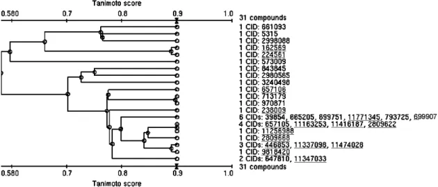
Figure 2.1b.6: The structural clustering of 15 mining hits from NCGC database combined with 16 AmpC beta-lactamase competitive inhibitors (underlined) based on the Tanimoto score. ...54

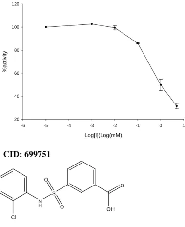
Figure 2.1b.7: The full dose response curve for compound 699751. ...54

Figure 3.1: A brief introduction to the PDBbind v. 2007………83

Figure 3.2: The pKd distribution of CSAR data sets (A. Set1; B. Set2). ...84

Figure 3.3: Illustration of the method to derive PL/MCT descriptors using the tesselated protein-ligand complex (3ERT, the ER/antagonists benchmarking dataset). ...85

Figure 3.4: The workflow of model building and validation using A) PDBbind data set; B) Set1 (solid line) or Set2 (dash-dotted line); C) PDBbind plus Set1 (solid line) or PDBbind plus Set2 (dash-dotted line). ...87

Figure 3.5: The statistics (R2, MAE, coverage, and RMSE; clockwise) of external n-fold validation sets using models built with A) Set1 (or Set2); B) PDBbind plus Set1 (or PDBbind plus Set2). ...89

Figure 3.6: Nearest neighbor distribution of Set1 as external set: A1) within itself; A2) based on neighbors taken from Set2 modeling set; A3) based on neighbors taken from PDBbind + Set2 modeling set. Likewise, nearest neighbor distribution of Set2 external set: B1) within itself; B2) based on neighbors from Set1 modeling set; A3) based on neighbors from PDBbind + Set1 modeling set. ...90

Figure 3.7: The 2D SPE plots. The black dots are data points of the external set and the red dots are data points of the modeling set. ...92

xiii

Figure 4.2: Illustration of the method to derive PL/MCT descriptors using the tesselated protein-ligand interface (e.g., 3ERT). ...124

Figure 4.3: Flowchart of the approach described in this paper for developing

target-specific pose filters, and their use in combination with MedusaScore for VS. ..125

Figure 4.4: The awROCE values at 1% (a) and awAUC values (b) of MedusaScore

(black) and MedusaScore + filter approach (dark green) for each target. ...126

Figure 4.5: The heat map of awROCE values at 0.5% (a) and 1% (b) of several popular structure-based scoring functions (XSCORE::HMSCORE, ChemScore, PLP, Chemgauss3, and MedusaScore) as well as MedusaScore plus Filter

approach for each target. ...127

Figure 4.6: The awROC curves of VS experiments for 13 DUD data sets. For each target, the true positive (FP) rate is plotted against the logarithmic false

positive (FP) rate. ...129

Figure 4.7: The analysis of ligand cluster type retrieval of MedusaScore + filter

xiv

List of Abbreviations

AD Applicability Domain

ADME Absorption, Distribution, Metabolism, Excretion

CCR Correct Classification Rate

CSAR Community Structure Activity Resources

CV Cross Validation

DFT Density Functional Theory

DUD Directory of Useful Decoys

EI Efflux Index

EN Electronegativity

EPI Efflux Pump Inhibitor

FEP Free Energy Perturbation

HTS High Throughput Screening

LIBSVM Library for Support Vector Machines

LIE Linear Interaction Energy

LMO Leave Multiple Out

LOO Leave One Out

MCT Maximal Charge Transfer

MDR Multiple Drug Resistance

MIC Minimum Inhibitory Concentration

MLR Multiple Linear Regression

NCE New Chemical Entity

xv

kNN k-Nearest Neighbors

PDB Protein Data Bank

PLS Partial Linear Squares

QSAR Quantitative Structure Activity Relationship

QSBAR Quantitative Structure Binding Activity Relationship QSPR Quantitative Structure Property Relationship

RMSD Root Mean Square Deviation

SAR Structure Binding Activity Relationship

SBDD Structure-based Drug Design/Discovery

SVM Support Vector Machines

TC Tanimoto Coefficient

Chapter 1 Introduction:

2

computational methods have been extensively applied in the drug discovery process with varying degree of success. This chapter will provide an overview of these technologies and some well-known limitations as well as the outline of this dissertation.

1.1 Cheminformatics in Drug Discovery

The term cheminformatics is firstly introduced in literature by Brown.9 Despite various extensions,10 broadly speaking, cheminformatics can be defined as: the application of informatics methods to solve chemical problems. Traditionally, the subjects in cheminformatics are mainly associated with small molecules despite the fact that macromolecules such as proteins and DNAs are also considered as chemicals. The research in understanding the relationship between macromolecules and ligands (mostly small molecules) is usually discussed intensively in the realm of structure-based drug design (Chapter 1.2).

3

molecules, helping to design new molecules, or identify molecules with desired property through searching chemical databases (i.e., database mining).

4

extension of ENTess descriptors – PL/MCT-tess descriptors – will be discussed in this dissertation (Chapter 3).

After completing the stage of data preparation, the next stage deals with the selection of techniques which optimize the correlation between desired property (dependent variable, Y) and molecular descriptors (independent variables, Xs) during model training. These optimization techniques can be generally divided into linear or non-linear, depending on whether the equation that is applied to explain the relationship between Y and Xs, is a linear combination of parameters or not. The most extensively applied linear method in QSAR studies is Partial Least Squares (PLS), which extends the traditional multiple linear regression (MLR) method when the number of independent variables (descriptors) is much larger than the number of data instances, a common situation in modern QSAR. However, as the increasing availability of experimental data resources, more and more compounds with diverse scaffolds are incorporated into QSAR modeling, the assumption that the variance of independent variables linearly corresponds to the variance of dependent variables is not always true. Instead, non-linear models may be constructed using machine learning algorithms such as k nearest neighbors (kNN). The kNN method is firstly introduced to QSAR world in 2000,17 where a particular compound’s property is predicted by its k nearest neighbors defined in a subset of descriptor space (resultants from the variable selection optimization).

5

models. The support vector machine (SVM) and random forest (RF) are among the most popular classification techniques. For example, the SVM algorithm searches for the optimal hyperplane that separates the two classes in the descriptor/feature space by maximizing the distance (called margin) between the classes' closest points. If the data is not linear separable in the descriptor space, the kernel trick is applied to project the data into higher dimensional feature space where the linear separation may exist.

6

single, “best” model. This could be resulted from the prediction error of compounds from one model cancelled by the correct predictions from the other model if the errors do not correlate. Furthermore, the compound should be predicted only when it is similar to the training set molecules (i.e., those within model applicability domain).18

Naming by the dimensionality of descriptors applied for model building, two types of QSAR methods, 2D-QSAR and 3D-QSAR are regularly compared to each other in many aspects such as the model performance and the ease of descriptor interpretation. Compared to 2D-QSAR models, 3D-QSAR models are more easily interpretable due to its visualizablity, making it simpler to suggest compounds for synthesis. The most popular commercial 3D-QSAR methods include Catalyst21 and Phase22. However, a recent study comparing these two programs demonstrates that the prediction accuracy of external validation set is less acceptable (the squared correlation coefficient, R2, less than 0.5), informing the further development of 3D-QSAR methodology is necessary.23 By contrast, our laboratory has been working on developing predicted 2D-QSAR workflow. Using predictive QSAR models as a virtual screening tool in hit discovery, many success stories are published.24-26 Herein, the QSAR binary classification modeling approaches are applied in several presented projects such as AmpC β-lactamase and Gram-negative efflux property (Chapter 2). And an extension of ENTess descriptors, P/L MCT-tess descriptors, is applied in QSBAR model building and structure-based virtual screening (Chapter 3 & Chapter 4).

1.2 Structure-based Drug Design

7

molecules, chemists could rationally design and optimize the lead molecules compared with time-consuming systematic modifications of molecular structures by cycles of trial-and-error. The 3D protein structural information can come from X-ray crystallography, NMR spectroscopy, cryo-electron microscopy, and homology modeling, where 3D protein structural model is constructed based on its amino acid sequence and a related homologous protein structure determined by experiments (e.g., x-ray crystallography). The popularity of SBDD has substantially increased in recent years since the first seminal paper was published in 1982 by Kuntz’s group.28 This mainly results from the remarkable technical advances in determining target protein structures and protein/ligand complexes, multiplying structural resources related to therapeutically relevant target proteins. The solved 3D structures may be deposited in Protein Data Bank (PDB)29, where researchers can freely search and download structures. The exponential increase of deposited PDB structures since 1980s (from 70 to 64,357 as of April 2010) also raises the quality issue of the applied structures in SBDD. Scrutinizing the congruence between the experimental electron density map and the fitted protein model gradually becomes a common and necessary procedure before any further SBDD calculations. Thus, various subdivided libraries of PDB are curated for such purpose. For example, PDBBind database30, 31 is curated by culling from high-quality protein-ligand complexes with experimentally measured binding affinity data. Nevertheless, SBDD approaches have been becoming indispensable tools in the early stage of drug discovery process.

8

protein binding site. This process involves several steps: a) search algorithms explore the possible binding regions for each compound within the target protein binding site and generate multiple poses; b) scoring functions are applied to calculate a score for each pose, which is represented the degree of complementarity to the binding site, or the predicted binding affinity; c) the best ranking pose is commonly selected to represent the binding of that particular compound (i.e., binding mode).

Since the pioneering docking program DOCK28, 32 published in 1980s, a series of other programs, such as FlexX,33 GOLD,34 and AutoDock35, have emerged. Each of them varies in the respect of pose generation algorithms, the applied scoring functions, and the degree of protein/ligand flexibility taken into account. At present, all docking programs allow compounds to dock flexibly, either by exploring the translational and orientational degrees of freedom of pre-generated conformers (e.g., Fred36), or by generating the poses on-the-fly (e.g., AutoDock). However, explicit protein flexibility (i.e., the movement of protein backbone/side-chain) is still not regarded as a norm in docking considering the size and possible degrees of freedom of macromolecule.

9

plethora of studies comparing the performance of different docking programs have been published.40-46 The 2006 GSK paper by Warren et al.47 concludes the current achieved status in docking by conducting an extensive retrospective study using ligand/decoy sets with experimentally determined binding affinities against a wide range of pharmaceutically relevant protein targets. In total, they evaluate 10 docking programs and 37 scoring functions and summarize the performance of those docking programs on three tasks: a) search algorithms in docking can generate poses which are closed to the experimentally determined binding mode (native pose) yet less successful in predicting the correct binding mode of ligands; b) docking/scoring can identify ligands among a set of pharmaceutically relevant decoys in virtual screening campaigns but the performance is highly target-dependent; c) in terms of lead optimization, none of the docking programs or scoring functions can make a useful prediction of ligand binding affinity. All of these retrospective studies demonstrate that significant improvements are needed for current scoring functions (or scoring schemes in virtual screening).

10

functions are designed based on various statistical parameters derived from x-ray crystal structures that could reflect the interactions between a ligand and its receptor depending on their molecular environment. Simple distance-dependent pair potentials and non-polar surface-dependent singlet-potential are used in DrugScore.52 They could implicitly capture the binding effects that are difficult to model in force field based scoring functions. Moreover, consensus scoring schemes53-56, which various data fusion approaches are used to combine information from multiple scoring results in the hope of compensating the errors inherent in each single score, are also widely employed. However, a paper published in 2005 demonstrates that consensus only works when each of the individual scoring functions has relatively high performance and the scoring characteristics of each individual scoring function are quite different.56

11

Recently, a hybrid (empirical + knowledge-based) scoring function incorporating the cheminformatics concepts into conventional structure-based scoring functions is developed in our laboratory.16 The scoring function is quantitative structure-binding affinity relationship (QSBAR) models constructed by 264 x-ray protein-ligand complexes with known binding affinity using ENTess descriptors. The ENTess descriptors are generated based on the tetrahedra resulting from Delaunay tessellation (Tess), characterizing the protein-ligand interface by means of Pauling electronegativity (EN) values. The output of ENTess scoring function can be directly related to absolute binding affinities and could implicitly take into account binding effects that are difficult to specify, combining the merit of both empirical and knowledge-based scoring function. However, the performance of ENTess scoring function in practical virtual screening is limited. One of the possible reasons could be the limitation in applicability domain of ENTess models. In Chapter 3, we report the study managing to improve the ENTess scoring function. .

12

discriminate native-like poses of ligands vs. pose decoys. The pose filter, along with MedusaScore (a force field-based scoring function), is combined to develop a novel two-step protocol for target-specific virtual screening with the aim to improve the hit enrichment in structure-based virtual screening.

1.3 Summary

This dissertation will describe the contributions to the field of SBDD by incorporating cheminformatics concepts into structure-based scoring methods. Firstly, cheminformatics practices are applied to those problematic cases which conventional structure-based scoring functions find difficult (anti-bacterial leads efflux study) or even fail to address (AmpC β -lactamase study). Secondly, novel pose and binding structure-based scoring functions and a two-step scoring protocol are developed by employing cheminformatics approaches to improve protein-ligand binding affinity prediction and structure-based virtual screening respectively.

Chapter 2 discusses two case studies demonstrating that cheminformatics approaches

can complement structure-based drug discovery/drug design and identify promising hits by virtually screening molecular libraries.

13

The second case study is differentiation of AmpC β-lactamase binders vs. binding decoys using the binary classification QSAR approach. The binding decoys are false positives mispredicted by conventional structure-based scoring functions. To differentiate them, I successfully construct predictive QSAR models based on rigorous internal and external validations. Applying the models to predict false positives and false negatives from high throughput screening, the models discard false positives and can rescue false negatives.

Chapter 3 explains the development of binding scoring function, which is a

collection of QSBAR models. Compared with the previous ENTess scoring function, the new binding scoring function is constructed with an increased number of protein-ligand complexes and novel protein-ligand interfacial descriptors incorporating conceptual DFT atomic properties. Upon the application of global applicability domain, this new binding scoring function shows acceptable prediction accuracy (the squared correlation coefficient: 0.57) towards the Community Structure-Activity Resources (CSAR) data set.

Chapter 4 describes the development of the target-specific pose (-scoring) filter with

the aim to improve the hit enrichment in structure based virtual screening. The pose filter is developed for each target by building binary classification models that can discriminate native-like poses of ligands vs. pose decoys. Furthermore, a two-step scoring protocol for target-specific virtual screening is developed. In the first step our pose filter is used to filter out/penalize putative pose decoys for every compound, and in the second step the remaining putative native-like poses are scored with MedusaScore, which is a conventional force-field-based scoring function.

Chapter 2 Cheminformatics Approaches Complement Structure-based Virtual Screening:

2.1a Classification of Gram Negative Bacteria Efflux Properties of Antibacterial Leads Using Pharmacophore Fingerprint-based SVM QSAR Modeling and Application to Virtual Screening

2.1a.1 Introduction

Bacterial multidrug resistance (MDR) is frequently reported in clinics, underlining the need for developing new antibiotics. Unfortunately, a majority of recently approved antibiotics and developing compounds still lack activities against Gram-negative bacteria despite the fact that they cover a number of novel, well-conserved bacterial targets to overcome the resistance by target modification and enzymatic drug inactivation. It is widely recognized that this intrinsic resistance largely results from the constitutive expression of multi-drug efflux pumps. Unlike other bacterial efflux pumps only selectively extruding specific drugs, efflux pumps involved in MDR can pump out a number of antibiotics with diverse structures and unrelated functions, rendering simultaneous bacterial resistance. The efflux issue is especially serious for Gram-negative bacteria due to combined effects of efflux pumps to actively expelling antibiotics (efflux) and the unique Gram-negative bacteria’s outer membrane to reducing antibiotics uptake (influx)70 (Figure 2.1a.1), providing an effective barrier against both hydrophilic and hydrophobic antibiotics.71

15

resistance nodulation division (RND) family. Among them, members in the RND family are the most significant efflux determinants of intrinsic and acquired resistance in Gram-negative bacteria. Efflux pumps in RND family are organized into three-component structures transversing both inner and outer membranes, allowing diverse antibiotic substrates to directly expel out from the cytoplasm and periplasm (Figure2.1a.1). Recent x-ray structures of efflux pumps co-crystallized with several ligands simultaneously in an extremely large cavity confirms the diverse substrate specificity of efflux pumps.73

The inhibition of efflux pumps has been suggested as a viable approach to overcome MDR. Common strategies for efflux inhibition include a) development of efflux pump inhibitors (EPI) in combination with available antibiotics to increase antibacterial potency; b) design of anti-bacterial lead compounds which can elude efflux pumps. The latter approach is potentially more practical compared to the former one, where EPIs can only be effective when the complimentary antibiotic substrates share the same binding site (i.e., competitive inhibition). One of the goals of this study is to help medicinal chemists to identify anti-bacterial lead compounds that can elude the efflux pumps using in silico models.

16

compounds).77, 78 Herein, in silico quantitative structure-activity relationship (QSAR) models are built to classify Gram-negative bacteria efflux properties (low vs. high) with five-fold external cross validation (CV) average accuracy as high as 79%. The predictive models are built and validated using GlaxoSmithKline (GSK) in-house pharamacophore fingerprint (pFP) descriptors and support vector machine (SVM) algorithm on a GSK proprietary K. pneumoniae efflux data set (~400 compounds). The models are subsequently applied in virtual high throughput screening and 60 out of 75 available potent computational hits are confirmed as low-efflux by bioassays, achieving high accuracy of 80%. The predictive models can also further be used to prioritize synthesis of GSK anti-bacterial series. These encouraging results provide a good template for further efflux modeling research.

2.1a.2 Methods

2.1a.2.1 Data Sets

The GSK anti-bacterial series are broad-spectrum bacterial topoisomerase IIa inhibitors

(Figure 2.1a.2), which show a novel mode of inhibition different from clinical

topoisomerase IIa inhibitors in the quinolone series, providing the hope of against topoisomerase IIa - mediated cross-resistance.79 However, the novel GSK anti-bacterial series also suffer from the multidrug efflux pump issue especially in Gram-negative bacteria.80 Thus, it is desirable to build in silico models to predict efflux properties of GSK anti-bacterial series to further improve potencies by reduction of efflux activities.

17

ratio of the MIC of wide-type bacteria to that of efflux knock out bacteria. The EI values are transformed to the logarithmic value (pEI) for modeling purpose (Equation 2.1).

(2.1)

Each MIC is measured at least twice to ensure data integrity. The experimental variability of pEI for each compound is usually around ±1, but could be as high as ±2. Therefore, a classification model is better suited for modeling the efflux indices. All compounds are classified by a threshold of pEC = 6, i.e. 64-fold difference between wide type MIC and efflux knock-out MIC, determined by biological interests. In total, there are 399 GSK anti-bacterial series annotated as low and high efflux properties against K. pneumoniae for modeling, containing 149 low-efflux compounds (37%) and 250 high-efflux compounds (63%). The pEI distribution of dataset is shown in Figure 2.1a.3. Compound structures are relatively diverse, including, for example, the tricyclic nitrogen series81 and the cyclohexane/cyclohexene series.82

Furthermore, seventeen compounds in a new subseries outside of training set are served as an additional external validation set. The pEI distribution of these 17 compounds is shown in Figure 2.1a.4.

Regarding the library used for virtual screening, a total of 4013 historical GSK bacterial topoisomerase IIa inhibitors without K. pneumoniae efflux properties are curated to search for low-efflux templates.

2.1a.2.2 Training, Test, and External Validation Set Selection

) MIC MIC ( log ) (

KO WT 2

=

18

The overall modeling workflow is shown in Figure 2.1a.5. The double five-fold cross validations are applied for modeling, including internal (optimization of model parameters) and external cross validations (testing model performance). The data set is randomly split into five subsets, where the ratio of low-efflux to high-efflux compounds corresponding to that in the modeling set. Each subset is applied independently to validate the models built from the remaining subsets by five-fold internal CV using the Support Vector Machines (SVM) algorithm. Furthermore, seventeen compounds in a new subseries outside of training set are served as an external validation set. The pEI distribution of these 17 compounds is shown in Figure 2.1a.4.

2.1a.2.3 Generation of Pharmacophore Fingerprint (pFP) Descriptors and

pFP Noise Reduction by pFPBitRank Tool

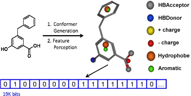
The GSK in-house pFP program is applied to generate the pFPs for all compounds. The implementation is similar to the one previously reported.83, 84 There are six pharmacophore feature types (hydrogen bond donor/acceptor, positive/negative ionizable, hydrophobic centroid, and aromatic centroid) and seven inter-pharmacophore distance bins (1.0-3.0, 3.0-4.0, 4.0-5.2, 5.2-6.5, 6.5-8.0, 8.0-10.0, 10.0-50.0, unit: Å). The distance bin boundaries are statistically determined to produce equal occupancies across a large set of GSK drug-like compounds. The combination of six pharmacophore feature types and seven distance bins leads to a total of 19208 pFP bits.

19

and stored into a bit string to generate per-conformer pFP (Figure 2.1a.6). All per-conformer pFPs of one compound at each pFP bit position are further processed by logical OR to generate the per-molecule pFP of that compound. As long as a certain three-point pharamacophore appears in any conformer, that bit is turned on in the per-molecule pFP. These three-point pharmacophore fingerprints are applied as descriptors to capture the physiochemical nature of a compound, as the GSK pFP descriptors have been successfully applied in both lead optimization and lead identification projects.85-87

The pFP BitRank tool 85 is applied to increase the signal to noise ratio in pFPs based on information from known low-efflux/high-efflux compounds. A score for each bit is calculated using Equation 2.2. Given the pFPs of sets of active (e.g., high-efflux) and inactive (e.g., low-efflux) compounds, each bit is scored according to relative prevalence amongst actives (a) or inactives (i)

BitScore(j) fa1 * fi0 + fa0 * fi1 (2.2)

where j is the id of each bit and fxy is the fraction of bits whose value is y (e.g., 0 or 1) amongst compounds in class x (e.g., active or inactive).

To estimate the “noise” bitscore value, the activity labels are shuffled (y-randomization) and the score for each bit is recalculated. This procedure is repeated 100 times and the mean as well as standard deviation are calculated using all bitscore values from randomization. Only the bits with bitscore higher than a certain Z cutoff are retained and applied as descriptors in SVM model building.

20

Here, is the average bitscore values from randomization, σ _{is the standard deviation of}

these bitscore values, and Z is an arbitrary parameter to control the significance level. (Further implementation details are not disclosed by GSK.)

2.1a.2.4 Support Vector Machine Classification Method

The Support Vector Machines (SVM) algorithm implemented in the open-source LibSVM88 package are employed to build binary classification models. The SVM algorithm searches for the optimal hyperplane separating the two classes in the descriptor space by maximizing the margin between the closest points of the two classes (Equation 2.3),

∑

=

+ l

i i T

C W W

1 2

1

min ξ , subject to i i

T

i W X b

y( Φ( + ))≥1−ξ (2.3)

where C is the penalty parameter and

ξ

0 ), exp(

) ( ) ( ) ,

( ≡Φ TΦ _i = −γ _i − _j γ >

i

j X X x x

x x

K (2.4)

where γ is the kernel parameter. We employ the Python script (grid.py) provided by LibSVM to optimize parameters C and γ during model building with 5-fold cross validation (CV). The search range of C and γ are -5 to 15 and -15 to 0 respectively.

2.1a.2.5 Virtual Screening Using pFP-SVM Models

All SVM models with eligible CV accuracy are used to predict the test set. When applied to the compounds in the test set of each fold CV, compounds are considered as low (or high) efflux only when they are predicted as low (or high) efflux consistently by no less

21

than 50% of all eligible models. However, in the VS study, a higher threshold (90%) is applied to select low-efflux compounds for experimental testing. A higher threshold is assumed to have higher confidence in prediction.

2.1a.3 Results and Discussions

2.1a.3.1 Relationship between Distribution Coefficient and Efflux Index

The correlation between the measured logD values (the logarithmic value of distribution coefficient) and the pEI values is analyzed based on the hypothesis that hydrophobic (i.e., high distribution coefficient) compounds tend to have higher EI values due to favorable interactions between hydrophobic compounds and the aromatic binding site of efflux pumps. As shown in Figure 2.1a.7, there is a marginal correlation between these two factors, indicating that efflux modeling is more complicated than simple polarity modeling. Therefore, extra structural information (e.g., pFP) is needed to build in silico efflux models.

2.1a.3.2 SVM Binary Classification Models

22

consensus prediction on the test sets. The overall statistics are summarized in Table 2.1a.1. The average prediction accuracy for training sets and test sets is as high as 76% and 79% respectively. The consensus models from the 1st fold and the 4th fold are applied to the additional external validation set and in the virtual screening.

2.1a.3.3 External Validations

Seventeen compounds in a new subseries outside of training set are served as an additional validation set for predictive models. Compounds are classified as low (or high) efflux only when they are predicted as low (or high) efflux consistently by no less than 50% of all eligible models. The prediction results are tabulated in Table 2.1a.2. Almost all low-efflux compounds (8 out of 12) are predicted correctly and three out of four false positives have pEI equal to 6 (i.e., borderline compounds).

In summary, validation results show that the pFP-SVM models can differentiate pharmacophore features of low-efflux compounds from high-efflux compounds and can be applied for virtual screening.

2.1a.3.4 Virtual Screening Using Predictive pFP-SVM Models

23

determined experimentally. For the remaining compounds (75 compounds), 80% are confirmed with low efflux properties.

2.1a.3.5 Virtual Screening Using LogD value

Further efforts are spent to investigate the prediction accuracy of using logD value alone to fish out the low-efflux compounds from those 75 compounds which could be assumed randomly selected from the library. The range of measured logD values of these 75 potent compounds is from -0.3 to 1.5. The probability of fishing out low-efflux compounds based on logD values lying in that range in the modeling set is 0.47 in comparison with the prediction accuracy (0.80) by using pFP-SVM models, demonstrating the benefits of QSAR modeling of efflux properties.

2.1a.4 Conclusions

Figures for Chapter 2.1a

Figure 2.1a.1: Schematic representation of both the inner and outer membrane of Gram

negative bacteria together with the porous layer of peptidoglycan, the main target of beta lactam antibiotics (in blue).

Influx and efflux systems are also inserted to show the uptake a antibiotics. The figure is modified from the Figure (1) in

24

Schematic representation of both the inner and outer membrane of Gram negative bacteria together with the porous layer of peptidoglycan, the main target of beta

Influx and efflux systems are also inserted to show the uptake and suggested extrusion of antibiotics. The figure is modified from the Figure (1) in Curr Drug Targets.

Schematic representation of both the inner and outer membrane of Gram-negative bacteria together with the porous layer of peptidoglycan, the main target of

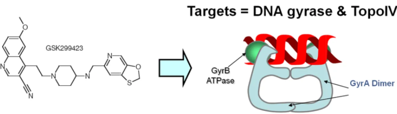
Figure 2.1a.2: The novel GSK antibiotic series target bacterial topoisomerase IIA (DNA

gyrase and topo IV).

The inhibition mechanism of GSK bacterial topoisomerase IIA inhibitors is different from the one of fluoroquinolones, circumventing the topoisomerase IIa

Figure 2.1a.3: The distribution of pEI

Applying pEI, 6, as the threshold, totally, there are 149 low 250 high-efflux compounds (Red).

0

50

100

150

200

2-4

4

10

139

#

o

f

C

o

m

p

o

u

n

d

s

Distribution of

25

The novel GSK antibiotic series target bacterial topoisomerase IIA (DNA

The inhibition mechanism of GSK bacterial topoisomerase IIA inhibitors is different from the one of fluoroquinolones, circumventing the topoisomerase IIa - mediated cross

The distribution of pEI values of the GSK bacterial topoisomerase IIa dataset. Applying pEI, 6, as the threshold, totally, there are 149 low-efflux compounds (Green) and

efflux compounds (Red).

4-6

6-8

8-10 >10

139

196

47

7

pEI

Distribution of pEI

The novel GSK antibiotic series target bacterial topoisomerase IIA (DNA

The inhibition mechanism of GSK bacterial topoisomerase IIA inhibitors is different from mediated cross-resistance.

Figure 2.1a.4: The distribution of pEI

structure activity relationship (SAR) with single functional group substitution of GSK antibiotics series.

There are nine low-efflux compounds (Green), three borderline compounds (yellow), and five high-efflux compounds.

Figure 2.1a.5: The workflow of efflux model building, validation, and virtual screening.

3

5

<6 =6

Distribution

of

26

The distribution of pEI of the newly synthesized compounds by exploring structure activity relationship (SAR) with single functional group substitution of GSK

efflux compounds (Green), three borderline compounds (yellow), and flux compounds.

The workflow of efflux model building, validation, and virtual screening.

9

=6 <6

of pEI

of the newly synthesized compounds by exploring structure activity relationship (SAR) with single functional group substitution of GSK

efflux compounds (Green), three borderline compounds (yellow), and

Figure 2.1a.6: The pFP descriptor calculation. For each compound, multiple conformers are

generated, each of which is assigned Along with seven distance bins (1.0

unit: Å), the 19208 three-point phamacophore features constraint and stored into a bit string.

27

descriptor calculation. For each compound, multiple conformers are generated, each of which is assigned six pharmacophore features.

distance bins (1.0-3.0, 3.0-4.0, 4.0-5.2, 5.2-6.5, 6.5-8.0, 8.0

point phamacophore features are enumerated based on the triangle constraint and stored into a bit string.

descriptor calculation. For each compound, multiple conformers are

28

29

Tables for Chapter 2.1a

Table 2.1a.1: The statistics of accuracies from internal and external five-fold cross-validation (CV) by models with internal CV accuracy larger than 75%.

CV split Average CV accuracy (%)

Test set accuracy (%)

Low efflux accuracy (%)

High efflux accuracy (%)

# of models w/ accuracy ≥ 75%

#1 75 84 71 91 50

#2 75 80 76 82 17

#3 76 78 71 84 20

#4 78 76 65 82 100

#5 75 77 63 82 6

Table 2.1a.2: The confusion matrix of 17 newly synthesized compounds with single functional group substitution.

predicted experimental

Low (pEI <=6) High (pEI > 6)

Low (pEI <6) 8 1

Borderline (pEI = 6) 0 3

30

2.1b Differentiation of AmpC β-Lactamase Binders vs. Binding Decoys Using Classification

k-NN QSAR Modeling and Application of QSAR Classifier to Virtual Screening

2.1b.1 Introduction

Due to rapid advances in protein crystallography90, 91, the number of x-ray characterized biological targets and their complexes with various low molecular weight ligands in the RCSB Protein Data Bank (PDB)29 has been growing rapidly. This growth has been concurrent with the development of a vast array of structure-based virtual screening approaches 92-101. These methods include two critical components, i.e., docking and scoring. It has been shown that multiple binding poses of putative receptor ligands resulting from docking include those that are geometrically close to the native (i.e., experimental) ligand orientation in the binding site. However, identifying (the most) native-like binding poses among many alternatives (i.e., ‘geometrical decoys’) resulting from docking continues to present a universal problem to most scoring functions.47, 102, 103 Furthering this problem is a demonstrated inability of many scoring functions to discriminate between ligands that are known to bind to the target receptor from those known to be non-binders yet predicted to bind by a docking/scoring method (so called ‘binding decoys’) 42, 104.

31

validation. Similar results have been observed for several other systems (available from the B. Shoichet’s laboratory website, http://shoichetlab.compbio.ucsf.edu/take-away.php).

32

The goal of this study was to develop robust binary classification QSAR models that would have high predictive power to differentiating binders vs. non-binding ‘decoys’ for AmpC beta-lactamase. We have employed a rigorous validated QSAR modeling workflow that has been developed in our laboratory in recent years. This workflow that incorporates a virtual screening module was applied successfully to several ligand datasets leading to the identification of experimentally confirmed novel hits for different biological targets 112-116 (see recent review 117 ). Herein, we report on classification QSAR models that are capable of discriminating binders from decoys with the external classification accuracy exceeding 90%. Furthermore, we have used these models to screen the compound library tested earlier in the AmpC assay and available from PubChem 118. We have identified 15 molecules as putative AmpC ligands and demonstrated in subsequent experimental studies that five compounds chosen from these hits were millimolar binders. It worth emphasizing that in all studies reported in this paper we did not use any information on the crystallographic structure of AmpC-ligand complexes and moreover, chemical descriptors were generated from two-dimensional rendering of molecular structures.

2.1b.2 Methods

2.1b.2.1 Data Sets

Compounds used for QSAR model building.

The AmpC beta-lactamase inhibitors and binding decoys were downloaded from Dr. Brian Shoichet’s laboratory web site 119. This dataset contains 21 confirmed inhibitors (cf.

33

Library used for virtual screening.

We used the dataset of 69653 compounds that was screened in the HTS assays for AmpC beta-lactamase inhibition by the National Center for Chemical Genomics (NCGC). The screening results are reported in PubChem as Bioassays AID584 123 and AID585 124. The experimental protocols are described in 125 as well as in the PubChem database. AID584 and AID585 were designed for screening of specific and promiscuous AmpC beta-lactamase inhibitors, respectively. Compounds are classified as having full titration curves, partial modulation, partial curve (weaker actives), single point activity (at highest concentration only), or inactive. Compounds that showed activity in both AID584 and AID585 assays were considered ‘true’ positives. However, if compounds were only found active in AID585 but inactive in AID584, they were categorized as ‘aggregators’. Thus, 64 compounds were identified as ‘true inhibitors of’ the AmpC beta-lactamase that could be used to test the ability of QSAR model based virtual screening to recover known hits.

2.1b.2.2 AmpC β-lactamase Competitive Inhibitor Assay

The details of enzymatic assays to measure the efficiency of AmpC beta-Lactamase inhibitors were described in detail elsewhere (26, 40). Briefly, the change in initial rate of substrate hydrolysis at increasing concentrations of the inhibitor was monitored and the IC50 was obtained using the resulting dose-response curve. The inhibition constant, Ki, was derived from the IC50 value using the Cheng-Prusoff equation.

2.1b.2.3 Training, Test, and External Validation Set Selection

34

For classification QSAR modeling, it would be ideal to have the balanced ratio between different compound classes in the modeling dataset. However, the AmpC beta-lactamase binding dataset included 21 inhibitors and 80 decoys, i.e., it is imbalanced with the inhibitors to non-binders ratio of 1:4. In the absence of special statistical treatment, such ratio would skew the prediction accuracy of the classification models. Thus, the distance matrix was calculated in the multidimensional descriptor space for all 101 compounds and similarity search was carried out using 21 inhibitors as queries against the remaining 80 non-binders. 30 compounds were selected from the original 80 non-binders as most similar to 21 inhibitors using Euclidean distance as similarity metric (we note that this treatment makes the task of building the discriminatory binary QSAR models even more challenging. Consequently, these 30 non-binders combined with 21 true inhibitors formed a new balanced dataset for QSAR model building. The remaining 50 “dissimilar” non-binders were retained as an external validation set. Furthermore, 10 compounds (five binders and five decoys) were randomly excluded from the balanced dataset of 51 compounds and formed a second external validation set. The remaining 41 compounds were considered a modeling dataset that was divided into multiple diverse and representative training and test sets using the Sphere Exclusion approach developed in our laboratory earlier 20, 126.

2.1b.2.4 Generation of 2D Molecular Descriptors

The SMILES 127 strings of each compound in AmpC beta-lactamase dataset were converted to 2D chemical structures using the Unity module of the SYBYL software package 128

35

connectivity indices 130-132, kappa molecular shape indices 133, 134, topological and electrotopological state indices 135-137, differential connectivity indices,graph’s radius and diameter 138, Wiener and Platt indices, Shannon and Bonchev-Trinajstić information indices, counts of different vertices, counts of paths and edges between different kinds of vertices.

Overall, MolConnZ produced over 770 different descriptors. Most of these descriptors

characterize chemical structure, but several depend upon the arbitrary numbering of atoms in a

molecule and are introduced solely for bookkeeping purposes. In our study, only 644 chemically

relevant descriptors were initially calculated and 340 descriptors were eventually used for AmpC

beta-lactamase binding dataset after deleting descriptors with zero value or zero variance. MolConnZ

descriptors were range-scaled prior to distance calculations since the absolute scales for MolConnZ

descriptors can differ by orders of magnitude139. Accordingly, our use of range-scaling avoided giving

descriptors with significantly higher ranges a disproportional weight upon distance calculations in

multidimensional MolConnZ descriptor space.

2.1b.2.5 k-Nearest Neighbors (k-NN) Classification Method

36

∑

∑

ˆ (1)

where k is the number of nearest neighbors (k = 1 to 5) of compound i, yj is the class

membership of compound j and dij is the Euclidean distance between compound i and its jth

nearest neighbors. In practice, the value of yˆ is rounded to determine the class membership _i of compound i:

i

yˆ = round (' yˆ ) (2) _i

The model is internally validated by leave-one-out cross-validation (LOO-CV) where each compound is eliminated from the training set and its class membership is predicted as the class the majority of its k nearest neighbors belongs to. The descriptor set is optimized by simulated annealing approach with the Metropolis-like acceptance criterion to achieve the best CCR value. The CCR is defined as113:

CCR = 0.5(TP/N1+TN/N0) (3)

37

number of nearest neighbors, and a subset of selected descriptors. Additional details of this approach can be found elsewhere139, 141.

2.1b.2.6 Applicability Domain of k-NN Models

When developing kNN QSAR models, each compound is represented as a point in M-dimensional descriptor space (where M is the total number of selected descriptors); thus, the molecular similarity between any two molecules can be characterized by the Euclidean distance between their representative points. The Euclidean distance di,j between two points i

and j (which correspond to compounds i and j) in M-dimensional space can be calculated as follows:

∑

−

= M

k

jk ik

ij X X

d

1

2

)

( (4)

Compounds with the smallest distance between one another are considered to have the highest similarity.

38

DT = + Zσ (5)

Here, is the average Euclidean distance of the k nearest neighbors of each compound within the training set (where the value of k is the same as in predictive kNN QSAR models),

σ _{is the standard deviation of these Euclidean distances, and Z is an arbitrary parameter to}

control the significance level. Typically, we set Z to 0.5, which places the boundary for deciding whether a compound is within or outside of the applicability domain at one-half of the standard deviation. It is important to notice that increasing the value of Z would increase the number of compounds in the external set that are considered within the applicability domain but could decrease the accuracy of prediction due to inclusion of dissimilar nearest neighbors.

2.1b.2.7 Y-randomization Test

Y-randomization test is widely used to ensure model robustness 142. It includes rebuilding the training set models using randomized activities (Y-vector) of the training set and comparing the resulting model statistics with that for the original test set. It is expected that models built with randomized activities should have significantly lower CCR value for both the training and test sets. In the model building process, it is possible that sometimes, though infrequently, high CCR values may be obtained due to a chance correlation or structural redundancy of the training set. If QSAR models obtained in the Y-randomization test have relatively high LOO-CV CCRtrain as well as predictive CCRtest, it implies that acceptable QSAR models cannot be obtained for the given dataset by the current modeling method. In this study, the Y-randomization test was performed twice for each training/test set splits.

y

39

2.1b.2.8 Virtual Screening using k-NN Models

As mentioned above, the screening database included 69653 compounds tested by the NCGC against AmpC beta lactamase. The primary HTS screening assay identified 64 “true” hits. Thus, we chose to screen the same database in silico using QSAR models as predictors. Only QSAR models that passed both internal and external validation tests were used. For each model we retained its parameters established in the process of external validation, i.e., the number of nearest neighbors k, selected descriptors, and Zcutoff value for the applicability domain.

2.1b.3 Results and Discussions

2.1b.3.1 k-NN Binary Classification Models

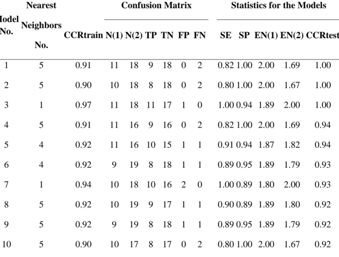
As shown in Figure 2.1b.2, the kNN QSAR method with variable selection afforded multiple models with optimal accuracy characterized as CCR for both training and test sets. In total, there were 3305 models with both CCRtrain and CCRtest equal or higher than 0.70. Most models with CCRtest ≥ 0.70 also had corresponding CCRtrain ≥ 0.70, but the opposite was not always true. The models with high values of both CCRtrain and CCRtest (≥ 0.70) were considered acceptable. 342 predictive models with the highest values of CCR (CCRtrain and CCRtest >= 0.90, red dots in Figure 2.1b.2) were selected for consensus prediction. Table

40

method was generally successful in correctly distinguishing binders vs. decoys using MolConnZ chemical descriptors of compounds only.

2.1b.3.2 QSAR Model Validations

In addition to the internal validation of kNN models using test sets, Y-randomization and external validation are the critical steps of the entire QSAR workflow (Figure 2.1b.1). Only models that have been validated by these two steps can be utilized for external prediction and database mining 19.

Y-randomization Test

In Y-randomization test, the binary annotations of AmpC beta-lactamase as inhibitors or non-binders were randomly shuffled and kNN classification models were built with the same parameter setting. The test was performed twice and both runs of Y-randomization tests showed that there were relatively small numbers of 330 and 429 models having both CCRtrain and CCRtest higher than 0.70. However, there were no models with both CCR value higher than 0.90. It implied that the kNN models obtained with real binding affinities and CCR greater than 0.90 are robust.

External Validation

41

leading to CCR = 1.00, SE = 1.00, SP = 1.00, EN(1) = 2.00, and EN(0) = 2.00. The accuracy of prediction for 50 non-binders was also high, ranging from CCR = 0.87 under Zcutoff = 0.5 to CCR = 0.86 under Zcutoff = 3.0 (Table 2.1b.2). Because of the applicability domain inherent to individual kNN QSAR models, the consensus prediction usually can not cover the whole dataset. By increasing the Zcutoff from 0.5 to 3.0, the prediction coverage for 50 non-binders increased from 94% to 98% whereas the prediction accuracy decreased. Figure

2.1b.3 shows the consensus scores and the coverage of predictive models for each of the 50 non-binders. The consensus score, in terms of the average class number in classification QSAR, was calculated by the fraction of models that predicted a compound as non-binder over the total number of models used for prediction plus 1. Under Zcutoff = 0.5, six falsely predicted inhibitors (average class number < 1.5) were within the applicability domain of only 70 models (i.e., approximately 20% of all models), i.e., the model coverage was as low as 20%. In general, the prediction with such a low coverage is viewed as of low confidence level. The higher Zcutoff significantly raised the model coverage for both inhibitor and non-binder prediction because of the extended applicability domain for individual models. In

Figures 2.1b.3B and 2.1b.3C, the model coverage for predicting inhibitors jumped up to 53% for Zcutoff = 1.5 and up to 94% for Zcutoff = 3.0. However, the prediction with extended applicability domain for consensus models also comes with lower confidence level. Generally speaking, in order to have the reliable and accurate prediction, one has to have the broader model coverage and a smaller Zcutoff value.

42

prediction had relatively small Zcutoff (= 0.5) and relatively broad coverage for compounds in external datasets (>= 50%).

2.1b.3.3 External Prediction

We used models built from 41 AmpC inhibitor/nonbinder dataset to verify the 64 "actives" from AID 584 and AID 585 screening. Under Zcutoff = 0.5, we could only generate predictions for 25 compounds out of 64 "actives" whereas the remaining compounds were found to be outside of the applicability domain. As shown in Table 2.1b.2, five out of these 25 compounds were predicted as true inhibitors. However, the predictions were based on only two models (out of 342 models with both CCRtrain and CCRtest higher than 0.90, cf.

Figure 2.1b.4A). Thus, the coverage for both compounds and consensus models was extremely low and as a result these predictions should not be viewed as reliable. Even under higher Zcutoff = 3.0, the model coverage was still low such that "actives" were predicted by only 110 models (32% of all models, cf. Figure 2.1b.4C). Furthermore, the formal prediction accuracy (assuming that the 64 hits were true inhibitors) was extremely low, e.g. CCR = 0.20 (Zcutoff = 0.5), CCR = 0.10 (Zcutoff = 1.5) and CCR = 0.15 (Zcutoff = 3.0) (Table 2.1b.2). Thus, based on our modeling results none of the 64 compounds in the NCGC set was predicted reliably as a non-covalent and reversible inhibitor.

43

confirmed yet but preliminary data indicate that none of them act as true reversible inhibitors of beta-lactamase (Dr. Shoichet, personal communications). These recent results confirm that our models are both accurate and robust.

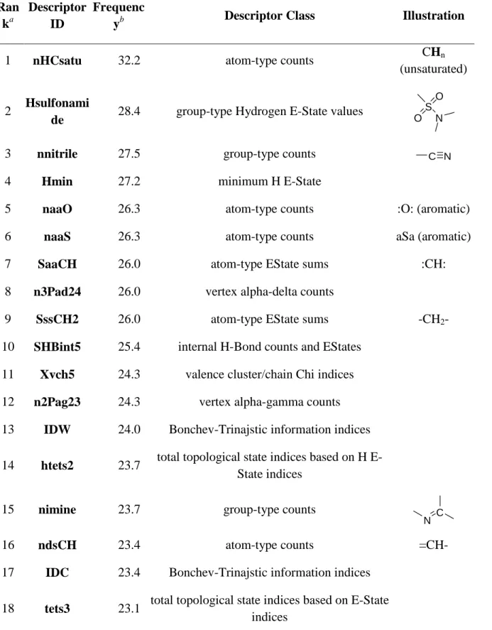
2.1b.3.4 Descriptor Interpretation

44

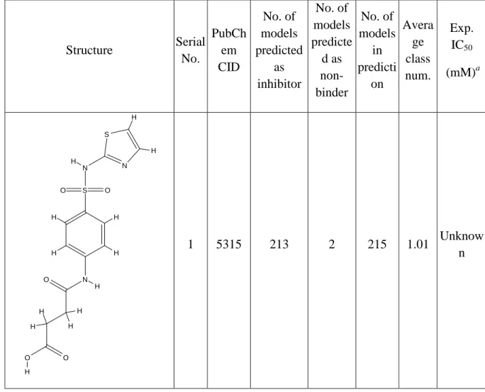
2.1b.3.5 Virtual Screening Using Predictive QSAR Models

Instead of using only one single and best model for virtual screening, the consensus prediction approach was applied that relies on averaging predictions from all qualified models, i.e. 342 models with both CCRtrain and CCRtest equal to or greater than 0.90. The complete modeling set (i.e., including training and test sets) was used for the prediction using each model as opposed to using only the corresponding training set. Initially, as many as 4565 compounds in the NCGC dataset of 69653 compounds were predicted as inhibitors by at least one of 342 models. To narrow the hit list and obtain the higher confidence level for each prediction, we took both the consensus score (average class number) and model coverage into account. In particular, only the hits with average class number between 1.0 and 1.2 and the model coverage over 50% (171 out of 342 models) were selected (Figure 2.1b.5). Furthermore, we restricted ourselves to the most conservative applicability domain for each model using Zcutoff = 0.5. We found that there were only 15 compounds that satisfied both criteria (Table 2.1b.4).