The Efficient Application of Automatic Differentiation for
Computing Gradients in Financial Applications
∗Wei Xu1, Xi Chen2 and Thomas F. Coleman3 1 Department of Mathematics, Tongji University
Shanghai, China, 200092
2 Department of Statistics and Operations Research, University of North Carolina
Chapel Hill, NC, USA
3 Department of Combinatorics and Optimization University of Waterloo
Waterloo, On. Canada, N2L 3G1.
1 [email protected] 2[email protected] 3[email protected]
July 31, 2014
Abstract
Automatic differentiation is a practical field of computational mathematics of growing interest across many industries, including finance. Use of reverse-mode AD is particularly interesting since it allows for the computation of gradients in the same time required to evaluate the objective function itself. However, it requires excessive memory. This memory requirement can make reverse-mode AD infeasible in some cases (depending on the function complexity and available RAM) and, in others, slower than expected due to use of secondary memory and non-localized memory references. On the other hand, it turns out that many complex (expensive) functions in finance exhibit a natural “substitution structure”. In this paper, we illustrate this structure in computational finance arising in calibration and inverse problems, as well as determining Greeks in a Monte Carlo setting. In these cases the required memory is a small fraction of that required by reverse-mode AD but the computing time complexity is the same. In fact, our results indicate significant realized speedup over straight reverse-mode AD.
Key words: Gradient, Automatic differentiation, Reverse-mode, Greeks, Local volatility, Calibration, Inverse Problems, Algorithmic Differentiation, Monte Carlo method.
∗This work was supported in part by the Ophelia Lazaridis University Research Chair (held by Thomas
1
Introduction
Many applications in finance require the efficient computation of gradients. For example, first-derivatives of pricing functions of options (i.e., “Greeks”), are required for hedging op-erations. As another example, calibration of complex models typically requires gradients of a regression function. More generally, minimization of functions of groups of pricing functions requires the computation of gradients at many points. Speed and accuracy are often paramount in these applications and the new discipline of automatic differentiation (AD)[21] offers a promising solution. Indeed, since it is known that in principle the reverse-mode of automatic differentiation can yield accurate gradients in time proportional to the time required to evaluate the objective function itself, it appears that a complete solution is at hand. In fact, several authors have made this connection in the context of determining Greeks in a Monte Carlo setting [7, 9, 10, 19].
In 2006, Giles and Glasserman [19] applied AD to calculate Greeks of interest rate deriva-tives priced by the Libor market model. Subsequently, the application of AD to compute Greeks of financial derivatives has gained the attention of academia and industry. Leclerc, Liang and Schneider [24] utilized reverse-mode AD to calculate the sensitivities of receiver Bermudan swaption with Libor market model. Their pricing framework is based on Monte Carlo simulation with Longstaff-Schwartz regression to determine the timing of early ex-ercise while Joshi et al [27, 25, 26] applied AD with the Libor Market Model in different contexts. In [28], Kaebeat alproposed a method based on adjoint methods (reverse mode) to speed up the Monte Carlo based calibration of financial market models. The adjoint method is applied to compute derivatives efficiently, rather than the finite difference method, but the massive memory storage issue is not considered in [28]. Recently, AD was also applied to analyze the sensitivity of credit derivatives, such as CODs and CDS’s, and manage the credit risk [8, 5]. Capriotti and Giles [9, 10, 6]discussed the computation of correlation Greeks for basket default swaps, CDOs and counterparty risk of credit portfolios through reverse-mode AD. However, the credit derivative payoff functions usually are not contin-uous. This discontinuity may cause biased estimators produced by the direct application of AD. Some adjustment techniques on payoff functions were proposed in [9, 10, 6] when computing sensitivities of CDOs and CDS’s. Compared with the forward mode (finite differ-ence method), the reverse-mode is efficient from the computational complexity point of view.
are structured and hence this structured approach can be usefully applied in finance, pro-viding a practical, accurate way to compute gradients in finance, efficient in space and time.
First we recall the following AD complexity results. Assume that F : Rn → Rm is a differentiable map. Let V ∈ Rn×tV. We denote the number of operations (a measure of
time) to evaluate a functionF at an arbitrary point, given a code forF, asω(F); we denote the space used by the given code to evaluate F as σ(F). Then forward-mode AD can be applied directly to functionF with matrixV to yield the productJ·V in time proportional to tV ·ω(F), and space proportional to σ(F) [21, page 36]. Similarly, ifW ∈Rm×tW then
reverse-mode AD can be applied directly to functionF with matrixW to yield the product
WTJ in time proportional totW·ω(F) and space proportional toω(F) [21, page 44]. (Note
that reverse-mode AD has a significantly increased demand for space over forward mode AD; typically, ω(F)≫σ(F).) When m < n reverse-mode AD is faster than forward-mode, at least in principle.
A special case of computing Jacobian products is when V = I and then these complex-ity results indicate that the Jacobian can be obtained by forward mode in timen·ω(F) and space σ(F); alternatively, if W =I then the Jacobian can be determined by reverse-mode AD in time m·ω(F) and space σ ∼ ω(F). We note that the sparse Jacobian case can be more efficient in time complexity: a combination of forward and reverse-modes can be used to get the Jacobian matrix in time χ(J) ·ω(F) where χ(J) is a measure of sparsity. In many cases χ(J) ≪ min(m, n) [12, 15, 31]. In this paper we are concerned with gradient determination, and som= 1, and these sparsity issues have little direct bearing.
Previous work addresses the problem of the extensive memory requirements of reverse-mode AD [4, 21]. Most of this work can be described under the banner of a computer science technique known as “checkpointing” [20]. Checkpointing is a general procedure that can be defined on a computational graph of a function to evaluate and differentiate an arbitrary differentiable functionz=f(x), where for convenience we restrict our discussion to a scalar-valued function ofn-variables, i.e.,f :Rn→R. The general idea is to cut the computational graph at a finite set of places (checkpoints) in a forward evaluation of the function f(x), saving some state information at each of those checkpoints and then recompute the informa-tion between checkpoints in a backward sweep in which the derivatives are computed. The advantage is potentially considerable savings in required space (compared to a reverse-mode evaluation of the gradient which requires saving the entire computational graph). There is some computing cost - but the total cost is just a constant factor times the cost to evaluate the function (i.e., the cost to perform the forward sweep). So this checkpointing procedure is the same order of work as straight reverse-mode AD but considerably less space.
to store [29]. Examples of checkpointing manifestations are included in [23]. Typically the user of the checkpointing idea either has to explicitly, in a “hands-on” way, decide on these questions for a particular application, or allow a checkpoint/AD tool to decide. There is no “well-accepted” automatic way that we know of to choose optimal checkpoints, and choice of checkpoint location clearly matters. The authors in [11] have done some work on this matter, with reference to determining general Jacobian matrix: one conclusion is that it is very hard to choose an ideal set of checkpoints in an automatic way, given the code to evaluate f(x). Some AD software apparently does decide automatically on checkpoint location (and state variable to save) though the actual rules that are used are, in our view, somewhat opaque.
Our proposed technique in this paper can be categorized as a particular (and practical) manifestation of checkpointing. Specifically, it is illustrated that many practical applica-tions (in finance) have a particular structure (see (2.1)) and if this structure is explicitly exposed in the function presentation then a natural set of checkpoints is evident and the set of state variables that are needed to allow for the backward sweep is also clear (and of relatively modest size).This observation is of considerable practical value. The contribution of this paper therefore has these two major dimensions: observing and illustrating that many applications in finance have this general structure (2.1), for relatively small ‘p’, and given that a function is presented in this structured form detailing an explicit well-defined way to deploy the checkpointing idea to compute the gradient.
The rest of this paper is organized as follows. In Section 2, we discuss the basics of au-tomatic differentiation and this practical notion of structure and how it can yield significant efficiencies. In the subsequent Section 3 and 4 we consider two common but distinct settings in computational finance: gradient computation to help in the determination of volatility surfaces, and the Monte Carlo evaluation of options (and subsequent computation of Greeks). These are broad example settings to illustrate how structure can be used, in computational finance, to enable efficient gradient computation. Results of some numerical experiments are presented in Section 5 that show the memory and realized computational time saving through the structured gradient computation. Finally, we conclude with some observations in Section 6.
2
Calculating Gradients of Structured Functions
We consider the following structured form. To evaluate a scalar-valued functionf(x) suppose that the procedure is:
Solve for y1 : T1(x)−y1 = 0 Solve for y2 : T2(x, y1)−y2 = 0 ..
.
Solve for yp : Tp(x, y1, y2,· · ·, yp−1)−yp= 0
Solve for z: ¯f(x, y1, y2,· · ·, yp)−z= 0.
The intermediate values, yi,i= 1,· · ·, pare, in general, vectors of varying length; functions
Ti, ¯f are differentiable functions of their arguments.
The corresponding extended Jacobian, i.e., Jacobian of (2.1) with respective tox, y1,· · ·, yp,
can be written in a partitioned form
JE =
J1
x −I
Jx2 Jy21 −I
..
. ... ... . ..
Jxp Jyp1 ... J
p
yp−1 −I
∇f¯T
x ∇f¯yT1 · · · · · · ∇f¯
T yp = A B
∇f¯T
x ∇f¯yT
. (2.2)
Then, the gradient off, with respect to x, satisfies [12, 15]
∇fT =∇f¯xT − ∇f¯yTB−1A (2.3)
The key to this approach is this: It is not necessary to explicitly compute matrices (A, B)
in order to compute ∇fT given by (2.3). Specifically, the off-diagonal submatrices in(A, B)
involved in the calculation of (2.3) occur only in a product form consistent with effective “just in time” application of reverse-mode AD.
To understand the algorithm given below, consider the following approach to the computa-tion of vT =∇f¯yTB−1A. We can define wT = (w1T,· · ·, wpT) to satisfywT =∇f¯yTB−1 in a transposed form
−I (Jy21)T (Jy31)T · · · (Jyp1−1)
T (Jp y1)
T
−I (Jy32)T · · · ... (Jyp2)
T
−I · · · ... ...
. .. (Jypp−−12)
T Jp yp−2
−I Jypp−1
−I w1 w2 w3 .. .
wp−1
wp =
∇f¯y 1
∇f¯y 2
∇f¯y 3 .. .
∇f¯y
p−1
∇f¯y
p (2.4) and
vT =∇f¯yTB−1A=wTA=wT1Jx1+w2TJx2+· · ·+wpT−1Jxp−1+wpTJxp. (2.5) Thus, we have the following algorithm to compute the structured gradient in (2.3).
Algorithm 1 Algorithm for Structured Gradient
1. Following (2.1) evaluate the values of y1, y2, · · ·, yp only.
2. Evaluatez= ¯f(x, y1,· · ·, yp)and apply reverse-mode AD to obtain∇f¯T = (∇f¯xT, ∇f¯yT1,· · ·,∇f¯
3. Compute the gradient using (2.4).
(a) Initialize vi= 0, i= 1 :p, ∇f =∇f¯xT, (b) For j=p, p−1,· · ·,1
wj =∇f¯yj−vj;
- Evaluate Tj(x, y1,· · ·, yj−1) and apply reverse-mode AD with vectorwTj to get
wTj ·(Jxj, Jyj1,· · ·J
j
yj−1). Setv
T
i =viT +wTj ·J j
yi for i= 1,· · ·, j−1; -Update ∇fT ← ∇fT +wTjJxj;
Note that Step 1 takes time proportional to ∑pi=1ω(Ti) ≤ω(F) and space proportional to
σ(F) while Step 2 requires time proportional toω( ¯f) and space proportional toω( ¯f). When
∇fT is updated in Step 3, its work is proportional to ∑pi=1ω(Ti) ≤ω(F) and the required
space satisfiesσ≤max{ω(Ti), i= 1,· · ·, p}. Thus, the theoretical time required to evaluate
the gradient by this structured approach is proportional to ω(f) , similar to reverse-mode AD, but the space required satisfies σ ≤max{ω(Ti), i = 1,· · ·, p, ω( ¯f)}, which compares
very favorably to ∑pi=1ω(Ti) +ω( ¯f), the space required by reverse-mode AD.
This greater space efficiency not only implies that our proposed method will apply to a wider set of problems (i.e., before exhausting all available RAM) compared to direct appli-cation of reverse-mode AD, but also results in better realized running times, due to localized memory reference. The results in Section 5 support this claim.
3
Nonlinear inverse problems, calibration, volatility surfaces
The problem of estimating a volatility surface, given a set of option prices on the same un-derlying, is an important and well-studied problem [13]. It is, in style, an engineering design problem formulated as a nonlinear inverse problem. Such problems are usually expressed as minimization of a regression function; most numerical approaches to such problems in-volve the determination of the gradient of the regression function. The AD technique for gradients of structured functions come into play here and can yield very efficient gradient determination. We note that these problems are often large and expensive because of the required approximation of a PDE model. Calculation of the gradient can be a non-trivial, expensive task.
The general discretized setting can be described as follows. Let x ∈ Rn be the vector of problem parameters, sometimes called control variables, and now (temporarily) assume that we have fixed the parameters x = ¯x for some specified values ¯x . Suppose y ∈ Rp is the vector representing the state of the system given the parametersx= ¯x. Specifically,yis the solution to theforward problem,
Typically function ˜F is a square continuously differentiable mapping, sendingp-vectorsy to
p-vectors ˜F; function ˜F usually represents a discrete approximation to a continuous PDE formulation.
The inverse problem flips (3.6) around. Specifically, given a target state yT, where yT is
the compressed vector of a designated subset of the components of state vector y, the in-verse problem addresses the question: what value for the parameters x yield yT through
forward process (3.6)? Generally (3.6) cannot be satisfied exactly for the target vector yT
and so some “measure of nearness” is usually minimized in order to determine the control variables x. The usual “measure of nearness” is the Euclidean norm, in which case the inverse problem becomes:
min
x f(x)≡
1
2∥F(x)∥ 2
2, (3.7)
where F(x) =yS(x)−yT,yS(x) is the compressed vector of the components of y(x)
corre-sponding to target components yT, and y(x) is implicitly defined through (3.6). Hence to
evaluate the function f(x) the following steps can be used:
1.Solve for y: ˜F(x, y) = 0 2.Solve for v: yS−yT −v= 0
3.Solve for output z: 12∥v∥22−z= 0.
. (3.8)
A key computational observation is that for many inverse problems function ˜F is a discrete approximation to an underlying PDE and often yields solutionsy in a piece-by-piece struc-tured manner. For example, some special time-stepping PDE methods would generate a sequence of vectors: yi =Ti(x, yi−1), i= 1,· · ·, p, where vector yS is often the final vector
in the sequence, i.e.,yS =yp. It is clear then that form (2.1) is obtained. Occasionally (3.7)
is augmented by a smoothing term sm(x), and then (3.7) takes the form
min
x f(x)≡
1
2∥F(x)∥ 2
2+λ·sm(x), (3.9)
for a parameterλchosen to balance smoothness and data satisfaction1. The method above (3.8) is applicable in this case also, with the last step modified:
3′ Solve for outputz: 1 2∥v∥
2
2+λ·sm(x)−z= 0.
So, for example, if the inverse problem involved a time-stepping PDE approximation as alluded to above, and included a smoothing term, then the structured form for the objective
1
functionz=f(x) is:
Solve for y1 : T1(x)−y1 = 0 Solve for y2 : T2(x, y1)−y2= 0 ..
.
Solve for yp : Tp(x, yp−1)−yp = 0
Solve for v: yp−yT −v= 0
Solve for z: 12∥v∥22+λ·sm(x)−z= 0
. (3.10)
Note that (3.10) is a special case of the general structure given in (2.1) and so the Algorithm for Structured Gradient can easily be adapted to efficiently compute the gradient (efficient in space and time).
3.1 A Cluster of Inverse Problems
Inverse problems can arise from a cluster of forward problems. That is, suppose we have a cluster of forward problems, replacing (3.6),
Solve foryi F˜i(¯x, yi) = 0, i= 1,· · ·, r,
where each ˜Fi is a square mapping sendingpi-vectorsyi topi-vectors ˜Fi(¯x, yi). Usually the
functions ˜Fi are closely related to each other (e.g. approximations to the same PDE with
different initial parameters). Note that the control variables x¯ ∈Rn are the same for each problem in the cluster.
The inverse problem for the cluster case is very similar to the single function case. De-note y(x) = (y1(x), · · ·, yr(x))T and let yT be a compressed vector of target values for a
designated subset of the components2 of y(x). We denote the designated components of y by y(x). The cluster inverse problem can be stated as (3.7) where F(x) =yS(x)−yT. The
function to evaluatez=f(x) is
1. Determine yS(x)
fori=r:−1 : 1, Solve foryi : ˜Fi(x, yi) = 0
2. Solve for v: yS(x)−yT −v= 0
3. Solve for output z: 12∥v∥22−z= 0.
(3.11)
Clearly if each inverse problem is solved by, for example, a time-stepping PDE numerical technique, then step 1 involves a repetition of the structure given in (3.9). Hence the cluster inverse problem expression is within the family defined by (2.1) and the Algorithm Structured Gradient can be applied to compute the gradient in an efficient manner.
2Typically each statey
3.2 The implied volatility problem
The implied volatility surface problem follows this cluster inverse pattern. The volatility surface problem is to determine a volatility surface, over price and (future) time, that reflects the expected volatility behavior of an underlying asset. The given data are the prices of some currently traded options on the underlying asset. Under various standard assumptions, such as the underlying S follows a 1-factor continuous diffusion equation, the value of the European option satisfies the generalized Black-Scholes equation:
∂V ∂t +
1 2σ
2(S, t)S2∂2V
∂S2 + (r−q)S
∂V
∂S −rV = 0, 0≤S <∞, 0≤t≤T, (3.12)
wherer is the risk-free interest rate,qis the dividend rate and σ(S, t) is the volatility at the underlying price S and timet. The final condition for the European call option is:
V(S, T) = max(S−K,0).
When S = 0, the value of the option is set to zero, that is V(0, t) = 0, t ∈ [0, T]. Our inverse challenge is to infer the smooth surface σ(s, t) - which after discretization using an
N-by-M grid, becomes n = N ·M values, i.e., our control vector x ∈ Rn. Given (3.9), known the final condition, and a set of known option values (i.e., known solutions to (3.12)) standard numerical PDE techniques, such as the Crank-Nicholson finite-difference scheme yield a time stepping structure as indicated above. The result is a structure consistent with the cluster inverse problem structure (3.11). Therefore, Algorithm Structured Gradient can be applied to efficiently compute the gradient.
Computationally, this problem can be solved using a discretization of spatial and time do-mains and employing a Crank-Nicholson finite difference scheme. For example, we can use following discretization
Si =Smin+ ∆S·i, i= 0,· · ·, N −1;
tj =j·MT−1, j= 0,· · ·, M−1,
where we assume Si∈[Smin, Smax], ∆S= (Smax−Smin)/(N−1) andt∈[0, T].
Theoret-ically, Smin= 0 and Smax= +∞. However, given a period of optional data, the stock price
never goes from zero to infinity. Thus, in practice, [Smin, Smax] represents the prices
vari-ation range during the given period. For example, we set Smin = 0.8S0 and Smax = 1.2S0 in our numerical experiments in Section 5 where S0 is the initial stock price. Then, the Crank-Nicholson finite difference method has the following form
∂V ∂t =
Vi,j+1−Vi,j
∆t , ∂V
∂S =
1
4∆S(Vi+1,j−Vi−1,j+Vi+1,j+1−Vi−1,j+1), ∂2V
∂S2 = 2∆1S2(Vi+1,j−2Vi,j+Vi−1,j+Vi+1,j+1−2Vi,j+1+Vi−1,j+1),
(3.13)
where Vi,j ≡V(Si, tj). Thus, substituting (3.13) into (3.12), we obtain
rVi,j = Vi,j+1∆−tVi,j + (r−q)Si4∆1S(Vi+1,j−Vi−1,j+Vi+1,j+1−Vi−1,j+1)
which can be rewritten as
Ai−1,j+1Vi−1,j+1+Bi,j+1Vi,j+1+Ci+1,j+1Vi,j+1 = ˜Ai−1,jVi−1,j+ ˜Bi,jVi,j+ ˜Ci+1,jVi+1,j,
where
Ai−1,j+1 = −4∆∆tS(r−q)Si+4∆∆St2σ2(Si, tj)Si2
Bi,j+1 = 1−∆∆St2σ2(Si, tj)Si2
Ci+1,j+1 = 4∆∆tS(r−q)Si+4∆∆St2σ2(Si, tj)Si2
˜
Ai−1,j = 4∆∆tS(r−q)Si−4∆∆St2
i
σ2(Si, tj)Si2
˜
Bi,j = 1 + ∆tr+2∆∆St2σ2(Si, tj)Si2
˜
Ci+1,j = −4∆∆tS(r−q)Si−4∆∆St2σ2(Si, tj)Si2
With the boundary and final conditions, we have
V0,j = 0, j = 0,· · ·, M−1
Vi,M−1 = max{Si−K, 0}, i= 0,· · ·, N−1.
Hence, the value Vi,j at time tj can be derived from values attj+1 as, ˜
Fi(σ(Si, tj),yj+1,yj)≡A˜−j1Aj+1yj+1−yj = 0,
where yj = [V1,j,· · ·, VN−1,j]T,
Aj+1 =
B1,j+1 C2,j+1
A1,j+1 B2,j+1 C3,j+1
. .. . .. . ..
. .. . .. CN,j+1
AN−1,j+1 BN−1,j+1
and ˜ Aj =
˜
B1,j C˜2,j
˜
A1,j B˜2,j C˜3,j
. .. . .. . ..
. .. . .. C˜N,j ˜
AN−1,j B˜N−1,j
.
Then, the structure process (3.11) can be rewritten as
1. Solve for yM−1 : max{S−K, 0} −yM−1= 0 2. Determine yS
forj=M −2 :−1 : 0, Solve for yi: ˜Fj(σ(Si, tj),yj+1,yj) = 0 3. Solve for v: yS(x)−yT −v= 0
4. Solve for outputz: 12∥v∥2
2−z= 0.
The corresponding extended Jacobian matrixJE for (3.11) is in the form of
JE =
0 −I
∂F˜M−2
∂σ A˜−
1
M−2AM−1 −I ..
. . .. . ..
∂F˜0
∂σ A˜−
1
0 A1 −I
∂yS
∂σ 0 −I
0 0 · · · · · · · · · vT
.
3.3 Using Splines for Smoothness and Variable Reduction
The Coleman et al method [13] assumes a spline form to model the unknown volatility surface. The set-up is similar to that defined above except that the “control vector x” is a small set of knot values for the cubic spline representation of the volatility surface. Therefore once those values are assigned the entire volatility surface is determined (assuming boundary values). Therefore we can write xx = c(x) where xx is the vector of N ·M values of the volatility surface at the grid points. So in this case f =f(x) is a function of a handful of variables, but the computation of f is similar to (3.9):
Solve forxx: c(x)−xx= 0 Solve fory1 : T1(xx)−y1= 0 Solve fory2 : T2(xx, y1)−y2 = 0 ..
.
Solve foryp : Tp(xx, yp−1)−yp = 0
Solve forv: yS−yT −v= 0
Solve forz: 12∥v∥22+λ·sm(x)−z= 0..
(3.14)
The cluster idea presented above applies here essentially without change. Again the struc-ture of in this case is subsumed by (2.1) and the efficient Algorithm Strucstruc-tured Gradient can be used to compute∇f(x).
In this case, the discretization of PDE (3.12) is the same as the one in previous subsec-tion, but we introduce a cubic spline to generate all knot values on xx based on knots σ. The smoothness term, sm(σ) has the form
sm(σ) =
∫ v
u
∫ b
a
(
d2c(S, t, σ)
dsdt
)2
dsdt,
wherec(S, t, σ) is the cubic spline surface constructed byσ at point (S, t) anda,b,uand v
extended Jacobian matrixJE of (3.14) is in the form of
JE =
∂c
∂σ −I
0 ∂F˜M−1
∂xx −I
0 ∂F˜M−2
∂xx A˜−
1
M−2AM−1 −I ..
. ... . .. . .. ..
. ∂F˜0
∂xx A˜−
1
0 A1 −I 0 ∂yS
∂xx 0 −I
0 0 0 · · · · · · · · · vT
.
4
Calculation of First Derivatives (“Greeks”) in a Monte
Carlo Setting
The structured form (2.1) is broadly applicable and covers another important application in computational finance: the evaluation of a pricing function (and its Greeks) by Monte Carlo method. In this section we show that Algorithm Structured Gradient can be tailored to this problem to compute gradients (Greeks), efficiently in space and time.
First we briefly review the theoretical foundation of path-wise derivatives. The price of a financial derivative is expressed as the expectation of the payoff under risk neutral measure, where:
P =E(V(S)).
Here P is the price, and V(S) is the payoff function of the value of the underlying asset at maturity. The asset valueS can be further expressed as a function of initial parameters and random variables, i.e.:
S =g(x, Z),
where x is the vector of initial parameters and Z is the random innovation that drives the price. Parameters xcould include initial value of S, volatility ofS, risk free interest rate or any other deterministic parameters that can influence the evolution of S. Hence, P can be often expressed as the integral:
P =
∫
V(g(x, Z))ρ(Z)dZ,
where ρ(Z) is the probability density function of Z. Here ρ(Z) is not influenced by the parameters x. If the function V(·) satisfies certain regularity conditions (please refer to [1] for a detailed discussion of the regularity conditions), we can interchange the order of integration and differentiation to obtain the “path-wise derivatives”:
∂P ∂x =
∂ ∂x
∫
V(g(x, Z))ρ(Z)dZ =
∫
∂V(g(x, Z))
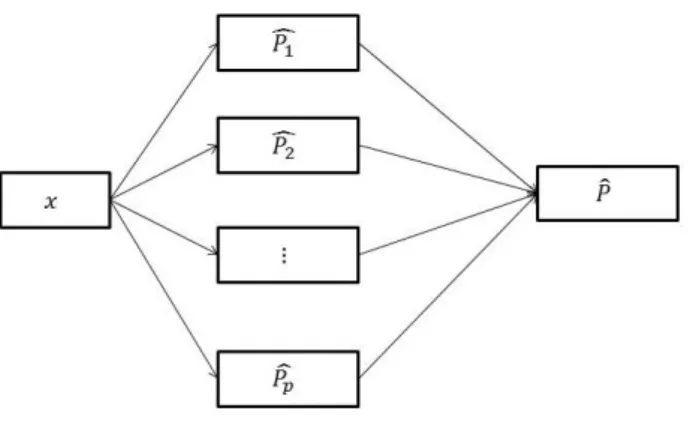
Figure 1: Computation structure of the option pricing by Monte Carlo method.
The above formula can also be expressed as:
∂P ∂x =
∂E(V(S))
∂x =E( ∂V(S)
∂x ).
The above integral can be estimated using Monte Carlo simulation, assumingpsimulations:
c
∂P ∂x =
1
p
p
∑
k=1
∂V(g(x, Zk))
∂x .
Note that random innovation Z is now broken down to p discrete vectors Zk, each vector
corresponding to a simulation path. So if the simulation consists ofqtime steps thenZk∈Rq.
Correspondingly, the Monte Carlo estimator for the price is:
ˆ
P = 1
p
p
∑
k=1
V(g(x, Zk))≡
1
p
p
∑
k=1 ˆ
Pk,
We illustrate the structure of the computation below in Figure 1, where ˆPk represents
sim-ulation path corresponding to innovation Zk ∈Rq. Due to the characteristics of the Monte
Carlo method, the derivatives of the price ˆP can be estimated pathwise. Thus, our general structure idea is simplified.
It is easy to see that structure (2.1) applies to the evaluation of f(x) ≡ Pˆ(x), where
vectorykhas no dependence on vectoryj,j < kin this case. Summarizing, (2.1) reduces to:
Solve for y1 : T1(x)−y1 = 0 Solve for y2 : T2(x)−y2 = 0 ..
.
Solve for yp : Tp(x)−yp = 0
Solve for z: ¯f(x, y1, y2,· · ·, yp)−z= 0
(4.15)
where Tk(x) ≡ Pˆk, k = 1,· · ·p. This special case of the structured form (2.1), where the
transition functionsTkdepend only on the control variablesx, and not on any previous state
vector yj,j < k, is known as a generalized partially separable function. Many functions in
science and engineering exhibit partial separability. When ¯f(x, y1,· · ·, yp) is a simple
aver-aging computation, i.e., ¯f(x, y1,· · ·, yp) = 1p
∑p
k=1yk then we call this a partially separable function. Specifically, the corresponding extended Jacobian matrixJE (2.2) can be written
as
JE =
J1
x −I
Jx2 −I
..
. . ..
Jxp ... −I
0 ∇f¯yT1 · · · ∇f¯yTp
.
The gradient is given by (2.3), which in generalized partially separable case reduces to:
∇fT(x) =
p
∑
i=1
∇f¯T yi∇J
i x.
The Algorithm for Structured Gradient can be reduced as follows.
Algorithm 2 Algorithm for Compute-GPS-Gradient (C-GPS-G)
1. Evaluateyi =Ti(x), i= 1,· · ·, p.
2. Evaluate and differentiate f¯(y1,· · ·, yp) using reverse-mode AD to get wi =∇f¯yi, i=
1,· · ·, p.
3. Compute by reverse-mode AD: vTi = wiTJi, where Ji is the Jacobian of Ti(x), i =
1,· · ·, p. Set∇f(x)←∑pi=1vi.
So Algorithm for Compute-GPS-Gradient calculates the gradient of a (generalized) partially separable function in time proportional toω(f) and spaceσsatisfyingσ ∼max{ω( ¯f), ω(Ti(x)), i=
ω( ¯f). So for large p, Algorithm for Compute-GPS-Gradient will require significantly less memory. Specifically, for largep
ω(f)≫max{ω( ¯f), ω(Ti(x)), i= 1,· · ·, p}.
Note that it is not necessary to follow any particular order over the indicesi,i= 1,· · ·, pwhen updating ∇f. When ¯f(x, y1,· · ·, yp) ≡ 1p
∑p
k=1yk further simplifications to the gradient
algorithm can be made. Specifically, in this case it is know that ∇f¯yi = 1/pand so steps 1,2
inCompute-GPS-Gradientare not needed and so the simplified gradient algorithm becomes:
Algorithm 3 Algorithm for Compute-PS-Gradient (C-PS-G)
1. Let∇f ←0
2. for k= 1 :p
3. Compute by reverse-mode AD applied to function Ti with “matrix” 1, vTi = 1·Jxi 4. ∇f ← ∇f +vi/p.
Note that if the memory requirement for the reverse mode in Step 3 is large, our general structure idea can be used to compute the vector viT forTi as well so that the memory can
be saved significantly.
There are a number of problem-dependent ways in which the basic gradient computation methods, given above in Algorithm for C-PS-G and C-GPS-G can be further improved in speed. First there is pruning. Pruning is based on the following observation: payoffs of options are usually of the following form:
[ST −K]+ or [K−ST]+.
HereST is the value of the underlying asset at timeT andKis the strike price. As discussed
in the previous section, the path-wise derivative estimator has the form:
1
p
p
∑
k=1
∂V(g(x, Zk))
∂x 1{STk>K}
where 1{STk>K} is the indicator function that flags if the value of the underlying asset is
bigger than K at timeT. Due to this indicator function, ∂V(g(x,Zk))
∂x 1{STk>K} will be zero
regardless of the value of ∂V(g(x,Zk))
∂x ifST < K. This property implies that there is no need
to generate the value of ∂V(g(x,Zk))
∂x in the case of ST < K. We need only set the value of ∂V(g(x,Zk))
∂x 1{STk>K} to zero. For reverse-mode AD, it is natural to do this since before
to generate the value of ∂V(g(x,Zk)) ∂x .
Due to this additional structure, reverse-mode AD can save significant calculation time compared with the forward mode. This comparison will be especially sharp for options that are deep out-of-the-money. Moreover, due to the put-call parity, we can further employ this property for options that are deep in-the-money. Put-call parity is the following relationship:
Ct+Ke−r(T−t) =Pt+St.
Here Ct and Pt are the prices of call and put options at time t. K is the strike price andr
is the continuous interest rate.
To illustrate, consider the computation of vega. If we differentiate the above equation on both sides with respect toσ, we have
∂Ct
∂σ = ∂Pt
∂σ,
since ∂(Ke∂σ−rt) = ∂St
∂σ = 0. Suppose we want to evaluate vega for a call option that is deep
in-the-money with reverse-mode AD. The indicator function1{S
Tk>K} has a significant
prob-ability of being non-zero. This means that we would have to perform the reverse sweep most of the time. However, due to (3.9), we can evaluate the vega of the put option and then induce vega for the call option. The put option will be deep out-of-the-money and reverse sweep can be omitted most of the time.
By rearranging the order of forward sweep and reverse sweep, this structure further al-lows us to save space for the reverse-mode AD. For the forward sweep to determine the payoff of the option, we only save the random numbers generating the path of the price and do not store all the other intermediate variables. Then only the random numbers with options in-the-money will be kept. After going through all the random paths, we perform an additional forward sweep for the paths that are in-the-money to generate the interme-diate variables again and then perform the reverse sweep to get the path-wise estimators for the Greeks. For options that are out-of-the-money, the additional backward sweep will only represent marginal additional computation but will produce considerable space savings. For options that are deep in-the-money, we can utilize the put-call parity mentioned in the previous paragraph to avoid much needless calculation, and save space at the same time.
5
Numerical Experiments
Maturity\ Strike 85% 90% 95% 100% 105% 110% 115% 120% 0.695 101.9 76.26 52.76 32.75 16.47 6.02 1.93 0.62
1 108 83.6 61.55 41.57 25.41 12.75 5.5 2.13 1.5 117.2 94.37 73.14 53.97 37.33 23.68 14.3 7.65
Table 1: S&P index European call option prices on October 1995 with strike price in the percentage of spot price.
Three typical experiments are considered in this section, the volatility inverse problem with and without smoothness term and Greeks for an interest rate derivative priced by the Li-bor market model. Note that the sparsity of the function Ti itself is not considered in our
experiments. A tape is used in the reverse-mode AD to record all intermediate variables in the function evaluation and gradient computation. In our experiments, the available fast memory is set to 500 MB for the reverse-mode AD, similar to the setting in ADOLC [2]. The purpose for this limit is to avoid affecting the performance of other applications on the machine during running the reverse-mode since it may use up all available fast memory as the tape grows. In other words, if the memory usage for the reverse-mode computation is more than 500 MB, only a chunk of the tape will be kept in memory while the rest will be written onto the hard drive. In the experiments, we use Matlab command matfile to read from and write to the hard drive. The times for accessing the hard drive depends on the times of total used memory and memory limit in the reverse sweep.
a. Local volatility surface construction
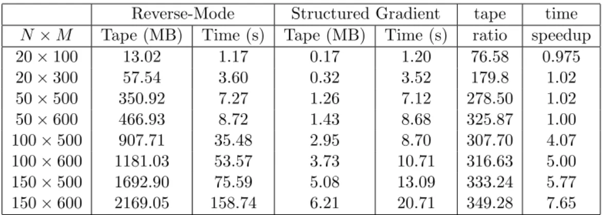
In this example, we assume that a set of European option prices of an underlying asset is given, then we try to calibrate the volatility surface σ(S, t) based on the PDE model (3.12) via the Crank-Nicholson finite difference method. Here we adapt S&P 500 market option price data for S&P 500 index options on October 1995 in Table 1. This data is also used in [3, 13, 14]. On this day, the S&P500 index value S0 = $590, interest rate r = 6% and dividend rate q = 2.62%. Then, the option prices are list in Table 1. Thus, we set the direct grid for (3.12) as [0.8S0, 1.2S0]×[0, T]. Table 2 records the memory and realized computational times of the gradient computation (3.7) based on the direct reverse-mode and structure gradient idea with various N ×M. The results in Table 2 show that the structure gradient computation saves the memory requirement (i.e., the length of whole tape) significantly. When the memory requirement of the direct reverse-mode is under the fast memory limit, the realized computational times for both methods are close. However, the direct reverse-mode takes much more computational times than the structure gradient method when running out of the fast memory.
b. Local volatility surface construction with smoothness term
Reverse-Mode Structured Gradient tape time
N ×M Tape (MB) Time (s) Tape (MB) Time (s) ratio speedup 20×100 13.02 1.17 0.17 1.20 76.58 0.975 20×300 57.54 3.60 0.32 3.52 179.8 1.02 50×500 350.92 7.27 1.26 7.12 278.50 1.02 50×600 466.93 8.72 1.43 8.68 325.87 1.00 100×500 907.71 35.48 2.95 8.70 307.70 4.07 100×600 1181.03 53.57 3.73 10.71 316.63 5.00 150×500 1692.90 75.59 5.08 13.09 333.24 5.77 150×600 2169.05 158.74 6.21 20.71 349.28 7.65
Table 2: Length of tape and running times of the gradient computation based on the struc-ture and direct reverse-mode AD for the local volatility surface construction problem.
introduce the cubic spline and the smoothness term into the objective function. The cubic spline idea is introduced to emphasize smoothness in the solution. Rather than estimating the volatility surface σ(S, t) at each Si and tj in the whole discritization grid, we only
esti-mate a few spline knots value ofσ(S, t) while other grid values are estimated as a function of cubic spline of these knots. An advantage of this idea is to reduce the number of variables,
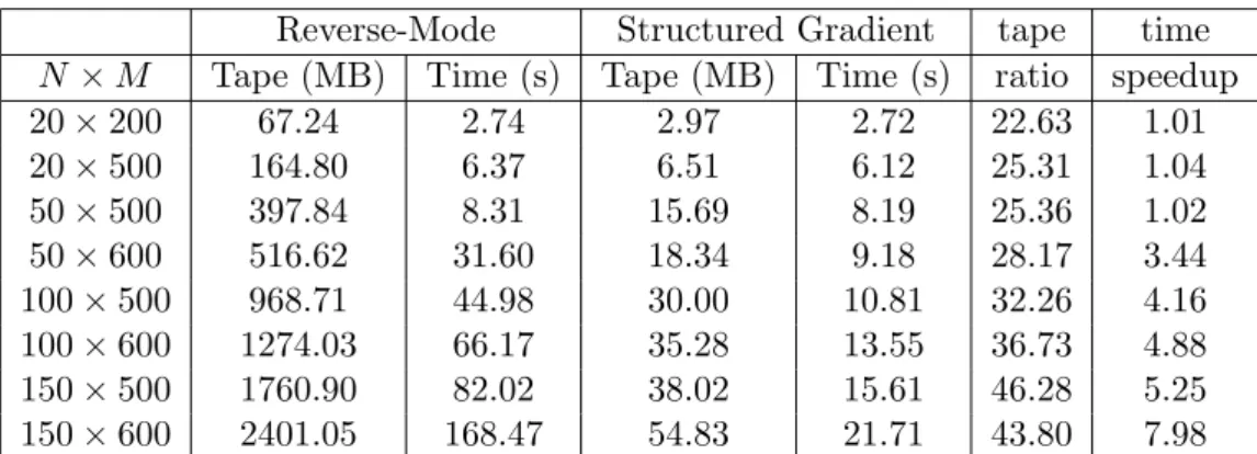
σ(S, t), fromN×M to a small fixed number. Determining the number of spline knots itself is tricky. Thus, in order to further balance the error and the smoothness of the surface, we introduce a smoothness term in the objective function in (3.9). Table 3 records the memory and realized computational times with the number of spline knots equals 10×10 and various
N×M. Table 4 records the memory and realized computational times with various numbers of spline knots andN ×M = 100×500. In Table 3, similar results are given as in Table 2. The structured gradient computation saves memory and realized computing time, especially when fast memory runs out. From Table 4, it demonstrates that as the number of spline knots increases, the memory and computational time of the structured gradient computation increase very slowly while the direct reverse-mode increases dynamically. The reason for this dynamic increase is due to the number of access to the virtual memory on hard drive. For the 30×30 case, the memory requirement is about 983 MB, so it only needs to access the virtual memory once while it requires to access the virtual memory twice in the 50×50 case. Thus, it leads a dynamic increase in the computational time.
c. Interest rate derivatives priced by Libor market model
mea-Reverse-Mode Structured Gradient tape time
N ×M Tape (MB) Time (s) Tape (MB) Time (s) ratio speedup 20×200 67.24 2.74 2.97 2.72 22.63 1.01 20×500 164.80 6.37 6.51 6.12 25.31 1.04 50×500 397.84 8.31 15.69 8.19 25.36 1.02 50×600 516.62 31.60 18.34 9.18 28.17 3.44 100×500 968.71 44.98 30.00 10.81 32.26 4.16 100×600 1274.03 66.17 35.28 13.55 36.73 4.88 150×500 1760.90 82.02 38.02 15.61 46.28 5.25 150×600 2401.05 168.47 54.83 21.71 43.80 7.98
Table 3: Length of tape and running times of the gradient computation based on the struc-ture and direct reverse-mode AD for the spline local volatility surface construction problem with smoothness term on various number of grids.
Reverse-Mode Structured Gradient tape time
nx×ny Tape (MB) Time (s) Tape (MB) Time (s) ratio speedup 10×10 968.32 32.86 30.86 6.88 31.95 4.78 20×20 975.27 31.41 33.41 6.31 29.19 4.97 30×30 983.25 32.04 36.91 6.33 26.92 5.02 50×50 1008.81 39.25 47.83 6.74 21.09 5.82 70×70 1045.12 42.72 55.27 6.79 18.92 6.28
surement, the j-th point on the term structure of interest rate has the following dynamic:
dLj(t) =−Lj(t)
∑N
k=j+1
αkLk(t)
1 +αkLk(t)
σj(t)σk(t)ρjk
dt+Lj(t)σj(t)dWjN(t), (5.16)
whereLj(t) andLk(t) are the values of thej-th andk-th interest rates of the term structure
at time t,dLj(t) is the instantaneous increment of the j-th interest rate at time t, αk is a
constant about maturity, σj(t) andσk(t) are the volatility of the j-th andk-th interest rates
and ρjk is the correlation between the j-th andk-th interest rates.
The above dynamics demonstrate that the instantaneous increment of the j-th point on the term structure only depends on the values and volatilities of the points beyond cur-rent point on the term structure. We denote L(t) = [L1(t), L2(t),· · ·, LN(t)] and dL(t) =
[dL1(t), dL2(t),· · ·, dLN(t)] at timet, then the above dynamic can be written in a function
form
dL(t)≡f(L(t), σ(t)|dWN(t)).
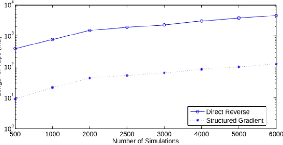
It is easy to show that the Jacobian matrices, ∂L∂f(t) and ∂σ∂f(t) are upper triangular. Therefore, based on the special structures of the Jacobian matrices and the structure idea, the sensitivity delta of a swaption under LMM can be computed efficiently. In this experiment, we consider a ten year swaption with quarterly payments and it expires in five years. The simulation step is the same as payment period so there are twenty simulation steps. Figure 2 and Figure 3 illustrate the length of tape and the realized CPU times for computing the price of the swaption and corresponding Greeks based on the direct reverse-mode and structured gradient technique. Similar to results of the other two examples in this section, the structured gradient idea can save the required space and realized CPU times dynamically, especially when the number of simulations is large.
6
Conclusions
Automatic differentiation is a practical field of computational mathematics of growing in-terest across many industries, including finance. Use of reverse-mode AD is particularly interesting since it allows for the computation of gradients in the same time required to eval-uate the objective function itself - there is no analogy in finite differencing (where the usual finite-difference approach takes time proportional to the number of variables multiplied by the time to evaluate the objective function). Finite-differencing time can easily dominate the overall computing time.
500 1000 2000 2500 3000 4000 5000 6000 100
101 102 103 104
Number of Simulations
Length of Tape (MB)
Direct Reverse Structured Gradient
Figure 2: Length of tape of the gradient computation based on the structure and direct reverse-mode AD for Swaption based on Libor market model via Monte Carlo simulation.
500 1000 2000 2500 3000 4000 5000 6000 100
101 102 103
Number of Simulations
CPU Time (S)
Direct Reverse Structured Gradient
available RAM) and, in others, slower than expected due to use of secondary memory and non-localized memory references.
A general technique known as “checkpointing” has previously been proposed to reduce the storage required to implement reverse-mode AD [20, 21] in gradient computations. In this pa-per we have observed and illustrated that many complex functions arising in finance exhibit a natural “substitution structure”; if this structure is explicitly exposed in the presentation of the objective function, then checkpoint location, state variables to be saved at the check-points, and explicit and efficient gradient computing formulae are all readily available.
The finance examples we have used here to demonstrate this structural approach are important and broad examples, not narrow in any sense. Nevertheless they are examples -without question there are many other examples in computational finance amenable to this structured AD approach.
What about more general Jacobians and Hessian matrices? There has been considerable work on determining such derivative matrices for structured (and sparse) problems. Most of this work utilizes sparsity in some way - either explicit sparsity in the derivative matrices themselves [15, 12], or “hidden sparsity” that shows up below the surface in the structured form [30]. We note that the approach provided here for gradients does not utilize any “hid-den sparsity” and this allows for a simpler implementation. The extension of this idea in the case of general Jacobians, and Hessians is currently being explored by the authors.
Fast and accurate gradient computation is useful in optimization in general, and compu-tational finance specifically, in itself. For example determination of Greeks (say for hedging purposes) is an important gradient computation. In optimization while it can be advan-tageous to accurately compute Hessian matrices, there are many effective optimization ap-proaches built strictly on gradient evaluation. For example, quasi-Newton methods (eg., [18]) and nonlinear conjugate gradient methods [22] require first derivatives (and only first derivatives). In addition, a fast gradient code can be used to approximate the Hessian ma-trix by finite differences (usually a much better approach, numerically, than approximating the Hessian with double finite differences using the function code). If the Hessian matrix is sparse then the fast gradient approach illustrated here can be used to approximate the Hes-sian matrix, by difference the gradient, in compact space (as we have illustrated here) and in time proportional toχ(H)·ω(f), where χ(H) is the chromatic number of the adjacency graph of the Hessian matrix H, and ω(f) is the number of operations required to evaluate
f(x). For sparse problems oftenχ(H)≪n.
References
[1] Cayuga Research, ADMAT-2.0 User’s Guide, www.cayugaresearch.com, 2013.
[2] ADOLC package, https://projects.coin-or.org/ADOL-C, 2013.
[3] L.B.G., Andersen, and R. Brotherton-Ratcliffe, The equity option volatility smile: an implicit finite difference approach, J. Comput. Finance Vol.1, 1997, 5C37.
[4] M. Bartholomew-Biggs, S. Brown, B. Christianson and L. Dixon, Automatic differenti-ation of Algorithm, J. Comput. App. Math. Vol. 124, 171-190, 2000.
[5] L. Capriotti and S. Lee, Adjoint Credit Risk Management, to appear in Risk.
[6] L. Capriotti and M. Giles,Fast correlation Greeks by adjoint algorithmic differentiation, Risk, 79-83, 2010.
[7] L. Capriotti and M. Giles , Adjoint Greeks made easy, Risk, 96-102, September 2012.
[8] L. Capriotti, S. Lee and M. Peacock, Real time counterparty credit risk management in Monte Carlo, Risk Magazine, 2011.
[9] Z. Chen and P. Glasserman, Sensitivity estimates for portfolio credit derivatives using Monte Carlo, Finance and Stochastics, Vol.12, 2008, 507-540.
[10] Z. Chen and P. Glasserman, Fast pricing of basket default swaps, Operations Research Vol. 56, 2008, 286-303.
[11] T. F. Coleman, X. Xiong, and W. Xu, Using Directed Edge Separators to Increase Efficiency in the Determination of Jacobian Matrices via Automatic Differentiation, Recent Advances in Algorithmic Differentiation Lecture Notes in Computational Science and Engineering, Springer, 87, 2012, 209-219.
[12] T.F. Coleman and G.F. Jonsson,The efficient computation of structured gradients using automatic differentiation, SIAM J. Sci. Comput., Vol. 20, 1999, 1430–1437.
[13] T. F. Coleman, Y. Li and A. Verma,Reconstructing the Unknown Local Volatility Func-tion, J. Comput. Finan., Vol. 2, 77-102, 1999.
[14] T. F. Coleman, Y. Li and C. Wang,Stable local volatility function calibration using spline kernel, Comput. Optim. Appl., DOI 10.1007/s10589-013-9543-x, 2013.
[15] T.F.Coleman and A.Verma,The efficient computation of sparse Jacobian matrices using automatic differentiation, SIAM J. Sci. Comput. Vol. 19, 1998, 1210–1233.
[17] C.H. Cristian, Adjoints and Automatic (Algorithmic) Differentiation in Computational Finance, Available at SSRN 1828503, 2011.
[18] J.E. Dennis and R.B. Schnabel, Numerical Methods for Unconstrained Optimization and Nonlinear Equations, SIAM, Philadelphia, PA, 1996.
[19] M. Giles and P. Glasserman, Computation methods: Smoking adjoints: fast Monte Carlo Greeks, Risk, Vol.19, 2006, 88-92.
[20] A.Griewank and A. Walther, Algorithm 799: Revolve: An Implementation of Check-pointing for the Reverse or Adjoint Mode of Computational Differentiatio, ACM Trans. on Math. Soft.,Vol.2, 19-45, 2000.
[21] A. Griewank and A. Walther, Evaluating Derivatives : Principles, and Techniques of Algorithmic Differentiation2nd Ed., SIAM, Philadelphia, PA, 2005.
[22] W. W. Hager and H. Zhang,A survey of nonlinear conjugate gradient methods , Pacific journal of Optimization, Vol.2, 2006, 35-58.
[23] L. Hascoet and M. Araya-polo,Enabling user-driven checkpointing strategies in reverse-mode automatic differentiation,European Conference on Computational Fluid Dynam-ics, P. Wesseling, E. O˜nate and J. P´eriaux (Eds), 1-19, 2006.
[24] M. Leclerc, Q. Liang and I. Schneider,Interest rates-Fast Monte Carlo Bermudan Greeks, Risk, Vol.22, 2009, 84-87.
[25] M. Joshi and C. Yang, Fast Delta computations in the swap-rate market model, J. of Economic Dynamics and Control, Vol.35, 2011, 764-775.
[26] M. Joshi and C. Yang, Efficient Greek estimation in generic swap-rate market models, Algorithmic Finance, Vol.1, 2011, 17-33.
[27] M. Joshi and C. Yang,Fast and accurate pricing and hedging of long-dated CMS spread options, International Journal of Theoretical and Applied Finance, Vol.13, 2010, 839-865.
[28] C. Kaebe, J. H. Maruhn, and E. W. Sachs, Adjoint based Monte Carlo calibration of financial market models, J. of Finance and Stochastics, Vol.13, 2009, 351 379.
[29] U. Naumann,Reducing the Memory Requirement in Reverse Mode Automatic Differen-tiation by Solving TBR Flow Equations, Lecture Notes in Computer Science, Vol. 2330, 1039-1048, 2002.
[30] A. Walther, Computing Sparse Hessians with Automatic Differentiation, ACM Trans. Maths. Soft., Vol. 34, 2008, 1-15.