UTILIZING MULTILEVEL EVENT HISTORY ANALYSIS TO MODEL TEMPORAL CHARACTERISTICS OF FRIENDSHIPS UNFOLDING IN DISCRETE-TIME SOCIAL
NETWORKS
Danielle O. Dean
A dissertation submitted to the faculty of the University of North Carolina at Chapel Hill in partial fulfillment of the requirements for the degree of Doctor of Philosophy in the
Department of Psychology (Quantitative).
Chapel Hill 2015
Approved by:
Daniel Bauer
Kathleen Gates
David Thissen
Mitch Prinstein
ABSTRACT
A social network perspective can bring important insight into the processes that shape
human behavior. Longitudinal social network data, measuring relations between individuals
over time, has become increasingly common – as have the methods available to analyze such
data. Adding to these methods, a modeling framework utilizing discrete-time multilevel survival
analysis is proposed in this dissertation to answer questions about temporal characteristics of
friendships, such as the processes leading to friendship dissolution or how long it takes an
individual to reciprocate a friendship. While the modeling framework is introduced in terms of
understanding friendships, it can be used to understand micro-level dynamics of a social network
more generally, such as the duration of reciprocated ties (or undirected relations) and the timing
of reciprocal actions. Similar to the model proposed by de Nooy (2011), these models can be fit
with standard generalized linear mixed model software, after transforming the data from a
network representation to a pair-period dataset. Two main models are introduced as part of the
framework, and a simulation study and empirical example are proposed for each. The first
empirical example concerns friendship duration in high school students and the second concerns
the timing of reciprocal “following” actions on the social network site Twitter. Advantages of
the modeling framework are highlighted, and potential limitations and future directions are Danielle O. Dean: Utilizing multilevel event history analysis to model temporal characteristics
TABLE OF CONTENTS
LIST OF TABLES ... vi
LIST OF FIGURES ... viii
LIST OF ABBREVIATIONS ... x
Chapter 1: Introduction ... 1
Goals ... 2
Models for Network Data... 3
Event History Analysis ... 5
Event History Analysis for Social Networks ... 8
Proposed Modeling Framework ... 10
Chapter 2: Friendship Duration (FD) Model ... 13
Simulation Study ... 18
Results ... 23
Application to High School Network Data ... 35
Results ... 39
Conclusion ... 42
Chapter 3: Reciprocal Timing (RT) Model ... 43
Indistinguishable Nominator and Reciprocator ... 47
Data Augmentation Approach (AIP approach) ... 49
Simulation Study ... 53
Results ... 55
Application to Reciprocity on Twitter ... 63
Results ... 67
Conclusion ... 71
Chapter 4: Conclusion ... 74
APPENDIX A: Tables ... 80
A.1: FD MODEL APPLICATION... 80
A.2: RT MODEL WITH KNOWN IDENTIFIERS ... 81
A.3: RT MODEL – WMM APPROACH ... 89
A.4: RT MODEL – AIP APPROACH ... 93
APPENDIX B: FIGURES ... 97
LIST OF TABLES
Table 1: Construction of pair-period dataset. ... 15
Table 2: FD Model – Simulation conditions summary. ... 23
Table 3: FD Model Bias and Relative Bias of Parameter Estimates. ... 25
Table 4: FD Model Standard Error Recovery. ... 26
Table 5: FD Model Application – Fixed Effects. ... 40
Table 6: FD Model Application – Covariance Parameter Estimates. ... 40
Table 7: Construction of pair-period dataset, known nominator and reciprocator. ... 46
Table 8: Construction of pair-period dataset, weighted approach. ... 49
Table 9: RT Model – Simulation conditions summary. ... 54
Table 10: Predictors definition for RT model of Twitter data. ... 67
Table 11: RT Model Application – Fixed Effects. ... 68
Table 12: RT Model Application – Random Effects. ... 71
Table 13: MFQ Scale. ... 80
Table 14: RT Model with known identifiers – MCMC Simulation Fixed Effects Bias. ... 81
Table 15: RT Model with known identifiers – PQL Simulation Fixed Effects Bias. ... 82
Table 16: RT Model with known identifiers – MCMC Simulation Fixed Effect Standard Error Recovery. ... 83
Table 17: RT Model with known identifiers – PQL Simulation Fixed Effect Standard Error Recovery. ... 84
Table 19: RT Model with known identifiers – PQL Simulation Random Effects Bias. ... 86
Table 20: RT Model with known identifiers – MCMC Simulation Random Effect Standard Error Recovery. ... 87
Table 21: RT Model with known identifiers – PQL Simulation Random Effect Standard Error Recovery. ... 88
Table 22: RT Model with WMM approach – PQL Simulation Fixed Effects Bias. ... 89
Table 23: RT Model with WMM approach – PQL Simulation Fixed Effect Standard Error
Recovery. ... 90
Table 24: RT Model with WMM approach – PQL Simulation Random Effects Bias. ... 91
Table 25: RT Model with WMM approach – PQL Simulation Random Effect Standard Error Recovery. ... 92
Table 26: RT Model with AIP approach – PQL Simulation Fixed Effects Bias. ... 93
Table 27: RT Model with AIP approach – PQL Simulation Fixed Effect Standard Error
Recovery. ... 94
Table 28: RT Model with AIP approach – PQL Simulation Random Effects Bias. ... 95
Table 29: RT Model with AIP approach – PQL Simulation Random Effect Standard Error
LIST OF FIGURES
Figure 1: Example event history functions for reciprocating a friendship. ... 8
Figure 2: FD Model Nesting Diagram. ... 16
Figure 3: Links per Node Simulation Factor. ... 20
Figure 4: Hazard factor definition... 21
Figure 5: FD Model – Intercept Recovery, High Hazard Condition. ... 28
Figure 6: FD Model – Intercept Recovery, Low Hazard Condition. ... 29
Figure 7: FD Model – True Effect (Pair-level Covariate) Recovery. ... 31
Figure 8: FD Model – Low Random Effect Standard Deviation Recovery. ... 33
Figure 9: FD Model – High Random Effect Standard Deviation Recovery. ... 34
Figure 10: Sample estimated functions for high school friendship data. ... 37
Figure 11: Depression. ... 38
Figure 12: Friendship Dissolution by Gender. ... 41
Figure 13: RT Model Nesting Diagram. ... 44
Figure 14: Dyad ties over time when studying reciprocation. ... 45
Figure 15: RT Model – Intercept Recovery, High Hazard. ... 56
Figure 16: RT Model – Intercept Recovery, Low Hazard. ... 57
Figure 17: RT Model – True Effect Recovery. ... 58
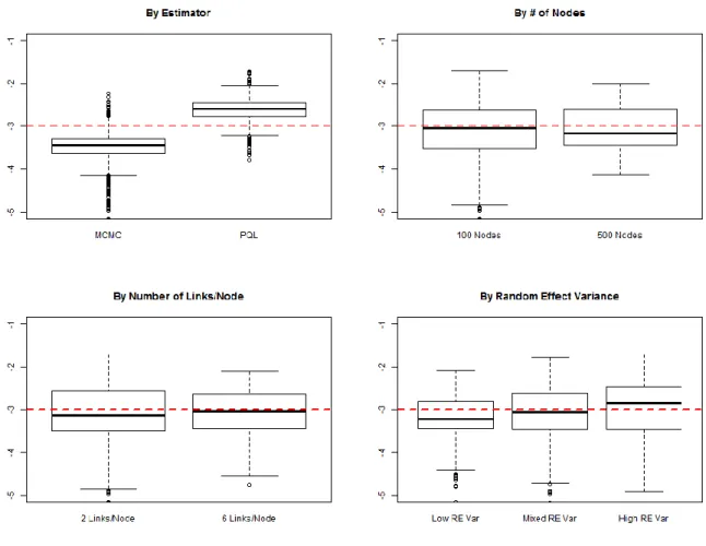
Figure 18: Intercept bias comparison of different approaches. ... 60
Figure 20: Reciprocator random effect bias comparison of different approaches. ... 63
Figure 21: Effects of the Nominator’s Number of Friends and Followers. ... 70
Figure 22: Effect of Protected Account of the Nominator. ... 71
Figure 23: RT Model – Standard Deviation of Nominators Random Effect Recovery, Low
Nominator Random Effect. ... 97
Figure 24: RT Model – Standard Deviation of Nominators Random Effect Recovery, High Nominator Random Effect. ... 98
Figure 25: RT Model – Standard Deviation of Reciprocators Random Effect Recovery, Low Reciprocator Random Effect... 99
Figure 26: RT Model – Standard Deviation of Reciprocators Random Effect Recovery, High Reciprocator Random Effect... 100
Figure 27: Gathering data from Twitter. ... 101
LIST OF ABBREVIATIONS
AIP Alternating Imputation Posterior estimation
FD Friendship Duration
GLMM Generalized Linear Mixed Model
ICC Intraclass correlation
MFQ Mood & Feelings Questionnaire
MCMC Markov Chain Monte Carlo
PQL Penalized quasi-likelihood
RT Reciprocal Timing
Chapter 1: Introduction
In recent years psychologists and other social scientists have become increasingly
interested in analyzing network data, recognizing that social networks play a key role in people’s
lives (Borgatti, Mehra, Brass, & Labianca, 2009; Wasserman & Faust, 1994; Snijders, 2005a).
For example, attributes of adolescent peer networks are important predictors of an individual’s
substance use (Ennett, et al., 2006) and socialization and social selection within networks play
important roles in shaping adolescents’ religious beliefs and behaviors (Cheadle & Schwadel,
2012). The rapid rise and influence of virtual social networks such as Facebook and Twitter
have also highlighted the existence of network structures and have become a focus of research as
well as a vehicle for studying network effects for many researchers (Cha, Haddadi, Benevenuto,
& Gummadi, 2010; Romero & Kleinberg, 2010).
Although a variety of models have been developed to identify and study the basic
structure of social networks, many fundamental questions remain stubbornly difficult to address
using current analysis approaches. Example questions may include those surrounding friendship
dissolution such as, “What are the processes leading to a friendship ending and what’s the role of
the individuals’ depression in this process?” as well as “How long does a typical friendship last
and does this differ between girls and boys?” Other example questions may surround reciprocal
tendencies, such as “Do some individuals reciprocate the actions of others more quickly than
other individuals?” as well as “Do people reciprocate actions more quickly if they are similar in
One common aspect of all of these questions is that they share a concern with dyadic
bonds within a network (e.g., specific friendships) rather than a concern with the global network
structure. Another is that they focus on understanding the processes leading to – as well as
timing of – an event occurring between two individuals, such as friendship formation or
dissolution. The overarching aim of this dissertation is to provide a modeling framework for
addressing such questions.
Goals
The first goal of this dissertation is to propose the use of multilevel event history models
to understand the processes leading to an event occurring between two individuals embedded
within a social network. This proposed modeling framework enables analysis of how long
friendships last and whether and when people reciprocate actions as well as the processes leading
to these events, for example. The second goal is to test the use of these models under
representative conditions that would be found in social network data. The last goal is to
demonstrate the application of the modeling framework through two empirical analyses.
To accomplish the goals outlined above, I first provide some background and preliminary
developments for the models to be investigated in this dissertation in the remainder of this
chapter. First, I describe shortcomings in extant modeling approaches for addressing questions
concerning event occurrence among dyads embedded in the network. Second, I discuss the use
of event history models for social network data, leading to the general modeling framework to be
investigated within this dissertation: a survival analysis approach that takes account of the
special features (e.g., dependencies) present within network data. Subsequent chapters elaborate
Models for Network Data
Statistical models with a social network perspective are often concerned with modeling
the processes leading to a network’s structure, known as social selection processes (Daraganova
& Robins, 2013; Anderson, Wasserman, & Crouch, 1999). In other words, the entire network is
often the outcome of interest. For example, network structure – specifically the formation of ties
between nodes such as friendship nominations between peers – can be modeled using
exponential random graph models (ERGMs), commonly referred to as p* models (Wasserman &
Robins, 2005; Frank & Strauss, 1986). ERGMs are built on the idea that social networks are
stochastic and that the patterns evident within a given network can be seen as evidence of
specific local processes, such as reciprocity, transitivity, and homophily1 (Wasserman &
Pattison, 1996). In addition to these social selection models, models of social influence are also
common; these models aim to understand how a network’s structure may constrain an
individual’s behavior (Daraganova & Robins, 2013). This dissertation focuses only on models
for social selection processes, both for tie formation and tie dissolution, rather than on models for
social influence.
Importantly, social network analysis provides a formal framework for testing ideas about
the structure of relationships and an alternative to the assumption that individuals are
independent (Wasserman & Faust, 1994). Multilevel models have a strong relationship to social
network data due to their ability to account for the non-independence of individuals (Snijders &
Bosker, 2012; Goldstein, 2011; Raudenbush & Bryk, 2002). In fact, multilevel models – also
referred to as random effect models – have been applied to network data for several purposes in
the past. The “p2” model for example allows the incorporation of nodal and dyadic attributes
into a model of network structure for binary network data, utilizing random effects to represent
the remaining variability in the actor level structural parameters (van Duijn, Snijders, & Zijlstra,
2004; Holland & Leinhardt, 1981). Multilevel models are also very useful as applied to
connections in personal “ego” networks (Snijders, Spreen, & Zwaagstra, 1995; van Duijn,
Snijders, & Zijlstra, 2004) and to understand directed dyadic data as in the Social Relations
Model which can be estimated with a cross-classified multilevel model (Snijders & Kenny,
1999).
In addition to social network models as applied to cross-sectional network data,
longitudinal social network models have become increasingly popular in recent years to
understand network evolution. Many of these models are based on the assumption that observed
networks are the result of a continuous-time Markov process (Snijders, 2005a). Longitudinal
network data generally enables researchers to better understand the dynamics leading to an
observed network at a point in time than cross-sectional data as one can condition on the first
observation of the network to better understand the subsequent changes. For example, the
actor-oriented model as implemented in the software program SIENA is a general and flexible
framework that allows the probabilities of relational changes to depend on the entire network
structure, with actors assumed to change their ties in order to optimize an objective function
(Snijders, 2005a). Alternatively, Hanneke, Fu, and Xing (2010) build directly on cross-sectional
ERGMs to model longitudinal network data with a model referred to as a Temporal ERGM
(TERGM), adding an exponential family function for the transition probability of a network from
While these models provide a framework from which to evaluate the processes leading to
the network’s structure, they are not structured to understand whether and when a specific type
of event occurs between individuals embedded within the network. They are thus also limited
with respect to answering questions regarding the processes leading to the event, such as those
questions listed at the start of this chapter.
Event History Analysis
In contrast to standard social selection network models, the proposed modeling
framework was developed to answer research questions about temporal characteristics of
friendships – whether and when an event occurs between individuals embedded within a network
– and is not a general purpose social selection model. The proposed modeling framework does
not aim to understand the processes leading to the entire network structure, but rather the
processes leading to the occurrence and timing of specific events between dyads within a
network through the use of multilevel event history analysis.
Event history analysis is at the core of the proposed framework as it is useful for
understanding both whether and when events occur (event history models are also known as
survival models, duration models, or failure-time models). In the social and behavioral sciences,
the timing of an event can often be considered to be a discrete variable as data is often collected
from a panel study or the year of an event is measured rather than the exact timing, as is the case
with the timing of the events in the empirical applications in this dissertation. This paper thus
focuses on discrete-time event history models, which can easily handle “tied” event times where
two or more people have the same event time (Singer & Willett, 1993; Freedman, Thomton,
continuous-time data were indeed available (Vermunt, 1997). Also important for the purposes
here, discrete-time methods extend to incorporate time-varying covariates and a multilevel
structure relatively easily (Steele, 2008; de Nooy, 2011).
To formalize discrete-time univariate event history analysis, let us assume for now that
the event under study is non-repeatable in that an individual may only experience the event
once.2 An example event within directed social network data could be the timing of reciprocity
between individuals from when the first individual within the pair initiates a relationship. Let the
random variable E denote the event time and t the discrete time point, with t = 1, 2, … T. Due to
censoring where the event time is not known for all pairs, the probability mass function ft of E
is not straightforward to compute. However, a function known as the hazard can be utilized
instead by building on the conditional nature of event occurrence. The hazard function is the
conditional probability of event occurrence at a certain point of time, given the event had not
occurred at earlier time periods (Singer & Willett, 2003). The hazard is thus the unique risk of
event occurrence at a given time period, for those eligible to experience the event:
( )
( | ) ( | t 1) .
( 1)
t
P E t
h P E t E t P E t E
P E t
(1)
The hazard of event occurrence is a conditional probability bounded between 0 and 1 and
can be modeled with a generalized linear model (GLM) (Hedeker, 2005; Agresti, Booth, Hobert,
& Caffo, 2000; Singer & Willett, 1993). With the unit of observation denoted i, a model with a
vector of predictors x and associated vector of fixed effectsβmay be written as:
'
~ it
t
t it
i i logit h
y Bernoulli h
x β
. (2)
For example, suppose we aim to predict whether an individual will reciprocate a friendship after
a friendship is initiated toward him or her (ignoring for now the dependencies of social network
data). Further, suppose that there is an effect of gender and time such that females are more
likely to reciprocate across all time periods and the hazard of reciprocating decreases over time.
This model can be written (with example regression weights):
0.25 0.5 female 0.5 time
~
it i
it it
it logit h
y Bernoulli h
. (3)
Through simple algebra, the hazard function can then be used to find the cumulative probability
of event occurrence, which may be more intuitive to interpret (Singer & Willett, 2003).3 The
equation above would result in a cumulative probability of 0.89 of reciprocating the friendship
by four time periods for a female and 0.77 for a male, for example, as visualized in Figure 1
below.
Event History Analysis for Social Networks
While event history analysis is commonly used in medical research, relatively few
applications exist of event history analysis to social network data and questions. Focusing on
models for social selection processes, applications are especially rare and nearly exclusively rely
on continuous-time measurement of the network (Krempel, 1990; Hu, Kaza, & Chen, 2009;
Kossinets & Watts, 2009; Butts, 2008). Others have focused on the propensity to be involved in
ties but not specific tie formations (Robinson & Smith-Lovin, 2001; Tsai, 2000; Kim & Higgins,
2007). However, the vast majority of applications involving event history analysis and network
data are social influence applications where network features are used as predictors in an event
history analysis of another outcome, such as understanding the impact of the composition of a
person’s network on their health (Adams, Madhavan, & Simon, 2002; Villingshoj, Ross,
Thomsen, & Johansen, 2006).
Figure 1: Example event history functions for reciprocating a friendship.
Event history models have rarely been used for social selection processes because of the
complexities arising from the dependencies in network data. Researchers applying event history
models to longitudinal social network data have largely either ignored dependencies (as was
done in the simple example in Figure 1), sampled pairs from an extremely large network in order
to obtain independent observations, or used a fixed effects approach by for example adding a
dummy intercept in the model for all persons except one (Krempel, 1990; Kossinets & Watts,
2009; Butts, 2008; Brandes, Lerner, & Snijders, 2009). Ignoring dependencies can result in
biased parameter estimates and standard errors, potentially leading to incorrect conclusions (Guo
& Zhao, 2000). Also, while a fixed effects approach does adjust for all unmeasured covariates at
the person-level, it is not parsimonious, nor does it allow for inference beyond the individuals
within the sample and makes it difficult to examine person-level predictors (Snijders, 2005b, p.
665).
Fortunately, multilevel event history analysis can provide a parsimonious framework for
accounting for dependencies inherent in social network data (Steele, 2011; Goldstein, 2011;
Rabe-Hesketh & Skrondal, 2012). These models allow examination of both individual and
dyad-level covariates simultaneously as well as time-varying network context effects and permit
inference to the population from which the sample is drawn (Raudenbush & Bryk, 2002). De
Nooy (2011) recently applied a multilevel event history model to model the dynamics of
longitudinal network data on the timing of book reviews, utilizing cross-classified random
effects to account for the individual tendencies of book authors and reviewers within the directed
social network. Predictors within this model could include attributes of the book authors, the
structure such as transitivity – the tendency for a “friend of a friend” to become a friend.4
Discrete-time multilevel event history models are part of the generalized linear mixed model
(GLMM) family and can thus be fit using software that fits GLMMs such as SAS, MLwiN, and
R (Tuerlinckx, Rijmen, Verbeke, & De Boeck, 2006).5
Proposed Modeling Framework
The proposed modeling framework builds upon the prior application of the multilevel
event history model for social network data by de Nooy (2011) to study more generally the
processes leading to the occurrence and timing of events for individuals embedded within a
network, expanded to include undirected networks and outcomes such as reciprocity and
dissolution. The proposed modeling framework is sensitive to the fact that processes leading to
the creation of a symmetric relationship from an asymmetric one may be very different from the
processes leading to a tie forming within the pair at all (Cheng, Romero, Meeder, & Kleinberg,
2011; Luo, Tang, Hopcroft, Fang, & Ding, 2013). Also intuitively, processes leading to
friendship dissolution could be very different from the processes leading to tie formation.
4 Network context covariates can be calculated by counting subnetworks created by the formation (or dissolution) of
the tie being modeled from links that precede this tie (Wasserman & Pattison, 1996). The time ordering of the network thus allows network effects beyond the dyad to be included in the model in a straightforward manner without the “circular dependencies” that prohibit their inclusion in cross-sectional models of networks (de Nooy, 2011; Wasserman & Robins, 2005). One approach to including network context is to limit the context considered to lines appearing in the previous time period through a retrospective sliding window approach (Moody, McFarland, & Bender-deMoll, 2005). Alternatively, a decay function may be used to weigh network context by the length of time passed.
5 A review of estimation options as well as estimation issues related to GLMMs is outside the scope of this
For example, suppose one was interested in the tendencies for individuals to reciprocate
friendships within a high school social network. A general purpose social selection model may
reveal the effect of gender on the likelihood of an edge forming between two individuals within a
network, controlling for the effect of reciprocity. For example, there could be a positive
reciprocity effect, revealing that individuals are more likely to consider an alter to be a friend if
the alter already considered them a friend; controlling for this effect, females may be more likely
to consider other individuals to be a friend than males. Individuals are assumed to have the same
underlying tendencies to reciprocate and the covariates are predicting tie formation generally
rather than reciprocity.6 In contrast, the proposed modeling framework allows one to study the
effect of gender on the actual outcome of interest – the likelihood of reciprocating. It allows
individuals to vary in their underlying tendencies to reciprocate and be the product of
reciprocation; the modeling framework also answers questions about the timing of reciprocity,
such as the median time to reciprocation, in a straightforward manner as it actually models the
risk of reciprocating over time for each dyad.
Within this broader framework, this dissertation develops two specific models of network
events as examples: one for friendship duration in undirected networks, and one for the timing of
reciprocity in directed networks. For ease of exposition, the models that are introduced are
mainly described as models for understanding friendship, as this is the research domain within
which the models are applied in the empirical applications. However, these specific models aim
6 This may be relaxed somewhat by including an interaction term between gender and reciprocity, to understand
to be examples within a general framework through which other outcomes could be analyzed,
such as the timing of friendship duration in a directed network (e.g. perceived friendship
duration) or different types of relationships other than friendship (e.g. organizational ties). When
the outcome of interest is the timing of events occurring between individuals embedded within a
network, the proposed modeling framework provides a more straightforward path than global
network models for analyzing the data and evaluating the hypotheses of interest.
In addition to answering specific research questions which are important in their own
right, the modeling framework discussed in this dissertation has an advantage of being easily
applied to networks without clearly defined bounds (e.g., changing node set, sample from larger
network) and can easily handle censored event times (e.g. missing ties). Also, model fitting of
sparse data that is a ubiquitous problem for social network data – due to most dyads being
unconnected versus connected – is mitigated as the focus remains on specific dyadic processes
rather than the entire network.
In the remaining chapters, I formalize this modeling approach as well as test and apply
the framework. Within Chapter 2, the model for friendship duration is developed and then
subsequently tested with a simulation study and applied to high school friendship nomination
data. Within Chapter 3, the model for the timing of reciprocity is developed, tested under a
simulation study similar to Chapter 2 and then the use of the model is demonstrated with an
application to user followings on the social network site Twitter. Chapter 4 concludes with
discussion of the strengths and limitations of the proposed framework and directions for future
Chapter 2: Friendship Duration (FD) Model
As described in Chapter 1, this dissertation proposes the use of multilevel event history
analysis to study the processes leading to an event occurring between individuals within a dyad
of a social network as well as the timing of that event. Toward that goal, the “Friendship
Duration” (FD) Model is developed in this chapter to answer questions about the length of
friendships and processes leading to friendship dissolution. This model development was
motivated by an aim to model the processes leading to high school friendship dissolutions,
specifically to understand the role of gender and depression in friendship dissolution, which is
examined in the empirical example later in this chapter.
For the purposes of this model, friendship can be defined to start when both individuals
nominate each other as a friend in a directed network or a friendship is recorded for a pair in an
undirected network.7 More generally, this proposed model is useful for understanding the
duration of reciprocated ties in a directed network, or the duration of a tie in an undirected
network. As the model is concerned with the duration of the dyadic relationship, the process
being studied is dissolution rather than selection (e.g. examining whether and when the
relationship ends rather than why the relationship began in the first place). In this chapter, I first
develop the modeling framework including a description of how to structure the data, followed
by a simulation study and an empirical application.
For this model, consider the event process to begin when the ties are mutually
reciprocated (or in the case of an undirected network, when the tie first appears). Let the
outcome y in this case be a binary indicator, equal to 0 for time periods during which the ties
remain mutual and 1 for the time period when the ties are no longer mutual. For simplicity here,
it is assumed that once the mutual ties are dissolved, the ties remain in this state, although it is
possible to extend the model for repeatable events.
Right censoring is very likely to occur in data measuring friendship dissolution events, as
some individuals will remain friends throughout the observation period.8 However, unlike most
event history analyses, left censoring may also occur relatively often depending on how the
network is sampled – as individuals may be friends before observation begins.9 If start times of
the friendships are known, these left censored event times may be incorporated by the
conditional likelihood approach as outlined by Guo (1993). Thus one potential solution, which
must be considered before sampling data, is to ask participants to recall when the friendship first
began in addition to asking about their current friendships. Alternatively, careful selection of the
observation period may allow one to define the friendship for specific time periods. For
example, when sampling a friendship network from the beginning of high school to the end of
high school, no left-censored data would exist if the event process under study is “how long do
high school friendships last,” as the event process is thus defined to begin at the start of high
school at the earliest irrespective of whether individuals were friends prior to high school; this is
8 Right censoring is when the event of interest does not occur during the time frame of the study (in the friendship
duration case, this occurs when a friendship does not end during the study period).
9 Left censoring occurs when the event process begins before the observation period. Unlike right censoring which
the approach proposed for the empirical example in this chapter. Other alternatives include
simply deleting left censored observations – although this risks a potential selection bias (Cain,
et al., 2011), or incorporating the left-censored observations through more sophisticated
techniques, such as imputing event times (Karvanen, Saarela, & Kuulasmaa, 2010), which are
not discussed in this paper.
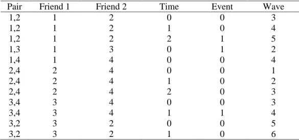
The dataset can be arranged in a “pair-period” structure where there is a row for each pair
by time combination during which the pair is eligible to experience friendship dissolution.
An example dataset for the model is given above in Table 1, where friend 1 and friend 2 are an
arbitrary numbering of individuals within the pair. A time of 0 signifies the first time period that
a friendship is eligible to dissolve after relationship formation and the outcome of interest is a
binary indicator y of whether or not the relationship ends at time t as discussed above. Thus,
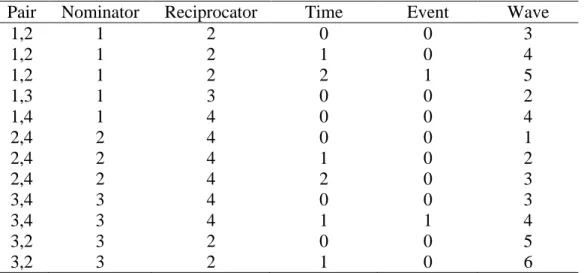
time in the model is dyad dependent and may represent different actual waves of data collection Table 1: Construction of pair-period dataset.
Time for a dyad begins when the relationship starts. “Time=0” is wave 3 for pair 1,2 but wave 2 for pair 1,3 for example.
Pair Friend 1 Friend 2 Time Event Wave
1,2 1 2 0 0 3
1,2 1 2 1 0 4
1,2 1 2 2 1 5
1,3 1 3 0 1 2
1,4 1 4 0 0 4
2,4 2 4 0 0 1
2,4 2 4 1 0 2
2,4 2 4 2 0 3
3,4 3 4 0 0 3
3,4 3 4 1 1 4
3,2 3 2 0 0 5
for different dyads. While the time scores need not be equidistant, the distance between the same
time periods for different pairs should be consistent.10
Often in multilevel models, the individuals or occasions within individuals are the lowest
level units of the analysis. However, the model described here is built in order to understand the
relationship’s duration, an outcome of the pair of individuals. We thus have pairs nested within
individuals (Goldstein, 2011, p. 260). Each pair is measured over time, creating a three level
structure. The model thus aims to understand whether and when the pair’s relationship ends,
accounting for the dependency that occurs from the fact a pair is nested within two individuals,
and these individuals contribute to multiple pairs.
This three level structure is visualized above in Figure 2, where the arrows represent the nesting
structure and to which higher level unit the lower level unit belongs (Rasbash & Browne, 2008).
Here, we have time nested within pairs which are then nested within individuals; for example,
10 However, the distance between the same time periods for different pairs is unlikely to be consistent in practice
unless data collection is specific to the timing within pairs, such as the data collection discussed in the empirical example in Chapter 3. For collection of data in waves where multiple pairs are examined around the same date, the time difference between waves should be consistent.
friendship between individuals 1 and 2 is recorded by “pair 1,2” over 3 time periods. While
pairs are made up of only two individuals, individuals may be involved in numerous friendship
pairs.
To formalize the model, let i and i’ be two individuals within a pair p, with the total
number of individuals I across pairs P. The hazard h of relationship duration, which represents
the risk or conditional probability of friendship dissolution given the friendship had not yet
dissolved, is modeled as a function of a vector of predictors x. These predictors could be time as
well as pair-level covariates, any of which may be allowed to vary over time (e.g. there could be
an effect of time, pair’s average depression, and an interaction between time and the pair’s
average depression). These predictors have an associated vector of fixed effects β. A random
effect u is added for each individual within the pair, making the model a multiple membership
multilevel model, in order to account for each individual’s underlying propensity for their
friendships to end (Goldstein, 2011; Rasbash & Browne, 2008). The random effects for all
individuals are assumed to be normally distributed with mean 0 and common variance 𝜎2. The
equations for the model are:
'
2 '
~
~ 0,
pt pt
p
i i
t pt
i
logit h u u
y Bernoulli h
u N
x β
. (4)
A high random effect would imply that an individual’s friendships are more likely to dissolve
different weights for different dyads to the random effects as each individual is assumed to be an
equal member of the dyad.11
Simulation Study
The goal of this simulation study is to test the practicality of the proposed models, under
a set of non-exhaustive but informative conditions. While multilevel event history models are by
no means unique, nor are multilevel models with multiple membership structures, these models
have yet to be tested together in the types of conditions that would arise in social network data
such as in the empirical example in the next section. The conditions are chosen to reflect
conditions that might be seen in practice, influenced in large part by preliminary analyses of the
data from the empirical applications in this chapter and Chapter 3. The main goals of the
simulation are to understand how the hazard rate and sample size – both in terms of the number
of individuals as well as the number of friendships per individual – influence the ability to
recover the fixed and random effects of the model. Additionally, the simulation study is
designed to reveal the influence of the estimation method chosen and the amount of dependence
in terms of the magnitude of the random effect variance.
The hazard function for this simulation study is constant in both the
population-generating model and fitted model (i.e. single intercept), and the number of time periods is held
constant at five to keep the scope of the simulation reasonable while focusing on more
interesting conditions. This number of time periods is chosen to be close to the empirical
examples, as the empirical example in this chapter has six time periods and the next chapter has
five time periods. One binary pair-specific true effect is included in all conditions to test
11 For example, a multiple membership model with school effects may have a weight which approximates the length
recovery, with a regression coefficient of 0.5 and a balanced mix of the two groups in the
population-generating model (e.g. in practice, this could be the effect of ‘same-gender’ versus
‘different-gender’ friendship pair with half of the pairs being one type versus another). One
pair-specific null effect is included to test false recovery with the predictor generated from the mean
of each individual’s predictor coming from a N(0,1) distribution (e.g. in practice, this could be
testing for an effect of the mean depression of the pair where no effects exists).
The number of individuals is varied at 100 or 500, reflecting reasonable sample sizes for
relatively small and relatively large network studies that are seen in psychology and related
disciplines (Schaefer, Light, Fabes, Hanish, & Martin, 2010; Ojanen, Sijtsema, & Rambaran,
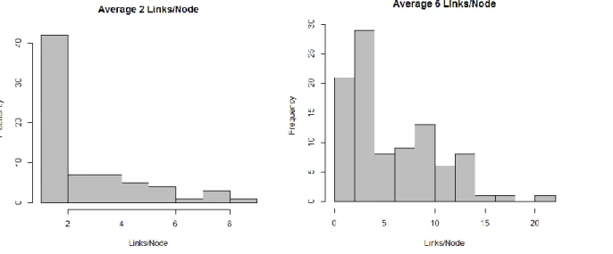
2013). The average number of links per node is varied at 2 and 6, again aiming to reflect a
reasonable low and high range of ties per node seen in practice (Dijkstra, Cillessen, & Borch,
2013; Ahn & Rodkin, 2014). Both of these types of conditions reflect similar values to what is
seen in the empirical applications in this chapter and the next chapter. Whether a link is ever to
occur between nodes is generated randomly until the average links per node in the network reach
this number; example distributions of the number of links per node are shown below in Figure 3.
The timing of the link dissolution is then simulated with the logit link function as specified in
The hazard risk is varied between “low” and “high” risk. Low risk is defined specifically
as an intercept within the logit function of -3, while high risk is an intercept of 0.05. These
values were chosen after preliminary analyses of the empirical applications in this and the next
chapter, as the “high” risk condition reflects a hazard function similar to what the friendship
duration data reveal in the next section of this chapter while the “low” risk condition reflects a
hazard function similar to the data analyzed in Chapter 3. These parameter choices result in the
hazard and survival functions plotted in Figure 4, when random effects are held at the population
average. High risk implies a probability of 0.51 of the event occurring at any time period for
pairs that are eligible to experience the event and only a 0.03 probability of the event not
occurring by the last time period, and low risk implies a conditional probability of 0.05 of the
event occurring at any time period, with a cumulative probability of 0.78 of the event not
occurring by the last time period.
Figure 3: Links per Node Simulation Factor.
Example distributions of links per node across individuals in two datasets, one with an average of two links per node and the other with an average of six links per node, with frequency
The random effect variance is varied at two levels ( 2
0.35,1.40 ). Previous research
has often found a downward bias in the estimated variance components when fitting GLMMs to
binary outcomes, the magnitude of which depends on a number of factors including the
estimation method as well on the size of the random effect variance which is why the random
effect variance is a factor in this simulation. With the two individuals in the pair p denoted i and
i’ respectively and an individual outside the pair denoted j, a latent variable conceptualization of
the binary response variable can be used such that the friendship dissolution event occurs if
* 0 p
y and does not otherwise, to define an intraclass correlation coefficient. With the FD
Model equation for the simulation then written as:
*
0 0.5 0 1 2 '
pt i i pt
y true nullu u , (5)
Figure 4: Hazard factor definition.
where 0denotes the intercept, true denotes the binary pair-level predictor that has a true effect,
null denotes the continuous pair-level predictor that has no effect,u1idenotes the latent variable
for the first individual and u2 'i denotes the latent variable for the second individual in the pair.
Assuming the errorptin Equation (5) follows a logistic distribution, an intraclass correlation
(ICC) can be defined for the multiple membership random effect as the correlation among latent
responses for the same person, conditional on the latent variable – underlying tendency to
dissolve friendships in the FD Model – of other individuals:
22 * *
' ' 2 2
2
3
, | i, j
ii ij
y
Corr y u u
. (6)
A random effect variance of 0.35 results in an ICC of 0.1 while a random effect variance
of 1.4 result in an ICC of 0.3. An ICC of 0.1 was chosen because preliminary analyses of the
empirical data in this chapter indicate an ICC close this value, without covariates in the model.
The higher ICC of 0.3 was chosen to test the model with a stronger dependence structure, but
low enough to reflect an ICC that might be seen in practice with similar network data, and is
close to the dependence seen in preliminary analyses of the empirical data in the next chapter.
The FD model is fit using pseudo-likelihood (PQL)12 through SAS GLIMMIX and using
MCMC techniques through the MCMCglmm package in R (Hadfield, 2010).13 Previous research
12 Although multiple membership and cross-classified models can be reformulated as multilevel models with nested
random effects (Rasbash & Browne, 2008), the approach requires the evaluation of integrals with high dimensions and is computationally burdensome. Numerical quadrature is not available as an option for multiple membership and cross-classified random effects using GLIMMIX, as “METHOD=QUAD” requires that model can be processed by subjects (SAS/STAT(R) 9.3 User's Guide, 2015).
13 Burn-in was set to 50,000 and the number of iterations at 100,000 with a thinning interval of 50 across all
has revealed that PQL is computationally efficient and is robust to starting values, performing
better with larger cluster sizes and smaller variance components, but has been found to result in
fixed and random effect estimates biased toward zero when modeling binary outcomes
(Rodríguez & Goldman, 1995; Rasbash & Goldstein, 1994; Bauer & Sterba, 2011). Maximum
likelihood approaches and MCMC perform best with a large number of clusters such that
asymptotic properties hold, as biased and highly variable estimates may result otherwise
(Tuerlinckx, Rijmen, Verbeke, & De Boeck, 2006; Bauer & Sterba, 2011).
In summary, the FD model is tested under 5 factors, together constituting 32 total
simulation conditions (2 x 2 x 2 x 2 x 2), and are summarized in Table 2 below. The models are
replicated 1000 times between the first four factors below and the same data is then used to fit
the model separately by PQL and MCMC.
Results
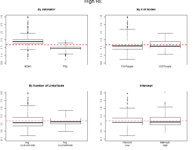
Performance is assessed by examining bias of the different parameter estimates (Table 3),
the standard deviation of the estimates compared to the standard error of the estimates (Table 4),
Type I error of the null effect, and power of the pair-level effect (Burton, Altman, Royston, &
Holder, 2006). Results are listed in Table 3 and Table 4 and then summarized after the tables by
Table 2: FD Model – Simulation conditions summary.
Number of Nodes
Links per
Node Hazard
Random Effect
Variance Estimation
100 2 low 0.35 PQL
examining specific conditions as well as aggregating across factors to determine how well the
: F D Mod el B ias and R elative B ia
s of Par
amete r E sti mate s. of t he parame te
rs across di
ff ere nt conditi ons ( factors i tal icize d ), w it h re lat ive bias gre
ater than 25% bolde
Ta ble 4 : F D Mod el S tanda rd E rr o r Re cov er y . Standar d de viat ion of parame ter e sti mate s c ompa re
d to me
an st andard e rr or ac ross r epli cati on (fac tors it ali cized) w it h condit ions b olded whe
n the ratio i
s of
f by m
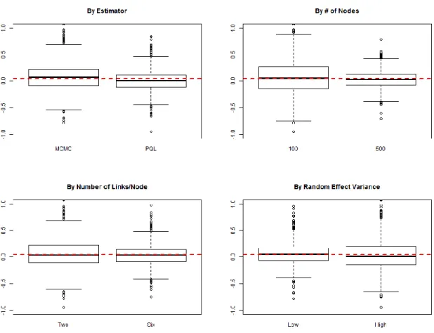
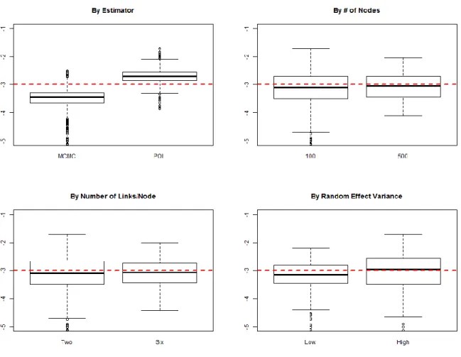
First examining recovery of the intercept (see Figure 5 and Figure 6 below), both MCMC
and PQL estimation methods have small absolute bias for the high hazard condition (when
β0=0.05)14 and larger absolute bias for the low hazard condition (when β0= -3) with MCMC
biased away from zero and PQL biased toward zero. While bias is relatively large in some cases
for the low hazard condition (as large as -0.79 with relative bias of 26%), this condition provides
a rather stringent test as the event occurs extremely rarely. For both the high and low intercept
conditions, MCMC estimation has larger variability across simulations than PQL (SD = 0.36
versus SD= 0.21). The worst estimation of the standard error of the estimates is for MCMC
estimation for 100 nodes and 2 links per node where the standard deviation of the estimates is
approximately twice the mean standard error of the estimates; however, the standard deviation of
the estimates and the mean standard error of the estimates is nearly identical for other conditions,
including all conditions with PQL estimation.
Aggregating across estimation methods, there is small or negligible bias in recovering the
intercept for other factors but a clear pattern in variability where the smaller number of nodes
and number of links per node result in greater variability in the estimates of the intercept; a larger
random effect variance also results in greater estimate variability. Examining results within
estimation method however, MCMC results in less average absolute bias when increasing from
100 to 500 nodes (0.39 versus 0.23) while the average absolute bias actually increases slightly
for PQL estimation when going from 100 to 500 nodes (0.16 versus 0.19). Both MCMC and
PQL result in less average absolute bias when increasing from 2 to 6 links per node.
Figure 5: FD Model – Intercept Recovery, High Hazard Condition.
Recovery of the true effect (pair-level covariate, β1=0.5 across all conditions) follows a
similar pattern, where MCMC estimation, as well as a smaller number of nodes, smaller average
links per node, and larger random effect variance result in greater variability in the estimates (see
Figure 7 below). The difference between 100 and 500 nodes makes the largest impact on the
power to detect a significant effect (on average 0.39 versus 0.86), although power is higher for
larger number of links per node, smaller random effect variance, and for the high intercept
condition. Similar to intercept recovery, MCMC estimation is biased away from zero while PQL Figure 6: FD Model – Intercept Recovery, Low Hazard Condition.
other factors. MCMC tends to result in larger relative bias than PQL (MCMC with average
relative bias of 18% versus PQL with average relative bias of 10%), with the difference
especially apparent for small sample sizes and with smaller links per node. MCMC estimation
again tends to result in less average absolute bias when increasing from 100 to 500 nodes (0.11
to 0.08) while the average bias for PQL between the two levels is similar on average (0.05 for
both levels). Despite these differences, PQL and MCMC result in similar power to detect a
significant effect, as well as the same pattern for power across the different factors. The
difference between a high and low intercept has little impact on bias and variability of recovering
Type I error of the null effect (pair-level covariate, β2=0 across all conditions) is as
expected, around 0.05 for α=0.05 for all conditions. There is negligible bias in the estimates Figure 7: FD Model – True Effect (Pair-level Covariate) Recovery.
reveals that MCMC estimation, a smaller number of nodes, smaller average links per node, and
larger random effect variance result in greater variability in the estimates, while the intercept
factor has little impact.
The standard deviation of the random effect (Figure 8) is consistently overestimated by
MCMC (average relative bias of 50%) and underestimated by PQL (average relative bias of
29%), for both low and high random effect conditions. The bias is quite severe with a smaller
number of nodes and links per node, especially for MCMC; however, we again see an
improvement in average absolute bias for MCMC when moving from 100 to 500 nodes (0.57
versus 0.39) but not for PQL (0.28 versus 0.31). The standard error of the random effect
variance also tends to be overestimated by MCMC, with the exception of small number of nodes
and links per node and low hazard when the standard error is largely underestimated (Table 4).
The bias in estimating the random effect variance is consistent with previous research on binary
outcome models with random effects, especially considering the number of links per node
(equivalent to the number of objects per cluster) is so small in such network data (Rodríguez &
Goldman, 2001; Rodríguez & Goldman, 1995). There is less variability in the estimates when
the number of nodes, as well as the number of links per node, is higher and also when the
Figure 8: FD Model – Low Random Effect Standard Deviation Recovery.
In summary, although recovery of the random effect tends to be poor, the model recovers
the fixed effect parameter estimates relatively well – especially when the number of nodes and
number of links per node is larger. Increasing the number of nodes has the largest impact on the
power to detect a significant pair-level effect and also improves the bias of MCMC estimation
results although not PQL estimation results. An increase in the number of links per node also
has a large influence on power, and improves results in terms of both bias and variability for both
MCMC and PQL estimation, as does a smaller random effect variance. Finally, PQL estimation
tends to have less variability in the conditions of this study than MCMC, and recovery tends to Figure 9: FD Model – High Random Effect Standard Deviation Recovery.
be better for the high intercept condition when the risk of event occurrence is higher. Now that
the model has been tested under relevant conditions to real social network data, we next apply
the FD Model to high school friendship duration data, the empirical example that motivated the
development of this model.
Application to High School Network Data
Friendship dissolution occurs when the relationship ceases to exist and is often
experienced with “considerable distress” (Baumeister & Leary, 1995, p. 503). Researchers have
found that friendship serves different purposes for men and woman; from as early as preschool to
adulthood, gender differences within friendships have been noted (Maccoby, 1990; Johnson &
Aries, 1983). Females have been found to develop closer and more intimate relationships in
general, and some researchers argue dissolution tends to be more significant for females as a
result (Jalma, 2008). While dissolution is an important phase of many relationships, most
research has focused solely on the mechanisms leading to friendship formation. Schaefer,
Kornienko, and Fox (2011), for example, found that depression homophily could be created in a
network through a withdrawal mechanism even in the absence of preference. However,
comparatively little research has analyzed the factors leading to friendship dissolution and that
research which has focused on dissolution has largely focused on romantic relationships
(Sprecher, 1988; Felmlee, Sprecher, & Bassin, 1990).
In this empirical example, the processes leading to high school friendship dissolutions
and the length of high school friendships are examined, especially in relation to the influence of
gender and depression. Students were recruited at the beginning of high school, in the fall of
collection began in February of ninth grade (in 2009), and collections took place at
approximately six-month intervals through the spring of their twelfth grade year, with seven
waves of data collection total.15
At each wave of data collection, students were given a current roster and allowed to
nominate an unlimited number of individuals that they considered to be their friends. A
friendship pair was considered to exist when both individuals within the pair nominated each
other as friends. A total of 814 friendship pairs existed for at least two time periods of which
194 were male friendship pairs, 391 were female friendship pairs, and 229 were mixed gender
friendship pairs. The friendship pairs were drawn from a total of 339 individuals (42% male).
For each pair, time was coded to indicate when the friendship began (rather than the wave of data
collection), and a binary indicator of friendship ending was created if either or both of the
individuals failed to nominate the other individual within the pair as a friend. Friendship pairs
were included for all time periods when both individuals within the pair provided nominations
until the first friendship dissolution or censoring occurred.
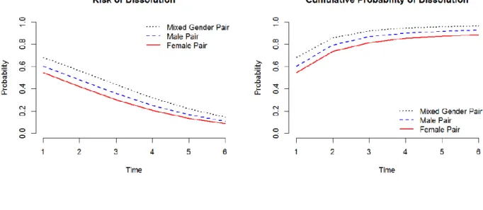
The sample observed hazard, survival, and lifetime distribution functions are plotted in
Figure 10, without modeling or accounting for the multiple membership dependence structure.
The hazard function indicates friendships are most likely to end at the first time period after the
friendship began, but if the friendship continues to exist it becomes less likely to end over time.
The sample observed functions also indicate that high school friendships in this sample are
highly fickle, in that 64% end after the first time period and only 8% are estimated to survive
from the start of high school until the end.
15 Although there are seven waves of collection, there are only six time periods for purposes of the data structure as
The FD Model is applied to longitudinal friendship nomination data using PQL through
SAS Glimmix, as the simulation study revealed a tendency for PQL to have less variable
parameter estimates albeit similar absolute bias for fixed and random effect recovery. Gender
and depression enter into the model as the main predictors of friendship dissolution.
Specifically, type of pair (males, females, mixed) is entered as two dummy-coded variables with
mixed as the reference group and depression is investigated both in terms of the average
depression of the pair as well as absolute difference in depression of the pair. Depression is
measured at each time period through a mood and feelings questionnaire (MFQ) as described in
Table 13 in Appendix A.1 (Costello & Angold, 1988).
As each individual has a time-varying depression score, and there are two individuals
within a pair, the effect of depression can be investigated multiple ways. Here, the average Figure 10: Sample estimated functions for high school friendship data.
Each pair has a mean depression score at each time period as well as an absolute difference in
depression at each time period, and there is variability both between pairs as well as within pairs.
In Figure 11, a sample of pairs’ scores are plotted where the numbers in the plots on the left
indicate the pair’s mean depression score (top) and the pair’s difference in depression score
(bottom) at each time period, and the dot indicates the pair’s average across time periods.
To investigate both within and between pair effects of depression, the pair’s mean depression
across time periods as well as each pair’s individual time period’s deviation from the pair’s mean
depression is entered into the model. Similarly, pair-mean centering is used to investigate the
influence of the absolute difference in the two individual’s depression scores. Thus, there are Figure 11: Depression.
formally four depression effects in the model: 1) average depression of the pair across time
periods, 2) pair’s time-specific deviation from their average depression, 3) average absolute
difference in the two individuals’ depression, and 4) pair’s time-specific deviation from their
average absolute difference in depression. The complexity of breaking down the effect of
depression in this way allows a more detailed view of the different ways depression of the two
individuals influence the pair’s likelihood of dissolution.
Results
As expected from the sample observed hazard functions, the model finds a high risk of
dissolution, yet a decreasing risk of dissolution over time. Thus, high school friendships in this
sample are very fickle, yet if they continue to last, they are less likely to end over time. For a
mixed gender pair with zero depression scores, the probability of dissolution by the first time
period after the friendship begins is 0.682 and although the risk of dissolving decreases over
time, the cumulative probability of remaining friends through six time periods is only 0.03. The
fixed effects are displayed below in Table 5 and the multiple membership effect is displayed
First examining the impact of depression, the average absolute difference in the two
individuals’ depression is found to have a positive relationship with the likelihood of dissolution,
F(1, 1280) = 4.63, p = 0.03. Thus pairs who have a larger absolute difference in depression
across time periods are more likely to end friendships across time than pairs who are more
similar in depression. However, no significant effect is found for the within-pair effect of the
difference in depression signifying there is not enough information to conclude a pair’s absolute
difference in depression changing over time relative to their average absolute difference is
related to their likelihood of dissolution when controlling for the other effects. Given so many
friendships end so quickly in this sample, it may be difficult for the model to pick out within-pair Table 5: FD Model Application – Fixed Effects.
Results from applying the FD Model to the high school friendship data.
Effect Estimate
Standard
Error DF t Value Pr > |t|
Intercept 1.269 0.190 612 6.670 <.0001
Time -0.507 0.062 1280 -8.180 <.0001
Male Pair (Mixed Gender Reference) -0.333 0.191 611 -1.740 0.0825
Female Pair (Mixed Gender Reference) -0.579 0.162 540 -3.580 0.0004
Pair Mean Depression -0.332 0.353 1280 -0.940 0.3481
Within Pair Mean Depression 0.482 0.551 1280 0.870 0.3818
Pair Mean – Absolute Difference Depression 0.629 0.292 1280 2.150 0.0316
Within Pair Difference Depression -1.516 0.900 1280 -1.690 0.0922
Significant effects at α=0.05 are in bold.
Table 6: FD Model Application – Covariance Parameter Estimates. Cov. Parameter Estimate Standard Error
effects.16 Similarly, there is no significant effect of average depression (within or between pairs)
on the likelihood of the friendship dissolving.
Holding depression constant, gender is found to have an influence on the likelihood of
dissolution, F(2, 255.6) = 6.43, p <0.01. Mixed-gender pairs have the highest likelihood of
dissolution, while female pairs are the least likely to dissolve friendships over time, as visualized
in Figure 12 below. The difference between the rate of dissolution for mixed-gender and female
pairs is significant, F(1, 540.1) = 12.85, p <0.01; this implies that females have 0.56 times as
high of odds of high school friendships ending at each time period than mixed-gender pairs,
holding the random effect at the population average. However, no significant difference between
male and female pairs is found, F(1, 127.8) = 1.96, p = 0.16, nor between male and
mixed-gender pairs, F(1, 610.8) = 3.02, p = 0.08.
16 Entering depression without separating into within and between pair effects results in a similar pattern as found
Figure 12: Friendship Dissolution by Gender.
Higher-level interactions between gender and time, gender and depression, and
depression and time were tested but not found to have significant effects. Accounting for the
effect of depression and gender in the model, the ICC as defined in the simulation study was only
0.02, revealing a very small correlation between the latent response variable for an individual
conditional on other individual’s friendship dissolution tendency. Given the findings of the
simulation study, however, it is likely that the random effect is actually underestimated here.
Conclusion
The FD Model introduced in this chapter allows an investigation of the processes leading
to friendship dissolution and gives insight into the typical length of friendships. The simulation
study revealed the model was able to recover the fixed effects reasonably well, with better
recovery with a larger number of nodes, a larger number of links per node, and smaller random
effect variance. The empirical application revealed insights into the timing of friendship
dissolution for a high school friendship network, leading to straightforward answers about how
long high school friendships typically last and the role of gender and depression in this process.
The FD Model includes a multiple membership random effect structure to account for
dependencies inherent in a social network in that individuals are members of multiple
relationships. Although the dependence structure found in the empirical example after
accounting for gender and depression effects was relatively weak, the FD Model is able to
account for this to allow investigation of the processes leading to friendship dissolution. In the
chapter that follows, another multilevel event history model is proposed, but this one with a
cross-classified membership structure to allow an investigation of the timing of reciprocity, as
Chapter 3: Reciprocal Timing (RT) Model
The motivation for the second proposed model is to answer questions about the processes
determining whether and when people reciprocate and will be denoted the “Reciprocal Timing”
(RT) Model. This model was motivated by an aim to understand the processes leading to
reciprocity and the timing of reciprocity on the social network site Twitter, which will be
investigated in the empirical example later in this chapter. The second model thus concerns the
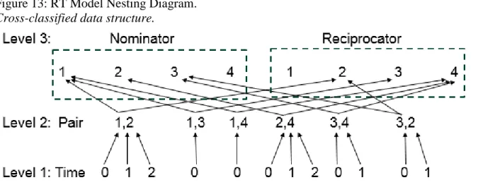
timing of reciprocal actions and in this case, we have pairs nested within a cross-classification of
nominators and reciprocators. The nominator is the individual who initiated the relationship
between the individuals of the pair and thus started the event duration process, and the
reciprocator has the opportunity to reciprocate the relationship. The duration between
nomination and reciprocity is studied, formally placing time at level 1, pairs at level 2, and
individuals (separated into nominator and reciprocators) at level 3, as visualized in Figure 13,
where time is conditional on the relationship formation. Some or all individuals will be