Recent Work
Title
Hydrodynamics of suspensions of passive and active rigid particles: A rigid multiblob approach
Permalink
https://escholarship.org/uc/item/1tt92276
Journal
Communications in Applied Mathematics and Computational Science, 11(2)
ISSN 1559-3940
Authors Usabiaga, FB Kallemov, B Delmotte, B et al.
Publication Date 2016
DOI
10.2140/camcos.2016.11.217
Peer reviewed
Particles:
A Rigid Multiblob Approach
Florencio Balboa Usabiaga,1 Bakytzhan Kallemov,1, 2 Blaise Delmotte,1
Amneet Pal Singh Bhalla,3 Boyce E. Griffith,3, 4 and Aleksandar Donev1,∗
1Courant Institute of Mathematical Sciences,
New York University, New York, NY 10012
2Energy Geosciences Division, Lawrence Berkeley National Laboratory, Berkeley, CA, 94720
3Department of Mathematics, University of North Carolina, Chapel Hill, NC 27599 4Department of Biomedical Engineering,
University of North Carolina, Chapel Hill, NC 27599
We develop a rigid multiblob method for numerically solving the mobility problem
for suspensions of passive and active rigid particles of complex shape in Stokes flow
in unconfined, partially confined, and fully confined geometries. As in a number of
existing methods, we discretize rigid bodies using a collection of minimally-resolved
spherical blobs constrained to move as a rigid body, to arrive at a potentially large
linear system of equations for the unknown Lagrange multipliers and rigid-body
mo-tions. Here we develop a block-diagonal preconditioner for this linear system and
show that a standard Krylov solver converges in a modest number of iterations that
is essentially independent of the number of particles. Key to the efficiency of the
method is a technique for fast computation of the product of the blob-blob
mobil-ity matrix and a vector. For unbounded suspensions, we rely on existing analytical
expressions for the Rotne-Prager-Yamakawa tensor combined with a fast multipole
method (FMM) to obtain linear scaling in the number of particles. For
suspen-sions sedimented against a single no-slip boundary, we use a direct summation on
a Graphical Processing Unit (GPU), which gives quadratic asymptotic scaling with
the number of particles. For fully confined domains, such as periodic suspensions
or suspensions confined in slit and square channels, we extend a recently-developed
rigid-body immersed boundary method [“An immersed boundary method for rigid
bodies”, B. Kallemov, A. Pal Singh Bhalla, B. E. Griffith, and A. Donev,
Commu-nications in Applied Mathematics and Computational Science, 11-1, 79-141, 2016]
to suspensions of freely-moving passive or active rigid particles at zero Reynolds
number. We demonstrate that the iterative solver for the coupled fluid and rigid
body equations converges in a bounded number of iterations regardless of the
sys-tem size. In our approach, each iteration only requires a few cycles of a geometric
multigrid solver for the Poisson equation, and an application of the block-diagonal
preconditioner, leading to linear scaling with the number of particles. We optimize
a number of parameters in the iterative solvers and apply our method to a variety of
benchmark problems to carefully assess the accuracy of the rigid multiblob approach
as a function of the resolution. We also model the dynamics of colloidal particles
studied in recent experiments, such as passive boomerangs in a slit channel, as well
as a pair of non-Brownian active nanorods sedimented against a wall.
I. INTRODUCTION
The study of the hydrodynamics of colloidal suspensions of passive particles is an old
yet still active subject in soft condensed matter physics and chemical engineering. In recent
years there has been a growing interest in suspensions of active colloids [1], which exhibit
rich collective behaviors quite distinct from those of passive suspensions. There is a growing
number of computational methods for modeling active suspensions [2–9], which are typically
built upon well-developed techniques for passive suspensions in steady Stokes flow, i.e., at
zero Reynolds number. Since active particles typically have metallic subcomponents, they
are often significantly denser than the solvent and sediment toward the bottom wall, making
it necessary to address confinement and implement non-periodic boundary conditions in
any method aimed at simulating experimentally-relevant configurations. Furthermore, since
collective motions seen in active suspensions involve large numbers of particles, and since
hydrodynamic interactions among particles decay slowly like the inverse of the distance, it
is crucial to develop methods that can capture long-ranged hydrodynamic effects, yet still
scale to tens or hundreds of thousands of particles.
For suspensions of passive particles the methods of Brownian [10, 11] and Stokesian
dynamics [12, 13] have dominated in chemical engineering, and related techniques have
been used in biochemical engineering [14–18]. These methods simulate the overdamped
(diffusive) dynamics of the particles by using Green’s functions for steady Stokes flow to
capture the effect of the fluid. While this sort of implicit solvent approach works very
well in many situations, it has several notable technical difficulties: achieving near linear
scaling for many-particle systems is technically challenging, handling non-trivial boundary
conditions (bounded systems) is complicated and has to be done on a case-by-case basis
[13, 19–28], generalizations to non-spherical (and in particular complex) particle shapes is
difficult, and including thermal fluctuations is non-trivial due to the need to obtain stochastic
increments with the desired covariance. In this work we develop relatively low-accuracy but
flexible and simple rigid multiblob methods that address these difficulties. Our approach
builds heavily on a number of existing techniques, combining elements from several distinct
but related methods. We extensively test the proposed methods and study their accuracy
and performance on a number of test problems.
The continuum formulation of the Stokes equations with suitable boundary conditions on
the surfaces of a collection of rigid particles is well-known and summarized in more detail in
Appendix A. Due to the linearity of the Stokes equations, there is an affine mapping from
the applied forces f and torques τ and any specified apparent slip velocity due to active
boundary layers ˘u, to the resulting particle motion given by the linear velocities u and the
angular velocities ω. Specifically,
u
ω
=N
f
τ
−N˘u˘, (1)
where N is the mobility matrix, and ˘N is an active mobility linear operator. The mobility
problem consists of computing the rigid-body motion given the applied forces and torques
and apparent slip. The inverse of this problem is the resistance problem, which computes
the forces and torques on the body given a specified motion of the body and active slip.
Solving the mobility problem is a key component of any numerical method for modeling the
deterministic or fluctuating (Brownian) dynamics of the particles.
in viscous fluid, specifically, we develop novel preconditioners for iterative solvers for the
unknown motions of the rigid bodies, given the applied external forces and torques as well
as active apparent slip on the surface of the particles. As we discuss in more detail in
the body of the paper, our formulation can readily solve the resistance problem; however,
our iterative solvers will prove to be more scalable for mobility computations (which are of
primary interest) than for resistance computations. Key to the success of our iterative solvers
is the idea that instead of eliminating variables usingexact Schur complements and solving
a reduced system iteratively, as done in the majority of existing methods [5, 29, 30], one
should instead iteratively solve an extended system that includes all of the variables. This
has the key advantage that the matrix-vector product becomes an efficient direct calculation,
and the Schur complement can be computed only approximately and used to construct an
effective preconditioner.
Like many other authors, we construct rigid bodies of essentially arbitrary shape as a
collection of rigidly-connected collection of “blobs” or “beads” forming a composite object
[29] that we will refer to as a rigid multiblob. The hydrodynamic interactions between blobs
are represented using a Rotne-Prager tensor generalized to the desired domain geometry
(boundary conditions) [31], specifically, we use the the Rotne-Prager-Yamakawa (RPY)
ten-sor [32] for an unbounded domain, and the Rotne-Prager-Blake (RPB) tenten-sor [13] for a
half-space domain. In Section II we describe how to obtain the hydrodynamic coupling
between a large collection of rigid multiblobs by solving a large linear system for Lagrange
multipliers enforcing the rigidity. A key contribution of our work is to develop an indefinite
saddle-point preconditioner for iterative solution of the resulting linear system. This
pre-conditioner is based on a block-diagonal approximation of the blob-blob mobility matrix, in
which all hydrodynamic interactions among distinct bodies (more precisely, among blobs on
distinct bodies) are neglected. The only system-specific component is the implementation
of a fast matrix-vector multiplication routine, which in turn requires a scalable method for
multiplying the RPY mobility matrix by a vector.
For simple geometries such as an unbounded domain or particles sedimented next to a
no-slip boundary, simple analytical formulas for the RPY tensor are well-known [13, 31], and can
be used to construct an efficient matrix-vector multiplication routine, for example, using fast
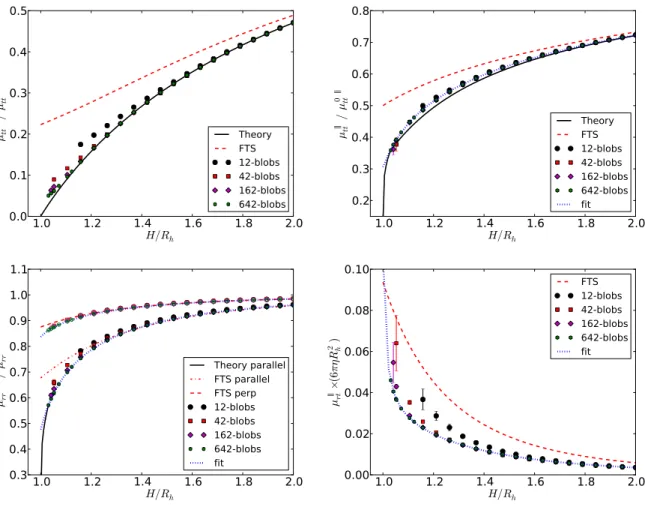
multipole methods (FMMs) [33, 34], or even direct summation on a GPU. We numerically
unbounded domain in Section IV, and study particles sedimented near a no-slip boundary in
Section V. We find that resolving spherical particles with twelve blobs placed on the vertices
of an icosahedron [35] is notably more accurate than the FTS (force-torque-stresslet plus
degenerate quadrupole) truncation typically employed in Stokesian dynamics simulations,
provided that the effective hydrodynamic radius of the rigid multiblob is adjusted to account
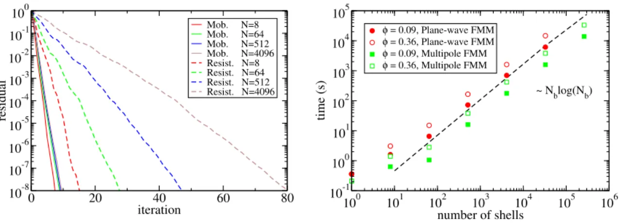
for the finite size of the blobs. We also find that a small number of iterations of a Krylov
method are required to solve the required linear system, and importantly, the number of
iterations is constant independent of the the number of rigid bodies, making it possible
to develop a linear or near-linear scaling algorithm. For resistance problems, however, we
observe a number of iterations growing at least as fast as the linear dimensions of the system.
This is consistent with similar studies of iterative solvers for Stokesian dynamics by Ichiki
[36].
For confined systems, however, even in the simplest case of a periodic system, the Green’s
function for Stokes flow and the associated RPY tensor is difficult to obtain in closed form,
and when it is possible to write an analytical result, the resulting formulas are typically
based on infinite series that are expensive to evaluate. For periodic systems this is commonly
addressed by using Ewald summation [37] based on the fast Fourier transform (FFT) [29]; the
present state-of-the-art for Stokes flow is the spectral Ewald method [25], which has recently
been used for Stokesian dynamics simulations of periodic suspensions [38]. A key deficiency
of most existing methods is that they rely critically on having triply periodic domains and
the use of the FFT. Generalizing these methods to non-periodic domains while keeping
their linear scaling requires a large development effort and typically a new implementation
for every different geometry [26, 28]. Furthermore, in a number of applications involving
active particles [39, 40], there is a surface slip (e.g., electrohydrodynamic or osmophoretic
flow) induced on the bottom boundary due to the gradients created by the particles, and
this slip drives or at least strongly affects the motion of the particles. Accounting for this
slip requires solving an additional equation such as a Poisson or Laplace equation for the
electric potential or concentration of chemical fuel with nontrivial boundary conditions on
the particle and wall surfaces. The solution of this additional equation provides the slip
boundary condition for the Stokes equations, which must be solved to find the resulting
fluid flow and active particle motion. Such nontrivial multi-physics coupling is quite hard
To address these difficulties, in Section III we develop a method for general cuboidal
confined domains which does not require analytical Green’s functions. This relies on an
im-mersed boundary (IB) method for obtaining an approximation to the RPY tensor in confined
geometries, as recently developed by some of us [41]. This technique has been combined with
the concept of multiblob representation of rigid bodies in a follow-up work [35], but in this
work stiff elastic springs were used to enforce the rigidity. By contrast, we ensure the rigidity
of the multiblobs via Lagrange multipliers which are solved concurrently with solving for
the fluid pressure and velocity. Our key novel contribution is an effective preconditioner
for the rigidly-constrained Stokes problem in periodic and non-periodic domains, obtained
by combining our recently-developed preconditioner for a rigid-body IB method [42] with a
block-diagonal preconditioner for the mobility subproblem.
In the IB method developed in Section III and studied numerically in Section VI,
analyt-ical Green’s functions are replaced by an “on the fly” computation carried out by a standard
finite-volume fluid solver. This Stokes solver can readily handle nontrivial boundary
condi-tions, for example, slip along the walls [39, 40] can easily be accounted for. Furthermore,
suspensions at small but nonzero Reynolds numbers can be handled with little extra work
[42, 43]. Additionally, we avoid uncontrolled approximations relying on truncations of
mul-tipole expansions to a fixed order [2, 12, 43, 44], and we can seamlessly handle arbitrary
body shapes and deformation kinematics. Lastly, and importantly, in the spirit of
fluctuat-ing hydrodynamics [41, 45, 46], it is straightforward to generate the stochastic increments
required to simulate the Brownian motion of small rigid particles suspended in a fluid by
including a fluctuating stress in the fluid equations, as we will discuss in more detail in
future work; here we focus on the deterministic mobility and resistance problems. At the
same time, our method also has some disadvantages compared to methods such as boundary
integral or boundary element methods. Notably, it requires filling the domain with a dense
uniform fluid grid, which is expensive at low densities. It is also a low-order method that
cannot compute solutions as accurately as spectral boundary integral formulations. We do
believe, nevertheless, that the method developed here offers a good compromise between
ac-curacy, efficiency, scalabilty, flexibility and extensibility, compared to other more specialized
formulations.
We apply our methods to a number of test problems for which analytical solutions are
the literature. In Section V B we study the mobility of a cylinder of finite aspect ratio that is
parallel to a no-slip boundary and compare to experimental measurements and asymptotic
theory based on a slender-body approximation. In Section V C we study the formation of
a stable rotating pair of active “extensor” or “pusher” nanorods next to a no-slip boundary,
and confirm the direction of rotation observed in recent experiments [47]. In Section VI D
we compute the effective diffusion coefficient of a boomerang-shaped colloid in a slit channel,
and compare to recent experimental measurements [48, 49]. In Section VI F we study the
mean and variance of the sedimentation velocity in a binary suspension of spheres of size
ratio two, and compare to recent Stokesian dynamics simulations [38, 50].
II. RIGID MULTIBLOB MODELS OF COLLOIDAL SUSPENSIONS
In this section we develop the rigid multiblob model of colloidal particles at zero Reynolds
number. The kind of models we use here are not new, but we present the method in detail
instead of relying on previous presentations, the most relevant of which are those of Swan
et al. [5, 29]. This is in part to present the formulation in our notation, and in part to
explain the differences with other closely-related methods. Our key novel contribution in
this section is the preconditioned iterative solver described in Section II B; the performance
and scaling of our mobility solver is studied numerically for unbounded domains in Section
IV D, and for particles confined near a single wall in Section V D.
The modeling of suspensions of rigid spheres at small Reynolds numbers is a
well-developed field with a long history. A powerful class of methods are related to Brownian
Dynamics with Hydrodynamic Interactions (BDHI) [10, 11, 51, 52] and Stokesian Dynamics
(SD) [12–14, 20, 38, 53] (note that these terms are used differently in different communities).
The difference between these two (as we define them here) is that BDHI uses what we call
a minimally-resolved model [41] in which each colloid (for colloidal suspensions) or polymer
bead (for polymeric suspensions) is only resolved at the monopole level, more precisely, at the
Rotne-Prager level [29]. By contrast, in SD the next level in a multipole expansion is taken
into account and torques and stresslets are also accounted for. It has been shown recently
that yet one more order needs to be kept in the multipole expansion to model suspensions of
active spheres [2, 8], and a suitable Galerkin truncation of the multipole hierarchy has been
near a no-slip boundary [9]. It is also possible to account for higher-order multipoles [8, 54–
57], leading to more complicated (and computationally expensive) but also more accurate
models. It has also been shown that multipole expansions converge very poorly for nearly
touching spheres due to the divergence of the lubrication forces, and in most methods for
dense colloidal suspensions of hard spheres pairwise lubrication corrections are added in a
somewhat ad hoc manner; we will refer to this approach as SD with lubrication.
Given the well-developed tools for modeling sphere suspensions, it is natural to leverage
them when modeling suspensions of particles of more complex shapes. Here we describe a
technique capable of, in principle, modeling passive rigid particles of arbitrary shape. The
method can also be used to model, without any extra effort, active particles with active
slip layers, i.e., particles which are phoretic (e.g., osmo-phoretic, electro-phoretic,
chemo-phoretic, etc.) due to an apparent slip at their surface. For the purposes of hydrodynamic
calculations, we discretize rigid bodies by constructing them out of multiple rigidly-connected
spherical “blobs” or beads of hydrodynamic radius a. These blobs can be thought of as
hy-drodynamically minimally-resolved spheres forming a rigid conglomerate that approximates
the hydrodynamics of the actual rigid object being studied. We prefer the word “blob”
over “sphere” or “point” or “monopole” because blobs are not spheres as they do not have
a well-defined surface like spheres do, they have a finite size associated with them (the
hydrodynamic blob radius a) unlike points, and they account for a degenerate quadrupole
associated to the Faxen corrections in addition to a force monopole. The word “bead” is
also appropriate, but we prefer to reserve that for polymer models (bead-spring or bead-link
models).
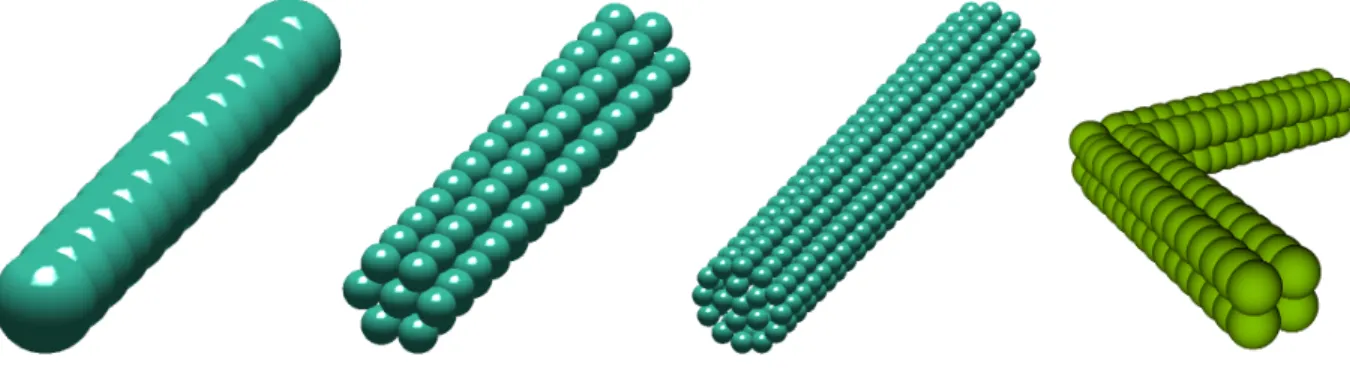
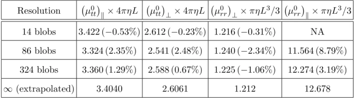
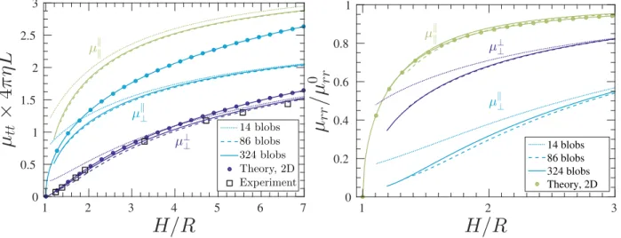
Examples of “multiblob” [35] models of two types of colloidal particles are illustrated in
Fig. 1. In the leftmost panel, we show a minimally-resolved model of a rigid rod, with
dimensions similar to active metallic “nanorods” used in recent experiments [47, 58]. In this
minimally-resolved model the blobs, shown as spheres with radius equal to a, are placed
in a row along the axes of the cylinder. Such minimally-resolved models are particularly
suited for cylinders of large but finite aspect ratio; for very thin rods such as actin filaments
boundary integral methods based on slender-body theory [59] will be more effective. In the
more resolved model illustrated in the second panel from the left, a hexagon of blobs is
placed around the circumference of the cylinder to better resolve it. A yet more resolved
Figure 1: Rigid multiblob models of colloidal particles manufactured in recent experimental work.
(Left three panels) A cylinder of aspect ratio of about six, similar to the active nanorods studied
experimentally in [47, 58], for three different resolutions; from left to right: minimally-resolved
model with 14 blobs, marginally-resolved model with 86 blobs, and well-resolved model with 324
blobs. (Rightmost panel) A 120-blob model of a boomerang with square cross-section, as studied
experimentally in [48].
panel from the left. In the rightmost panel of Fig. 1 we show a blob model of a colloidal
boomerang with a square cross-section, as manufactured using lithography and studied in
[48]. Similar “bead” or “raspberry” models appear in a number of studies of hydrodynamics
of particle suspensions [5, 6, 14–17, 35, 60–66].
In many studies, stiff elastic springs between the blobs are used to keep the structure rigid;
in some models the fluid or particle inertia is included also. Here, we keep the structures
strictly rigid and refer to the resulting structures as rigid multiblob models. Such rigid
multiblob models have been used in a number of prior studies [5, 14–17, 60, 64, 67], but we
refer to [5] for a detailed exposition. Our primary focus in this section will be to develop
algorithmic techniques that allow suspensions of tens or even hundreds of thousands of rigid
multiblob particles to be simulated efficiently. This is in many ways primarily an exercise
in numerical linear algebra, but one that isnecessary to make the rigid multiblob approach
useful for simulating moderately dense suspensions. A second goal, which will be realized in
the results sections of this paper, will be to carefully assess the accuracy of rigid multiblob
A. Hydrodynamics of rigid multiblobs
We now summarize the main equations used to solve the mobility and resistance
prob-lems for a collection of rigid multiblobs immersed in a viscous fluid. We first discuss the
hydrodynamic interaction between blobs, and then discuss the hydrodynamic interactions
between rigid bodies.
In the notation used below, we will use the Latin indices i, j, k, l for individual blobs,
and reserve Latin indices p, q, r, s for bodies. We will denote with Bp the set of blobs
comprising bodyp. We will consider a suspension of N rigid bodies with a chosen reference
tracking point on body p having position qp, and the orientation of body p relative to a
reference configuration represented by the quaternion θp [68]. The linear velocity of (the
chosen tracking point on) body p will be denoted with up, and its angular velocity will
be denoted with ωp. The total force applied on body p is fp, and the total torque is τp.
The composite configuration vector of position and orientation of body p will be denoted
with Qp = qp, θp , the composite vector of linear and angular velocity will be denoted
with Up ={up, ωp}, and the composite vector of forces and torques with Fp =
fp, τp .
The position of blob i ∈ Bp will be denoted with ri, and its velocity will be denoted with
˙
ri. When not subscripted, vectors will refer to the composite vector formed by all bodies
or all blobs on all bodies. For example, U will denote the linear and angular velocities of
all bodies, and r will denote the positions of all of the blobs. We will use a superscript
to denote portions of composite vectors for all blobs belonging to one body, for example,
r(p) ={r
i |i∈ Bp}will denote the vector of positions of all blobs belonging to body p.
The fact that the multiblob pis rigid is expressed by the “no-slip” kinematic condition,
˙
ri =up+ωp× ri−qp
, ∀i∈ Bp. (2)
This no-slip condition can be written for all bodies succinctly as
˙
r =KU, (3)
where K(Q) is a simple geometric matrix [29]. We will denote the apparent velocity of the
fluid at point ri with wi ≈ v(ri). For a passive blob, i.e., a blob that represents a passive
part of the rigid particle, the no-slip boundary condition requires that wi = ˙ri. However,
can be imposed, resulting in a nonzero slip u˘i = wi −r˙i. This kind of active propulsion
is termed “implicit swimming gait” by Swan and Brady [13]. An “explicit swimming gait”
[13] can be taken into account without any modifications to the formulation or algorithm by
simply replacing (2) with
wi = ˙ri =up+ωp×(ri−qp) + ˘ui. (4)
That is, the only difference between “slip” and “deformation” is whether the blobs move
relative to the rigid body frame dragging the fluid along, or stay fixed in the body frame
while the fluid passes by them. One can of course even combine the two and have the blobs
move relative to the rigid body while also pushing flow, for example, this can be used to
model an active filament where there is slip along the filament but the filament itself is
moving. In the end, the only thing that matters to the formulation is the velocity difference
˘
ui ≈v(ri)− up+ωp× ri−qp
. (5)
In Appendix C we explain how to model permeable (porous) bodies by making the apparent
slip proportional to the fluid-blob force λ.
The fundamental problem tackled in this paper is the solution of the mobility problem,
that is, the computation of the motion of the bodies given the applied forces and torques
on the bodies and the slip velocity. Because of the linearity of the Stokes equations and the
boundary conditions, there exists an affine linear mapping
U =NF −M˘ u˘,
where thebody mobility matrix N (Q) depends on the configuration and is the central object
of the computation. The active mobility matrix M˘ is a discretization of the active mobility
operator ˘N, and gives the active motion of force- and torque-free particles. Note that ˘M
is related to, but different from, the propulsion matrix introduced in [8]. The propulsion
matrix is essentially a finite-dimensional projection of the operator ˘N that only depends on
the choice of basis functions used to express the surface slip velocity ˘u, and does not depend
on the specific discretization of the body or quadrature rules, as does ˘M.
In the remainder of this section we develop a method for computing U given F and ˘u,
i.e., a method for computing the combined action of N and ˘M, for large collections of
we are given the motion of the bodies as a specified kinematics, and seek the resulting drag
forces and torques, which have the form
F =RU + ˘Ru˘,
where the body resistance matrix R = N−1 and ˘R = N−1M˘ is the active resistance matrix.
1. Blob mobility matrix
The blob-blob translational mobility matrix Mdescribes the hydrodynamic interactions
between the Nb blobs, accounting for the influence of the boundaries. Specifically, if the
blobs are free to move (i.e., not constrained rigidly) with the fluid under the action of set of
translational forces λi, the translational velocities of the blobs will be
w= ˙r+ ˘u =Mλ. (6)
The mobility matrix M is a block matrix of dimension (dNb) × (dNb), where d is the
dimensionality. Thed×dblock Mij computes the velocity of blob igiven the force on blob
j, neglecting the presence of the other blobs in a pairwise approximation.
To construct a suitable M, we can think of blobs as spheres of hydrodynamic radius
a. For two well-separated spheres i and j of radius a we have the far-field approximation
[13, 31, 52]
Mij ≈η−1
I +a
2
6∇
2
r0 I+
a2 6 ∇
2 r00
G(r0,r00)
r0=rj, r00=r
i, (7)
whereηis the fluid viscosity andGis the Green’s function for the steady Stokes problem with
unit viscosity, with the appropriate boundary conditions such as no-slip on the boundaries of
the domain. The differential operator I+ (a2/6)∇2 is called the Faxen operator [52]. Note
that the form of (7) guarantees that the mobility matrix is symmetric positive semidefinite
(SPD) by construction since G is an SPD kernel.
For a three dimensional unbounded domain with fluid at rest at infinity, the Green’s
function is isotropic and given by the Oseen tensor,
G(r0,r00)≡O(r =r0−r00) = 1 8πr
I +r⊗r
r2
. (8)
Using this expression in (7) yields the far-field component of the Rotne-Prager-Yamakawa
particles are close to each other to ensure an SPD mobility matrix [32], which can be derived
by using an integral form of the RPY tensor valid even for overlapping particles [31], to give
Mij =
1 6πηa
C1(rij)I +C2(rij)
rij⊗rij
r2 ij
, rij >2a
C3(rij)I +C4(rij)
rij⊗rij
r2
ij , rij ≤2a
(9)
where rij =ri−rj, and
C1(r) =
3a 4r +
a3
2r3, C2(r) =
3a 4r −
3a3
2r3,
C3(r) = 1−
9r
32a, C4(r) = 3r 32a.
The diagonal blocks of the mobility matrix, i.e., the self-mobility can be obtained by setting
rij = 0 to obtain Mii = (6πηa)
−1
I, which matches the Stokes solution for the drag on a
translating sphere; this is an important continuity property of the RPY tensor [69]. We will
use the RPY tensor (9) for simulations of rigid-particle suspensions in unbounded domains
in Section IV.
In principle, it is possible to generalize the RPY tensor to any flow geometry, i.e., to
any boundary conditions (and imposed external flow) [31], including periodic domains [37,
70], as well as confined domains [13, 20]. However, we are not aware of any tractable
analytical expressions for the complete RPY tensor (including near-field corrections) even
for the simplest confined geometry of particles near a single no-slip boundary. In the presence
of a single no-slip wall, an analytic approximation to Mij is given by Swan and Brady [13]
(and re-derived later in [71]) as a generalization of the Rotne-Prager (RP) tensor [32] to
account for the no-slip boundary using Blake’s image construction [72]. As shown in Ref.
[31], the corrections to the Rotne-Prager tensor (7) for particles that overlap each other but
not the wall are independent of the boundary conditions, and are thus given by the standard
RPY expressions (9) for unbounded domains. Therefore, in Section V we compute M by
adding to the RPY tensor (9) wall corrections corresponding to the translation-translation
part of the Rotne-Prager-Blake mobility given by Eqs. (B1) and (C2) in [13], ignoring the
higher order torque and stresslet terms in the spirit of the minimally-resolved blob model.
The expressions derived by Swan and Brady [13] assume that neither particle overlaps the
wall and the resulting expressions are not guaranteed to lead to an SPD M if one or more
For more complicated geometries, such as a slit or a square (duct) channel, analytical
computations of the Green’s function become quite complicated and tedious, and numerical
computations typically require pre-tabulations [20, 52, 73]. In Section VI we explain how a
grid-based finite volume Stokes solver can be used to obtain the action of the Green’s function
and thus compute the action of the mobility matrix for confined domains, for essentially
arbitrary combinations of periodic, free-slip, no-slip, or stress boundary conditions.
2. Body mobility matrix
After discretizing the rigid bodies as rigid multiblobs, we can write down a system of
equations that constrain the blobs to move rigidly in a straightforward manner. Letting λ
be a vector of forces (Lagrange multipliers) that acts on each blob to enforce the rigidity of
the body, we have the following linear system for λ, u, and ω for all bodies p,
X
j
Mijλj =up+ωp× ri−qp
+ ˘ui, ∀i∈ Bp, (10)
X
i∈Bp
λi =fp,
X
i∈Bp
(ri−qp)×λi =τp.
The first equation is the no-slip condition obtained by combining (6) and (2). The second
and third equations are the force and torque balance conditions for body p. Note that the
physical interpretation of λis that of a total force on the portion of the surface of the body
associated with a given blob. If one wants to think of (10) as a regularized discretization
of the first-kind integral equation (A5) and obtain a pointwise value of the traction force
density, one should divide λj by the surface area ∆Aj associated with blob j, which plays
the role of a quadrature weight [67]; we will discuss more sophisticated quadrature rules
[74, 75] in the Conclusions.
We can write the mobility problem (10) in compact matrix notation as a saddle-point
linear system of equations for the rigidity forces λ and unknown motionU,
M −K
−KT 0
λ
U
=
˘ u
−F
Forming the Schur complement by eliminating λ we get (see also Eq. (1) in [5] or Eq. (32)
in [29])
U =NF − N KTM−1
˘
u=NF −M˘ u˘,
where the body mobility matrix N is
N = KTM−1K−1
, (12)
and is evidently SPD since M is. Although written in this form using the inverse of M,
unlike in a number of prior works [14–16, 60, 64], we obtain U by solving (11) directly
using an iterative solver, as we explain in more detail in Section II B. We note that one can
compute a fluid velocity fieldv(r) from λ using a procedure we describe in Appendix B.
The resistance problem, on the other hand, consists of solving for λ in
Mλ=KU + ˘u, (13)
and then computing F =KTλ, giving
F = KTM−1K
U + KTM−1
˘
u =RU + ˘Ru˘.
At first glance, it appears that solving the resistance system (13) is easier than solving the
saddle-point problem (11); however, as we explain in more detail in Section IV D, the mobility
problem is significantly easier to solve using iterative methods than the resistance problem,
consistent with similar observations in the context of Stokesian Dynamics [36]. Observe
that the saddle-point formulation (11) applies more broadly to mixed mobility/resistance
problems, where some of the rigid body degrees of freedom are constrained but some are
free [76]. An example is a suspension of spheres being rotated by a magnetic field at a
specified angular velocity but free to move translationally, or a suspension of colloids fixed
in space by strong laser tweezers but otherwise free to rotate, or even a hinged body that can
only move in a partially-constrained manner. In cases such as these we simply redefine U
to contain the free kinematic degrees of freedom and modify the definition of the kinematic
matrix K. Much of what we say below continues to apply, but with the caveat that the
expected speed of convergence of iterative methods is expected to depend on the nature of
the imposed constraints, as we discuss in Section IV D.
Note that the formula (12) is somewhat formal, and in practice all inverses should be
surface of a body, the mobility matrix M is not invertible since making λ perpendicular
to the surface will not yield any flow because it will try to compress the (fictitious)
incom-pressible fluid inside the body. Note that this nontrivial null space of the mobility poses
no problem when using an iterative method to solve (11) because the right hand side is in
the proper range due to the imposition of the volume-preservation constraint (A6). It is
also possible that the matrix KTM−1K is not invertible. A typical example for this is the
minimally-resolved cylinder shown in the left-most panel of Fig. 1. Because all of the forces
λ are applied exactly on the semi-axes of the cylinder, they cannot exert a torque around
the symmetry axes of the rod. Again, there is no problem with iterative solvers for (11) if
the applied force is in the appropriate range (e.g., one should not apply a torque around the
semi-axes of a minimally-resolved cylinder).
B. Iterative Mobility Solver
For a small number of blobs, the equation (11) can be solved by direct inversion of M,
as done in most prior works. For large systems, which is the focus of our work, iterative
methods are required. A standard approach used in the literature is to eliminate one of the
variables λ orU. Eliminating λ leads to the equation
KTM−1K
U =F −KTM−1u˘, (14)
which requires the action of M−1, which must itself be obtained inside a nested iterative solver, increasing both the complexity and the cost of the method. Swan and Wang [29]
have recently used the Conjugate Gradient method to solve (14), preconditioning using the
block-diagonal matrixP = (6πηa) KTK .
An alternative is to write an equivalent system to (11), for an arbitrary constant c6= 0,
M −K
−KT (I+cM) c KTK
λ
U
=
˘ u
− F +cKTu˘
, (15)
from which we can easily eliminate U to obtain an equation for λ only, in the form
M I −K(KTK)−1KT
−c−1K(KTK)−1KT
λ= rhs, (16)
where we omit the full expression for the right hand side for brevity. The system (16) can
the simpler matrixKTK. Note that, although not presented in this way, this is the essence of
the approach that is followed and recommended by Swanet al. [5] (see Appendix [5] and note
that c is denoted by λ in that paper); they recommend computing the action of KTK−1 by an iterative method preconditioned by an incomplete Cholesky factorization. A similar
approach is followed in boundary integral formulations (which are usually formulated using
a double layer density), where a continuum operator related to K(KTK)−1KT is computed
and then discretized using a quadrature rule [27, 77].
In contrast to the approaches taken by Swanet al. [5, 29], we have found that numerically
the best approach to solving for the unknown rigid-body motions of the particles is to solve
the extended saddle-point problem (11) for both U and λ directly, using a preconditioned
iterative Krylov method. In fact, as we will demonstrate in the results section of this paper,
such an approach has computational complexity that is essentially linear in the number of
blobs because the number of iterations required to solve (11) is quite modest when an
appro-priate preconditioner, described below, is used. This approach does not require computing
(the action of) KTK−1
and leads to a very simple implementation.
1. Matrix-Vector Product
A Krylov solver for (11) requires two components:
1. An efficient algorithm for performing the matrix-vector product, which in our case
amounts to a fast method to multiply the dense but low-rank mobility matrix M by
a vector of blob forcesλ.
2. A suitable preconditioner, which is an approximate solver for (11).
How to efficiently compute Mλ depends very much on the boundary conditions and thus
the form of the Green’s function used to constructM. For unbounded domains, in this work
we use the Fast Multipole Method (FMM) developed specifically for the RPY tensor in [33];
alternative kernel-independent FMMs could also be used, and have also been generalized to
periodic domains [78]. The FMM method has an essentially linear computational cost of
O(NblogNb) for a single matrix-vector multiplication. In the simulations presented here we
solution process. Krylov methods, however, allow one to lower the accuracy of the
matrix-vector product as the residual is reduced [79]; this has recently been used to lower the cost
of FMM-based boundary integral methods [80]. We will explore such optimizations in future
work.
For rigid particles sedimented near a single no-slip wall, we have implemented a Graphics
Processing Unit (GPU) based direct summation matrix-vector product based on the
Rotne-Prager-Blake tensor derived by Swan and Brady [13]. This has, asymptotically, a quadratic
computational cost of O(N2
b); however, the computation is trivially parallel so the
multi-plication is remarkably fast even for one million blobs because of the very large number
of threads available on modern GPUs. Gimbutas et al. have recently developed an FMM
method for the Blake tensor by using a simple image construction (image Stokeslet plus a
harmonic scalar correction) and applying an infinite-space FMM method to the extended
system of singularities [34]. However, this construction has not yet been generalized to the
Rotne-Prager-Blake tensor, and, furthermore, the FMM will not be more efficient than the
direct product on GPUs in practice unless a large number of blobs is considered. For fully
confined domains, we will adopt an extended saddle-point formulation that will be described
in Section VI.
2. Preconditioner
In this work we demonstrate that a very efficient yet simple preconditioner for (11) is
obtained by neglecting hydrodynamic interactions between different bodies, that is, setting
the elements of M corresponding to pairs of blobs on distinct bodies to zero in the
pre-conditioner. This amounts to making a block-diagonal approximation of the mobility Mf
defined by only keeping the diagonal blocks corresponding to a single body interacting only
with the boundaries of the domain,
f
M(pq) =δpqM(pp). (17)
We will demonstrate here that the indefinite block-diagonal preconditioner,
P =
f
M −K
−KT 0
, (18)
Applying the preconditioner (18) amounts to solving the linear system
f
M −K
−KT 0
λ U = ˘ u −F
, (19)
which is quite easy to do since the approximate body mobility matrix (Schur complement),
f
N =KT
f
M−1K−1,
is itself a block-diagonal matrix where each block on the diagonal refers to a single body
neglecting all hydrodynamic interactions with other bodies,
f
Npq =δpq
K(p)T M(pp)
−1
K(p)
−1 .
ComputingNfpq requires a dense matrix inversion (e.g., Cholesky factorization) of the much smaller mobility matrix M(pp), whose size isdN(p)
b
×dNb(p), where Nb(p) is the number of blobs on body p. In the case of an infinite domain, the factorization of M(pp) can be precomputed once at the beginning of a dynamic simulation and reused during the simulation
due to the rotational and translational invariance of the RPY tensor; one only needs to
apply rotation matrices to the right-hand side and the result to convert between the original
reference configuration of the body and the current configuration. Furthermore, particles of
the same shape and size discretized with the same number of blobs as body p can share a
single factorization ofM(pp) and
f
Npp. In cases where M(pp) depends in a nontrivial way on
the position of the body, as for (partially) confined domains, one needs to factorize M(pp)
for all bodies pat every time step; this factorization can still be reused during the iterative
solve in each application of the preconditioner.
Because our preconditioner is indefinite, one cannot use the preconditioned Conjugate
Gradient (PCG) Krylov method to solve (11) without modification. One of the most robust
iterative methods, which we use in this work, is the Generalized Minimum Residual Method
(GMRES). The key advantage of GMRES is that it is guaranteed to reduce the residual
from iteration to iteration. Its main downside is that it requires storing a large number of
intermediate vectors (i.e., the history of the iterates). GMRES also can stall, although this
can be corrected to some extent by restarts. An alternative to GMRES is the (stabilized)
Bi-Conjugate Gradient (BiCG(Stab)) method, which works for non-symmetric matrices as
well. In our implementation we have relied on the PETSc library [81] for iterative solvers;
III. RIGID MULTIBLOBS IN CONFINED DOMAINS
The rigid multiblob method described in Section II requires a technique for multiplying
the blob-blob mobility matrix with a vector. Therefore, this approach, like all other Green’s
function based methods [8, 13, 20, 23–28, 52, 54–57], is very geometry-specific and does
not generalize easily to more complicated boundary conditions. To handle geometries for
which there is no simple analytical expression for the Green’s function, such as slit or square
channels, pre-tabulation of the Green’s function is necessary, and ensuring a positive
semi-definite mobility matrix is in general difficult. Another difficulty with Green’s function based
methods is that including a “background” flow is only simple when this flow can be computed
easily analytically, such as simple shear flows. But for more complicated geometries, such
as Poiseuille flow through a square channel, computing the base flow is itself not trivial or
requires evaluating expensive infinite-series solutions.
An alternative approach is to use a traditional Stokes solver to solve the fluid equations
numerically [11]. This requires filling the domain with a grid, which can increase the number
of degrees of freedom considerably over just discretizing the surface of the immersed bodies.
However, the number of fluid degrees of freedom can be held approximately constant as more
bodies are included, so that the methods typically scale very well with the number of particles
and are well-suited to dense particle suspensions. Previous work [41, 46, 82] has shown how
to use an immersed boundary (IB) method [83] to obtain the action of the Green’s function
in complex geometries. In this approach, spherical particles are minimally resolved using
only a single blob per particle. In subsequent work this approach was extended to multiblob
models [35], but the rigidity constraint was imposed only approximately using stiff springs,
leading to numerical stiffness. A class of related minimally-resolved methods based on the
Force Coupling Method (FCM) [30, 44, 45, 84] can include also torques and stresslets, as
well as particle activity [4], but a number of these methods have relied strongly on periodic
boundaries since they use the Fast Fourier Transform (FFT) to solve the (fluctuating) Stokes
equations.
In recent work [42], some of us have developed an IB method for rigid bodies. This
method applies to a broad range of Reynolds numbers. In the case of zero Reynolds number
it becomes equivalent to the rigid multiblob method presented in Section II, but with a
specified motion (kinematics) were considered; here we extend the method to handle
freely-moving rigid bodies in Stokes flow. We will present here the key ideas and focus on the new
components necessary to solve for the unknown motion of the particles; we refer the reader
interested in more technical details to Refs. [41, 42]. The key novel contribution of our
work is the preconditioner described in Section III C; the performance and scalability of our
preconditioned iterative solvers is studied numerically in Section VI E. To begin, we present
a semi-continuum formulation where the relation to Section II is most obvious, and then we
discuss the fully discrete formulation used in the actual implementation. In Appendix C we
demonstrate how to handle permeable bodies using a small modification of the formulation.
Numerical results obtained using the method described here are given in Section VI.
A. Semi-Continuum Formulation
We consider here a semi-discrete model in which the rigid body has already been
dis-cretized using blobs but a continuum description is used for the fluid, that is, we consider a
rigid multiblob model immersed in a continuum Stokesian fluid. In the IB literature blobs
are referred to as markers, and are often thought of as “points” or “discrete delta functions”.
We use the term “blob,” however, to connect to Section II and to emphasize that the blobs
have a finite physical and hydrodynamic extent.
In the IB method [83] (and also the force coupling method [84]), the shape of the blob and
its effective interaction with the fluid is captured through a smooth kernel function δa(r)
that integrates to unity and whose support is localized in a region of size comparable to the
blob radius a. In our rigid multiblob IB method, to obtain the fluid-blob interaction forces
λ(t) that constrain the unknown rigid motion of theNb blobs, we need to solve a constrained
blob constraint forces λ(t), and the unknown rigid-body motionsu(t) andω(t),
∇π =η∇2v+
Nb
X
i=1
λiδa(ri−r),
∇·v = 0,
Z
δa(ri −r0)v(r0, t)dr0 =up+ωp× ri−qp
+ ˘ui, ∀i∈ Bp, (20)
X
i∈Bp
λi =fp, ∀p,
X
i∈Bp
(ri−qp)×λi =τp, ∀p.
Note that here the velocity and pressure fields contain both the “background” and the
“per-turbational” contributions to the flow. In the first equation in (20), the kernel function is
used to transfer (spread) the force exerted on the blob to the fluid, and in the third equation
the same kernel is used to average the fluid velocity in the region covered by the blob and
con-strain it to follow the imposed rigid body motion plus additional slip or body deformation.
The handling of the spreading of constraint forces and averaging of the fluid velocity near
physical boundaries is discussed in Appendix D in [42]. We have implicitly assumed that
appropriate boundary conditions are specified for the fluid velocity and pressure. Notably,
we will apply the above formulation to cases where periodic or no-slip boundary conditions
are applied along the boundaries of a cubic prism (recall that periodic boundaries are not
actual physical boundaries). This includes, for example, a slit channel, a square channel,
or a cubical container. It is also relatively straightforward to handle stress-based boundary
conditions such as free-slip or pressure valves [85].
It is not difficult to show that (20) is equivalent to the system (10) with the mobility
matrix between two blobs i and j identified with [41, 42, 44, 45, 82, 84]
Mij(ri, rj) =η−1
Z
δa(ri−r0)G(r0,r00)δa(rj −r00)dr0dr00 (21)
where we recall thatGis the Green’s function for the Stokes problem with unit viscosity and
the specified boundary conditions. This expression can directly be compared to (7) after
realizing that for a smooth velocity field [44, 84],
Z
δa(ri−r)v(r)dr ≈
I+
Z x2
2 δa(x)dx
∇2
v(r)
r=ri =
I+ a
2
F
6 ∇
2
v(r)
where we assumed a spherical blob,δa(r)≡δa(r). We have defined here the “Faxen” radius
of the blob aF ≡ 3
R x2δ
a(x)dx
1/2
through the second moment of the kernel function.
In multipole expansion based methods, the self-mobility of a body is treated separately
by solving the single-body problem exactly (this is only possible for simple particle shapes).
However, in the type of approach followed here the self-mobility Mii is also given by the
same formula (21) with i = j and does not need to be treated separately. In fact, the
self-mobility of a particle in an unbounded three-dimensional domain defines the effective
hydrodynamic radius a of a blob,
Mii=
1
6πηaI =η −1
Z
δa(r0)O(r0 −r00)δa(r00) dr0dr00,
where the Oseen tensor O is given in (8). In general, aF 6= a, but for a suitable choice of
the kernel one can accomplish aF ≈a (for example, for a Gaussian a/aF =
p
3/π [84]) and
thus accurately obtain the Faxen correction for a rigid sphere [41].
For an isotropic or tensor product kernel δa and an unbounded domain, the pairwise
blob-blob mobility (21) will take the form
Mij =f(rij)I+g(rij) ˆrij⊗rˆij, (22)
whererij =ri−rj, and hat denotes a unit vector. The functions of distancef(r) andg(r)
depend on the specific kernel (and in the fully discrete setting on the spatial discretization
of the Stokes equations) and will be different from those appearing in the RPY tensor (9).
Nevertheless, as we will show numerically in Section VI A, the functions f and g for our IB
method are quite close in form to those appearing in the RPY tensor. We note that the
RPY tensor itself can be seen as a realization of (21) with the kernel being a surface delta
function over a sphere of radius a [31].
We have demonstrated above that solving (20) is a way to apply the blob-blob mobility
for a confined domain. In the method of regularized Stokeslets [23, 24, 67, 86] the mobility is
obtained analytically by averaging the analytical Green’s function with a kernel or envelope
function specifically chosen to make the resulting integrals analytical. Note however that
in that method the kernel δa appears only once inside the integral in (21) because only
the force spreading is regularized but not the interpolation of the velocity; this leads to
non-symmetric mobility matrix inconsistent with the Faxen formula (7). By contrast, our
approach is guaranteed to lead to a symmetric positive semidefinite (SPD) mobility matrix
B. Fully Discrete Formulation
To obtain a fully discrete formulation of the linear system (20) we need to spatially
discretize the Stokes equations on a grid. The spatial discretization of the fluid equation
used in this work uses a uniform Cartesian grid with grid spacingh, and is based on a
second-order accurate staggered-grid finite volume (equivalently, finite difference) discretization, in
which vector-valued quantities such as velocity, are represented on the faces of the Cartesian
grid cells, while scalar-valued quantities such as pressure are represented at the centers
of the grid cells [42, 43, 85, 87]. The viscous terms are discretized using a standard
7-point Laplacian (in three dimensions), accounting for boundary conditions using ghost cell
extrapolation [42, 85].
1. Spreading and interpolation
In the fully discrete formulation of the fluid-body coupling, we replace spatial integrals
in the semi-continuum formulation (20) by sums over fluid grid points. The regularized
delta function kernel is discretized using a tensor product of one-dimensional immersed
boundary kernelsφa(x) of compact support, following Peskin [83]. To maximize translational
and rotational invariance (i.e., improve grid-invariance) we use the smooth (three-times
differentiable) six-point kernel recently described by Bao et al. [88]. This kernel is more
expensive than the traditional four-point kernel [83] because it increases the support of the
kernel to 63 = 216 grid points in three dimensions; however, this cost is justified because the
new six-point kernel improves the translational invariance by orders of magnitude compared
to other standard IB kernel functions [88].
The interaction between the fluid and the rigid body is mediated through two crucial
op-erations. The discrete velocity-interpolation operatorJ averages velocities on the staggered
grid in the neighborhood of blob ivia
(Jv)αi =X
k
vkα φa(ri−rαk),
where the sum is taken over faces k of the grid, α indexes coordinate directions (x, y, z)
as a superscript, and rα
k is the position of the center of the grid face k in the direction α.
staggered grid via
(Sλ)αk = ∆V−1X
i
λαi φa(ri−rαk), (23)
where now the sum is over the blobs and ∆V = h3 is the volume of a grid cell. These
operators are adjoint with respect to a suitably-defined inner product, and the discrete
matrices satisfy J = ∆V ST, which ensures conservation of energy [83]. Extensions of the basic interpolation and spreading operators to account for the presence of physical boundary
conditions are described in Appendix D in [42].
We note that it is possible to change the effective hydrodynamic and Faxen radii of a
blob by changing the kernel δa. Such flexibility in the kernel can be accomplished without
compromising the required kernel properties postulated by Peskin [83] by using shifted or
split kernels [43],
φa,s(q−rk) =
1 2d d Y α=1 n φa h
qα−(rk)α−
s 2 i
+φa
h
qα−(rk)α+
s 2
io ,
where s denotes a shift that parametrizes the kernel. By varying s in a certain range, for
example, 0≤s ≤h, one can smoothly increase the support of the kernel and thus increase
the hydrodynamic radius of the blob by as much as a factor of two. We do not use split
kernels in this work but have found them to work as well as the unshifted kernels, while
allowing increased flexibility in varying the grid spacing relative to the hydrodynamic radius
of the particles.
2. Discrete constrained Stokes equations
Following spatial discretization, we obtain a finite-dimensional linear system of equations
for the discrete velocities and pressures and the blob and body degrees of freedom. For the
resistance problem, we obtain the following rigidly constrained discrete Stokes system [42],
A G −S
−D 0 0
−J 0 −Ω
v π λ =
g=0
h=0
w =−u˘ , (24)
where G is the discrete (vector) gradient operator, D = −GT is the discrete (vector)
finite-difference operators take into account the specified boundary conditions [85]. For
imperme-able bodies Ω = 0, which makes the linear system (24) a nested saddle-point problem in
both Lagrange multipliers π and λ. As explained in Appendix C, for permeable bodies Ω
is a diagonal matrix with Ωii =κp/(η∆Vi) for blob i∈ Bp, where κp is the permeability of
body p and ∆Vi is a volume associated with blob i. The right-hand side could include any
external fluid forcing terms, slip, inhomogeneous boundary conditions, etc. The system (24)
can be made symmetric by excluding the volume weighting ∆V−1 in the spreading operator (23); this makes λ have units of force density rather than total force.
This nested saddle-point structure continues if one considers impermeable rigid bodies
that are free to move, leading to thediscrete mobility problem 1
A G −S 0
−D 0 0 0
−J 0 0 K
0 0 KT 0
v π λ U = g
h=0
w =−u˘
z =F
. (25)
After eliminating the velocity and pressure from this system, we obtain the saddle-point
system (11) with the identification of the mobility with its discrete approximation
M=J L−1S = ∆V STL−1S, (26)
which is SPD. Here L−1 is a discrete Stokes solution operator,
L−1 =A−1−A−1G DA−1G−1
DA−1, (27)
where we have assumed for now thatA−1 is invertible; see [42] for the handling of periodic systems, for which the Laplacian is not invertible. Unlike for Green’s function based methods,
we never explicitly compute or formL−1orM; rather, we solve the Stokes velocity-pressure subsystems iteratively using the preconditioners described in [85, 89].
1 Note that in actual codes it is better to use an increment formulation of the linear system where the
C. Preconditioning Algorithm
In this section we describe how to solve the system (25) using an iterative solver, as we
have implemented in the Immersed Boundary Adaptive Mesh Refinement software
frame-work (IBAMR) [87]. Our codes are integrated into the public release of the IBAMR library.
Note that the matrix-vector product is a straightforward and inexpensive application of
finite-difference stencils on the fluid grid and summations over blobs. The key to an
ef-fective solver is the design of a good preconditioner, i.e., a good approximate solver for
(25). The basic idea is to combine a preconditioner for the Stokes problem [85, 89, 90] with
the indefinite preconditioner (18) with a block-diagonal approximation of the mobility Mf
constructed based on empirical fits of the blob-blob mobility, as we know explain in detail.
1. Approximate blob-blob mobility matrix
A preconditioner for solving the resistance problem (24) was developed by some of us in
[42]; readers interested in additional details should refer to this work. The preconditioner
is based on approximating the blob-blob mobility with the functional form (22), where the
functionsf(r) and g(r) are obtained by fitting numerical data for the blob-blob mobility in
an unbounded system (in practice, a large periodic system). This involves two important
approximations, the validity of which only affects theefficiency of the linear solver but does
not affect the accuracy of the method since the Krylov method will correct for the
approxi-mations. The first approximation comes from the fact that the true blob-blob mobility for
the immersed boundary method is not perfectly translationally and rotationally invariant,
so that the form (22) does not hold exactly. The second approximation is that the boundary
conditions are not correctly taken into account when constructing the approximation of the
mobilityMf. This approximation is crucial to the feasibility of our method and is much more
severe, but, as we will demonstrate numerically in Section VI, the Krylov solver converges
in a reasonable number of iterations, correctly incorporating the boundary conditions in the
solution.
The empirical fits of f(r) and g(r) are described in Appendix A of [42], and code to
evaluate the empirical fits is publicly available for a number of kernels constructed by
MobilityFunctions.c. As we show in Section VI A, these functions are quite similar to
those appearing in the RPY tensor (9), and, in fact, it is possible to use the RPY functions
fRP Y(r) and gRP Y(r) in the preconditioner, with a value of the effective hydrodynamic
ra-diusa that depends on the choice of the kernel. Nevertheless, somewhat better performance
is achieved by using the empirical fits for f(r) andg(r) developed in [42].
In [42], we considered general fluid-structure interaction problems over a range of
Reynolds numbers, and constructed Mf as a dense matrix of size (dNb)×(dNb), which was then factorized using dense linear algebra. This is infeasible for suspensions of many
rigid bodies. In this work, we use the block-diagonal approximation (17) to the blob-blob
mobility matrices, in which there is one block per rigid particle. Once Mf is constructed
and its diagonal blocks factorized, the corresponding approximate body mobility matrix Nf
is easy to form, as discussed in more detail in Section II B. Note that these matrices and
their factorizations need to be constructed only once at the beginning of the simulation, and
can be reused throughout the simulation.
2. Fluid solver
A key component of solving the constrained Stokes problems (24) or (25) is an iterative
solver for the unconstrained discrete Stokes sub-problem,
A G
−D 0
v π = g h ,
for which a number of techniques have been developed in the finite-element context [90].
To solve this system, we can use GMRES with a preconditioner P−1
S that assumes periodic
boundary conditions so that the various finite-difference operators commute [91].
Specif-ically, the preconditioner for the Stokes system that we use in this work is based on a
projection preconditioner developed by Griffith [85, 89],
P−1
S =
I h2G
f
Lp
−1
0 ηI
I 0
−D −I
η−1
f Lv −1 0 0 I
, (28)
where Lp = h2(DG) is the dimensionless pressure (scalar) Laplacian, and Lfv −1
≈ (Lv)
−1
and Lfp −1
≈(Lp)
−1
denote approximate solvers obtained by a single V-cycle of a geometric
In this paper we will primarily report the options we have found to be best without listing
all of the different combinations we have tried. For completeness, we note that we have tried
the better-known lower and upper triangular preconditioners [89, 90] for the Stokes problem.
While these simpler preconditioners are better when solving pure Stokes problems than the
projection preconditioner (28) since they avoid the pressure multigrid applicationLfp −1
, we
have found them to perform much worse in the context of suspensions of rigid bodies. A
possible explanation is that the projection preconditioner P−S1 is the only one that is exact for periodic systems if exact subsolvers for the velocity and pressure subproblems are used.
Observe that one application of P−S1 is relatively inexpensive and involves only (d + 1) scalar multigrid V-cycles. The number of iterations required for convergence depends
strongly on the boundary conditions; fast convergence is obtained within 10-20 iterations
for periodic systems, but as many as a hundred GMRES iterations may be required for
highly confined systems [89]. We emphasize that the performance of this preconditioner
is highly dependent on the details of the staggered geometric multigrid method, which is
not highly optimized in the hypre library, especially for domains of high aspect ratios such
as narrow slit channels. For periodic boundary conditions, one can use FFTs to solve the
Stokes problem, and this is likely to be more efficient than geometric multigrid especially
because FFTs have been highly optimized for common hardware architectures. However,
such an approach would require 3 scalar FFTs for each iteration of the iterative solver for
the constrained Stokes problem (24) or (25), and this will in general be substantially more
expensive than using only a few cycles of geometric multigrid as an approximate Stokes
solver.
The use of an approximate Stokes solver instead of an exact one is an important difference
between implementing the rigid multiblob method for periodic systems using the spectral
Ewald method [25, 38] and our approach. The product of the blob-blob mobility with a
vector can be computed more accurately and faster using the spectral Ewald method, in
particular because one can adjust the cutoff for splitting the computation between real and
Fourier space arbitrarily, unlike in our method where the grid spacing is tied to the
parti-cle radius. However, for rigid multiblobs, one must solve the system (11), which requires
potentially many matrix-vector products, i.e., many FFTs in the spectral Ewald approach.
By contrast, in our method we solve the extended problem (25), and only solve the Stokes
more iterations but each iteration can be substantially cheaper than performing three FFTs
each Krylov iteration. For non-periodic systems, there is no equivalent of the spectral Ewald
method, but see [11, 28] for some steps in this direction. Our method computes the
hydro-dynamic interactions in a confined geometry “on the fly” without ever actually computing
the action of the Green’s function exactly, rather, it is computed only approximately and
the outer Krylov solver corrects for any approximations made in the preconditioner.
3. Preconditioning Algorithm
We now have the necessary ingredients to compose a preconditioner for solving (25),
i.e., to construct an approximate solver for this linear system. Each application of our
preconditioner involves the following steps:
1. Approximately solve the fluid sub-problem,
A G
−D 0
˜ v
˜ π
=
g
h
,
using Ns(1) iterations of an iterative method with the preconditioner (28).
2. Interpolate ˜v to get the relative slip at each of the blobs, ˜w=Jv˜+w, and rotate the
corresponding component from the current frame to the reference frame of each body.
3. Approximately compute the unknown body kinematics U:
(a) Calculate ˜λ=Mf −1
˜
w and rotate the result back to the fixed frame of reference.
Here Mf is a block-diagonal approximation to the blob-blob mobility matrix in
the reference frame, as described in Section III C 1; the factorization of the blocks
of Mf is performed once at the beginning of the simulation.
(b) Calculate Fe =F+Kλ˜ and transform (rotate)Fe to the body frame of reference.
(c) Compute U =fNFe and transform it back to the fixed frame of reference, where
f
N =KMf
−1
KT−1.
4. Calculate the updated relative slip velocity at each of the blobs,