Singular light knots

Singular light knots

Andreani Petrou

THESIS

BACHELOR OF SCIENCE

in PHYSICS

Supervised by

Dr. Wolfgang Löffler & Dr. Jan Willem Dalhuisen (group of Prof. Dr. Dirk Bouwmeester)

Singular light knots

Andreani Petrou

Huygens-Kamerlingh Onnes Laboratory, Leiden University P.O. Box 9500, 2300 RA Leiden, The Netherlands

July 5, 2017

Abstract

Source-free Maxwell equations admit three-dimensional solutions with a knotted optical vortex structure. The theoretical evidence naturally gives rise to the question: Could such peculiar fields also exist in nature and in particular, could they be created in a laboratory? Our main objective is to provide an analytic investigation of their characteristic properties, which

will provide an insight in how their experimental synthesis could be achieved. A close examination reveals a saddle-shaped local polarization

pattern that is transverse everywhere to the vortex line and a broad spectral decomposition. Although the latter feature contradicts the

current experimental techniques and therefore complicates their realization; this thesis aims to bring the theory in closer contact with the

Contents

1 Introduction 1

2 Electromagnetic knots 3

2.1 Riemann-Silberstein vector 3

2.1.1 Superpotential Theory 4

2.1.2 Null fields 4

2.2 The electromagnetic Hopfion 5

2.2.1 The Bateman method 5

2.2.2 Whittaker-Synge construction 6

2.3 Phase Singularities 7

2.4 Algebraic knots and links 8

2.5 Knotted vortices in light fields 10

3 Characteristic properties of the knotted vortex fields 13

3.1 Polarization structure 13

3.1.1 The transverse plane 13

3.1.2 Polarization singularity 15

3.1.3 Saddle: Dynamical Systems approach 16

3.2 Color synthesis 19

3.2.1 Plane wave expansion 19

3.2.2 Spectral analysis 20

3.3 Invariants 23

3.3.1 Helicity 23

3.3.2 Constants of the motion 25

4 Towards experimental realization 28

4.1 Spectral modification 28

CONTENTS ii

5 Conclusion 32

Appendix A 34

Chapter

1

Introduction

After the suggestion by lord Kelvin in 1860 that atoms are knotted vortices of aether, a great mathematical interest in knots has stimulated the devel-opment of knot theory, a branch of modern topology. In the past decades, due to their unique property to endow stability, more and more applica-tions of knots appear in various physical systems such as fluid dynamics, field theory and the Penrose twistor theory [10]. The interest in this field has perceptibly increased after Rañada’s discovery [29] of the remarkable null solution to the source-free Maxwell equations with a non-trivial topol-ogy, known as the electromagnetic Hopf field. The name owes to its char-acteristic field line structure that resembles the Hopf fibration, in which any two electric or magnetic field lines are circles that are linked once. This field was investigated towards experimental realization by Irvine and Bouwmeester [16]. In a recent work by Kedia et al. [17], a broader fam-ily of knotted solutions is established in which the field lines encode torus knots of all types.

2

experimentally. During this process intriguing features emerge which can contribute in the field of classical and quantum optics.

Chapter

2

Electromagnetic knots

2.1

Riemann-Silberstein vector

In theoretical optics, and especially in the branch of singular optics, it is often practical to employ a complex combination of the electric and mag-netic field vectors, E and B, rather than treating them separately. This is achieved by introducing the Riemann-Silberstein (RS) vector

F(r,t) = E(r,t) +icB(r,t), (2.1)

where c is the speed of light, and its appearance in this expression serves for dimensional consistency, so that F is measured in units of the electric field (Newton per Coulomb in the SI system). The electric and magnetic field vectors are both real and they can be obtained by taking the real and imaginary parts of Equation 2.1. The advantage to be gleaned by this for-malism is that it does not only simplify calculations, but it also reveals an unequivocal correlation between the classical electromagnetic theory and quantum electrodynamics [9]. In addition, Eq. 2.1 can be naturally

generalized to the electromagnetic Faraday tensor Fµν and thus provides

a straightforward way to express Maxwell’s theory in the language of dif-ferential forms [11].

The source-free Maxwell’s equations in terms of the RS vector read

∇ ·F(r,t) =0, (2.2a)

i∂tF(r,t) =c∇ ×F(r,t). (2.2b)

2.1 Riemann-Silberstein vector 4

can be expressed in terms of vector potentialsC and AasE=∇ ×C and

B=∇ ×A, respectively. The potentials relate to each other, on account of the second equation, by

∇ ×C =−∂tA, ∇ ×A = 1

c2∂tC. (2.3)

Again we simplify the notation by combiningCand Ain a single complex

vector potential

V =C+icA, (2.4)

such that the RS vector is determined byF =∇ ×V.

2.1.1

Superpotential Theory

In an alternative formulation, due to Whittaker (1904) the RS vector is

ob-tained by the complexified Hertz potentialΠ[9], according to the formula

F(r,t) =

i

c∂t+∇×

(∇ ×Π(r,t)) (2.5)

Comparing this expression with the definition of the Riemann-Silberstein vector and using the relations in Eq. 2.3, we can identify a connection

between Π and a complex analogue of the electric potential, given by

e

C = ∇ ×Π, such that its curl and its time derivative will yield the real

and imaginary parts of F, respectively. The Hertz potential also bears the name superpotential, owing to the fact that the electromagnetic field is cal-culated by its second derivatives instead of the first. For this reason, there is a lot of freedom in choosing the vector superpotential, which can be re-duced by fixing its direction along a constant vectorm, such thatΠ =mΦ. Here Φ(r,t) is a complex scalar function, solution to the d’ Alambert (or wave) equation which satisfies(_c12∂2_t −∆)Φ(r,t) =0. It is called the

Whit-taker potential, or simply the scalar superpotential. For the sake of

sim-plicity in the following sections we use natural units by setting c = 1,

unless explicitly stated.

2.1.2

Null fields

Of particular interest are electromagnetic fields that can be classified as

2.2 The electromagnetic Hopfion 5

satisfied when both relativistic (Lorentz) invariantsS = E2−B2and P =

2E·Bvanish, or more compactly when the square of the RS vector satisfies

F·F =S+iP=0. (2.6)

Since the electromagnetic equations are unaltered in form under the action of the Lorentz group, the null property of the field persists in any inertial frame of reference. The interesting feature of null waves, is that their field lines∗ have preserved topology.

2.2

The electromagnetic Hopfion

Since their discovery, several studies have attempted to compose electro-magnetic knots using different formalisms. One of the most prominent is the Hopf-Rañada field, which we have briefly described in the introduc-tion and we denote byFH. It is a null field generated by the Hopf map (see

Ref. [21]) which is a continuous map from the 3-sphere to the 2-sphere and has topological (Hopf) index†equal to 1. The preimages of points inS2are circles inS3and are called the fibers of the map. At zero time, they can be

visualized in the compactified 3-space (which is simplyR3together with

a point representing infinity in all directions) via the stereographic projec-tion, which reveals that every pair of electric field lines are linked circles, lying on the surfaces of nested torii that fill up all space. The same ge-ometry is shared by the magnetic and Poynting vector field lines, oriented in perpendicular directions, forming the so called Hopf fibration. With time evolution, the field line and Poynting vector structure can deform while moving at the speed of light but the topology remains intact. In the current section we present two different mathematical prescriptions with which fields with these intriguing topological properties can be obtained.

2.2.1

The Bateman method

A method to constructnullelectromagnetic fields, was established by

Bate-man back in 1915 [4] and it is widely known as the BateBate-man construction.

∗_{With field lines we refer to the integral curves of the electric (or magnetic) vector}

field at a chosen instance in time (restricted to a space-like slice of the Minkowski space), which are solutions of the differential equation ˙r = E(r) (sim. for B), where the dot denotes the derivative with respect to a parameter.

†_{A formal definition of the index in terms of the Brouwer degree of a map is provided}

2.2 The electromagnetic Hopfion 6

According to this method and as proven in Ref. [15], any field F

bear-ing the null property (i.e. satisfies Eq. 2.6) can be expressed in terms of two smooth complex-valued functions of the Minkowski (space-time) variablesα,β: M →Cwhich satisfy the condition

∇α× ∇β=i(∂tα∇β−∂tβ∇α).

Such α,β are called the Bateman variables and the Riemann-Silberstein

vector can be obtained by the cross product of their gradients according to

F =∇α× ∇β. (2.7)

In this formulation, the Hopfion FH can be generated by the choice ofα

and βthat was suggested by Kedia et. al. [17], which can be expressed as

functions of the spatio-temporal coordinates in the explicit form

α(r,t)=r

2_−a2_−t2_+2iaz

r2_−(t−ia)2 , (2.8a)

β(r,t)= 2a(x−iy)

r2_−(t−ia)2, (2.8b)

where r2 = x2+y2+z2 and a is a real constant. Observing that |α|2+

|β|2 = 1, this choice of (α,β) is special since at zero time(t = 0) it

coin-cides with the inverse stereographic projection from a space-like slice of Minkowski space (isomorphic toR3) to the 3-sphereS3. It is important to note that to ensure this correspondence, a rearrangement of coordinates in the standard stereographic formula (see e.g. Ref. [21]) is required. By sub-stituting these expressions in Equation 2.7, the RS vector for the Hopfion acquires the form

FH(r,t) = 4

a2

(r2_−(t−ia)2₎3 



−(x−iy)2+ (z−(t−ia))2

i((x−iy)2+ (z−(t−ia))2)

−2(x−iy)(z−(t−ia))



. (2.9)

2.2.2

Whittaker-Synge construction

In an extension of the superpotential theory by Whittaker, Synge [32] has

proposed to buildnullMaxwell’s solutions by the second derivatives of a

scalar wave function (analogous toΦintroduced above). This reproduces

2.3 Phase Singularities 7

χH(r,t) =

4a2

r2_−(t−ia)2 (2.10)

according to Eq. A.1 given in Appendix A. It is (up to a scaling factor)

a generalization of the elementary solution to the wave equation (r2−

t2)−1, in which the shift of the time variable by a constant complex term is introduced to eliminate the singularity from the light cone, i.e. when

r2−t2 = 0. This also elucidates the appearance of a in the definition of the Bateman variables, which ensures that the Hopf field (Eq. 2.9) is non-singular at all points in space-time. By settinga=1, the above expressions reduce to the familiar form used in previous literature, but for reasons to

be later clarified, we retain a more general form in which acan take both

positive and negative values.

Before proceeding with the development of an analytical setting that allows fields withknotted optical vorticesin section 2.5, let’s pause to clar-ify what we mean by these terms, which we have already encountered in the introduction. In the following section we provide a brief description of an optical singularity, while Section 2.4 is dedicated to an elementary introduction to knots and links and their polynomial representation.

2.3

Phase Singularities

As defined in a Singular Optics review by Dennis et al. [14], a phase

singularityis a scalar optical phenomenon that occurs at points where the intensity of a complex scalar field vanishes and the phase is undefined;

hence it is singular. To make this more transparent, a scalar field ψ can

be written in the polar form ψ = ρeiδ in terms of a real phase δ and

am-plitude ρ (the intensity then reads I = ρ2). It is obvious that the phase

fails to be defined when ψ = 0, in a similar manner as the polar angle

is undefined at the origin. The name optical vortex owes to the fact that such singular points are vortices in the optical current−or energy−flow, which is carried by the Poynting vectorS. They can be viewed as the posi-tion in space around which the wavefronts (surfaces of equal phase) form a helical structure, with phase labels ranging from 0 to 2π. For this

rea-son, optical vortices are also known as wavefront dislocations and they are intriguing features in electromagnetism since the topology of the sur-rounding field is determined by the topology of the singularity.

2.4 Algebraic knots and links 8

expressing the electric and magnetic field vectors in their complex repre-sentation (in which the physical field corresponds to the real part only) such that each of their components can independently posses a phase sin-gularity. It is important to stress that in this scheme the total intensity of the field does not necessarily vanish at the vortex points and thus makes them hard to recognize experimentally. Another drawback of this descrip-tion, is that it treats Eand B separately and thus the singularities are not relativistic invariant and it also relies on their complex character. The lat-ter is incompatible with the Riemann-Silberstein formalism as introduced in Sec. 2.1, where the fields are represented by real vectors. An alterna-tive description was thereby proposed by Bialynicki-Birula [8] in which the optical vortex is associated with the vanishing set of the square of the RS vector. The scalar field is thus written asψ= F·Fand the

correspond-ing phase, given by the argument arg(F·F), is singular at the zero’s of

F(r,t)·F(r,t) = S+iP. These are 1-dimensional lines in 3-space

occur-ring at the intersection of the surfaces S = 0 and P = 0 [5, 7]. In

con-sequence, the electromagnetic field is null along the dislocation lines (c.f Eq.2.6).

In the special case of vortices in paraxial fields (such as Laguerre-Gaussian beams; they consist of plane waves with propagation directions spanning small angles with respect to the z-axis), the optical current contains an

azimuthal component of the form ei`φ_{. This term induces a net flow of}

energy and momentum circulating around the vortex line, endowing the

field with orbital angular momentum. The real quantity`is known as the

topological charge and takes only integer values that give a characteris-tic measure of the “strength” of the singularity. Moreover, depending on its sign, the singularity can be classified as right-handed (` > 0) or left-handed (` <0).

2.4

Algebraic knots and links

In the usual sense a knot refers to an intertwined linear material (a piece of string, say) that it is tied into itself, finding various applications in ev-ery day life, under circumstances where boundedness is required (ranging from tying shoelaces to sailor practices). Their mathematical definition does not deviate much from this description, with the only difference

be-ing that they are made of a sbe-ingle closed loop which need not be tightly

confined in space, but rather can extend to reveal its topological proper-ties. Two or more closed loops tangled together form what we call a link.

2.4 Algebraic knots and links 9

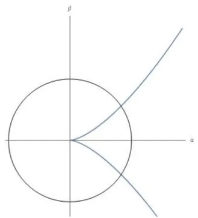
C in 2 complex variables that has a cusp singularity at the origin

(imply-ing that its partial derivatives vanish there; see Fig. 2.1). In addition, we require that it has a vanishing constant term such thath(0, 0) = 0, and for a choice of non-zero coefficientsλrs eRand(u,v)eC2it can be written in

the general form

h(u,v) =

∑

r

∑

λrsurvs. (2.11)

Its zero set, is referred to as a complex plane curve and consists of all the pairs (u,v)inC2that satisfy h(u,v) = 0. The intersection of this zero set with the 3-sphere (S3 ⊂ C2_{) that is centered at the origin of R}4

e

=C2, is denoted by V = {(u,v)e S3 | h(u,v) = 0}and encodes an algebraic knot

or link lying onS3. It is hard to visualize this since it lies in a 4-dimensional space but it can be schematically represented in the plane, by viewing each axes as the complex plane C. This is depicted in Figure 2.1. Note that the components (or loops) of such a link uniquely correspond to irreducible

factors of the polynomial h, while a knot (1-component link) is obtained

when hitself is irreducible [12].

Figure 2.1: Schematic representation ofC2_{in a 2-dimensional plane showing the} 3-sphere (circle) and the zero set of the polynomial (cusp). The 2 points of inter-section in this configuration, correspond to a torus knot lying on the 3 sphere in a 4-dimensional space.

In the current work, we focus on the particular case oftorusknots (and links) characterized by a pair of integers (p,q) and a polynomial of the formh(u,v) = λp0up+λ0qvq. With this choice,Vrepresents a knot whenp

andqare coprime and otherwise it is a link (for example the Hopf link

cor-responds to p=q =2). This is made more intuitive for our 3-dimensional

2.5 Knotted vortices in light fields 10

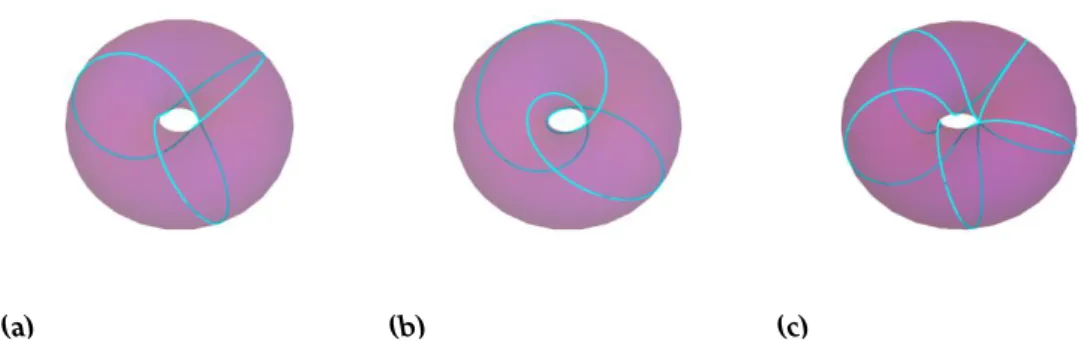
number of windings in the toroidal and poloidal direction, respectively, as illustrated in Figure 2.2. From the trefoil example considered in parts (a) and (b), it is obvious that, although knots obtained by interchanging their directed number of windings are geometrically dissimilar, they share the same topology. Additionally, it can be observed that the number of times the curve wraps around the torus passing through its hole, yields a

q-fold azimuthal symmetry. A scrupulous description of such knots and

their topological properties is given in Chapter 5 of Ref. [1], although there (and in their traditional definition) the roles of pandqare interchanged.

(a) (b) (c)

Figure 2.2: Parametric plots of the (a),(b) trefoil and (c) cinquefoil knots embed-ded on the standard torus with corresponding(p,q)pairs equal to: (a)(2, 3); the curve wraps twice along the long way around the torus (toriodal direction) and 3 times through the hole of the torus (poloidal direction), (b)(3, 2); now the number of windings in poloidal and toroidal directions are interchanged, but the resulting knot has the same topology and (c)(2, 5);2 toroidal and 5 poloidal windings form the cinquefoil knot on the torus. Its(5, 2)counterpart has a similar symmetry as in case (b).

In an extension of this classification to cable, or iterated torus knots, the zero set of the polynomial can be obtained by an algorithm, called

the Newton expansion, which expressesvin terms of fractional powers of

u in successive approximations, such that a finite number of pairs (p,q)

determine the total topology of the knot. Further details are beyond the scope of this thesis but can be found in Ref. [12].

2.5

Knotted vortices in light fields

We have already studied a special case of an electromagnetic knot, the

2.5 Knotted vortices in light fields 11

that do not vanish simultaneously anywhere in space-time. However, in the present work our main objective is to consider 3-dimensional electro-magnetic vector fields that encompass a knotted (or linked) zero-intensity line.

Although in Section 2.3 we have introduced the notion of an optical vortex as a scalar phenomenon, it has been demonstrated [7] that this

def-inition can be generalized to the case of a null vector field in vacuum.

In particular, a phase singularity can be implemented in a 3-dimensional background field that satisfies the null condition, via its multiplication with a complex scalar function. In this manner, the points of zero intensity

−at which all the components of the resulting field vanish, are governed

by the zero set of this function, forming an isolated 1-dimensional curve along which the phase is undefined. We restrict our attention in generat-ing vortex lines with the topology of algebraic knots and links, built upon the Hopfion solution, which is indeed null (as established in Ref. [6]) and constitutes the basis of our construction. This is achieved by exploiting the

property of the Bateman construction which allows the replacement of α

and βin the formula 2.7 with two arbitrary holomorphic functions of the

Bateman variables∗ f, g: C2 →Csuch that

F(r,t) = ∇f(α,β)× ∇g(α,β) = (∂αf∂βg−∂βf∂αg)∇α× ∇β is still a null field. Adapting the method proposed in [12], we comprise

the polynomialhof the previous section in this formalism, by making the

specific choice f(α,β) = R h(α,β)dαand g(α,β) = βsuch that

F(r,t) = h(α,β)∇α× ∇β. (2.12)

This expression clearly vanishes at the points(α,β)which satisfyh(α,β) =

0, and since such points lie on the 3-sphere, this gives precisely the knotted curve that we desire to embed as an optical vortex into the Hopfion. In the specific case of (p,q) torus knots vortices, the Riemann-Silbertein vector, obtained by writinghin the form 2.11, reads

Fpq(r,t) =

∑

λrsFrs(r,t), (2.13)

where

Frs(r,t) =αrβsFH(r,t). (2.14)

∗_{To give the Hopf as background field we refer to the explicit form ofα,βas given in}

2.5 Knotted vortices in light fields 12

Note that Equation 2.13 reduces to FH when the only non-vanishing

co-efficient corresponds to r = s = 0. Moreover, for the choice λrs = pq

when r = p−1 and s = q−1, the fields Frs bear a close resemblance

to the (p,q)-knotted waves proposed in [17] that were mentioned in the introduction (the torus knots appear in their field line rather than vortex structure). This notation will be convenient in our attempt to obtain the

Chapter

3

Characteristic properties of the

knotted vortex fields

3.1

Polarization structure

In order to experimentally build the topologically non-trivial fields pre-sented in the preceding chapter, the natural next step is to examine several of their characteristic features. Of particular importance is the local po-larization of these fields, which is to say, their field line behavior in the vicinity of the vortex line. We devote this section to the investigation of only the electric field, but due to their close connection imposed by the nullness condition, a similar description applies to the magnetic field.

3.1.1

The transverse plane

We begin our treatment with the choice of polynomial h(α,β) = 2p/2αp+

2q/2

βq. Restricted tot = 0, we obtain a parametrizationγ for the knotted

vortex line in terms of a parameter ϑ that ranges from 0 to 2π. This is

achieved by substituting α = √1₂eiqϑ inh(α,β) = 0 to get a point ˜γ(ϑ) = 1

√ 2(e

iqϑ_,ei(pϑ+π/q)_{)on the 3-sphere(}S3_⊂C2_{), which can then be identified}

with R3 via the stereographic projection Π : S3 → R3. This is such that when projecting from the north pole, every 4-tuple (u1,u2,u3,u4) e S3 is

mapped to _1−u1

1(u3,−u4,u2). The parametrizationγ = Π◦γ˜ : [0, 2π] → R3_{then takes the form}

γ(ϑ)=√ 1

2−cos(qϑ)

cos

pϑ+π

q

,−sin

pϑ+π

q

, sin(qϑ)

3.1 Polarization structure 14

which is a curve in R3 corresponding to the (p,q) knotted zero-intensity line as embedded in the fields viah(α,β), according to Equation 2.12. This

is assured by the explicit form of the stereographic projection, in which the coordinates are rearranged such that to agree with the form of(α,β)at t=0 as defined by Equations 2.8.

We now restrict our attention to the field-line behavior in the trans-verse plane, which is perpendicular to the vortexγfor everyϑ e[0, 2π]. To

accomplish this we introduce the curvilinear coordinate system, denoted by primed coordinates(x0,y0,z0), which is obtained by computing the

tan-gentt, normalnand binormal bunit vectors of the parametrization. The

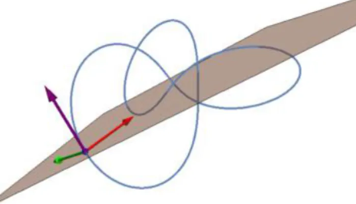
last two vectors span the transverse plane which is orthogonal to the tan-gent(t =n×b)at each point along the curved vortex. Together they form an oriented orthonormal basisB ={n,b,t}as depicted in Fig. 3.1.

Figure 3.1: Parametric plot of the trefoil (2,3) knot. At the point corresponding to ϑ = 2π₃ , the purple arrow represents the tangent vector t and the red and

green arrows represent the normal n and binormalb, respectively, which span the transverse plane (orthogonal to the vortex), forming an oriented orthonormal basisB={n,b,t}.

Subsequently, we perform a coordinate transformation consisting of a translation of the origin to a pointγ(ϑ)lying on the vortex line, followed

by a rotation, which aligns (in an oriented way) the z-axis of the primed

3.1 Polarization structure 15

C(r−γ(ϑ)), whereCis the change of basis matrix from the standard basis

inR3to the basisB∗. After writing the electric field in terms of the primed coordinates, we express it with respect to the new basis asE0(r0) = CE(r0). By construction, this vanishes at the new origin (atr0 =0) which is placed on the singularity. For convenience we omit the primes in the discussion hereafter, while working explicitly with the primed field and coordinate system.

3.1.2

Polarization singularity

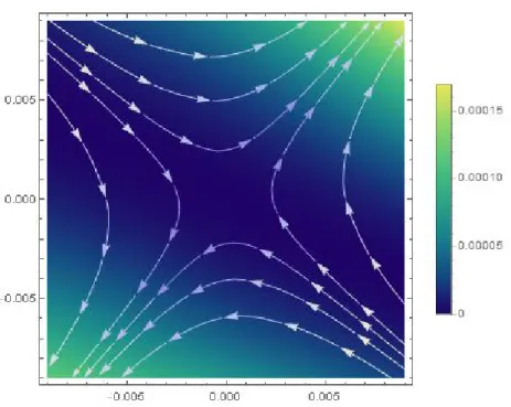
Our analysis proceeds by visualizing the transverse electric field-line struc-ture in the vicinity of the optical vortex. Using the computer algebra sys-tem Wolfram Mathematica, we plot the field lines of the vector fields in the xy-plane (of the primed system) positioned at a reference point lying on the vortex line. The result is a saddleshaped local polarization pattern, as demonstrated in Figure 3.2. This figure also includes a density plot of the z-component contribution of the field (perpendicular to the plane), reveal-ing that it is locally very small −as to be anticipated since it points along the singular direction. In fact, it is negligible since similar plots of the x and y component contributions assure that it is at least 2 orders of mag-nitude smaller, and therefore we can assume a polarization that is purely transverse to the vortex.

From the configuration appearing in the field line plot, at the center of the saddle (dislocation point) the polarization fails to be defined, and therefore it is singular there. This is a natural consequence of the way the definition of a phase singularity was extended to encompass the vectorial nature of null fields (see Sec. 2.5): at a zero intensity point the polarization can not be specified. It should be remarked, that the notion of polarization singularity arising in this context, does not coincide with the traditional definition as introduced by Nye and Hanjal [26]. In their seminal paper, they target single-frequency waves and assert that their vector singular-ities are lines of purely circular or linear polarization, along which the electric (or magnetic) vibration ellipse is undefined. Although the latter is not associated with vanishing intensity, the parallelism between the two concepts, is an interesting alley that deserves further investigation.

In order to assure that this behavior has a global character (i.e. that it occurs at all vortex points), we animate the above plots by varying the

parameter ϑ. The outcome has demonstrated that the saddle of Figure

3.1 Polarization structure 16

Figure 3.2: For an optical vortex in the shape of the trefoil-(2,3) knot we plot the field lines of the electric field in the transverse plane, about the vortex point corresponding toϑ= π₂, which is placed at the origin of our coordinate system. In

the background a density plot shows that the z-component of the field (pointing out of the page) is effectively zero when comparing with the x,y contributions (not shown here).

3.2 appears as the transverse polarization portrait in the vicinity of every reference point, but exhibits a rotation about the origin. This is closely re-lated to the in-plane rotation of the normal and binormal vectors as the tangent rides along the optical vortex. In the next subsection, after devis-ing a mathematical model corresponddevis-ing to this system, we shall present a more detailed description of this rotatory behavior. Worth mentioning is that the "global" transversal character we have observed is a familiar fea-ture in the well known field of paraxial optics, and thus could facilitate the endeavor of creating them in the lab.

3.1.3

Saddle: Dynamical Systems approach

In a mathematical viewpoint, we use tools from dynamical system the-ory (see Ref. [22]) in order to classify the local behavior of the electric field lines in the neighborhood of the equilibrium. This is defined as the pointp

3.1 Polarization structure 17

indeed occurs at the origin of our new coordinate system (remember that we omit the primes). The electric field lines are the integral curves (see the first footnote on page 5) of a smooth vector field, and thus can be consid-ered as the flows of the dynamical system ˙r = E(r), where the derivative is with respect to the vortex parameter ϑ. Often this behavior is fully

de-termined by the linearization∗of the system ˙r = Mr, whereM=DE(p)is the Jacobian matrix of Eat the point p, with components Mij = DjEi(p).

Note that in this case the z axis is tangent to the optical vortex, so that the derivative of all 3 components of the field, which are independent, vanish along that direction, i.e. ∂zEx(p) = ∂zEy(p) = ∂zEz(p) = 0.

Addition-ally, the divergence-free condition implies that the trace of the matrix Mis equal to zero, giving the relation ∂yEy(p) = −∂xEx(p). Taking these into

account, we can write the linearization matrix as

M =





∂xEx(p) ∂yEx(p) 0

∂xEy(p) −∂xEx(p) 0

∂xEz(p) ∂yEz(p) 0 

.

Clearly this matrix has a zero eigenvalue, which classifies the equilib-rium point pas non-hyperbolic†. Therefore the linearization (or Hartman-Grobman) theorem, which assures that the flows of the original and the linearized system are topologically conjugate (homeomorphic) in a neigh-borhood of a hyperbolic equilibrium, and thus establishes that the linear analysis gives a sufficient description of the non-linear dynamical behav-ior, is not applicable in this case.

To overcome this issue, we restrict our treatment to the 2 dimensional equivalent of the aforementioned system, in which we consider the projec-tion of the E-field onto the transverse plane, such thatE → E⊥ = Ex,Ey

e R2. This is reasonable as long as we stay within a small enough

neigh-borhood around the equilibrium point p, and since the z-component

con-tribution of the field Ezis negligible compared to the 2 transverse

compo-nents, as demonstrated via the Mathematica simulations of the previous section. In this case, the linearization matrix becomes

M⊥ =

∂xEx(p) ∂yEx(p)

∂xEy(p) −∂xEx(p)

.

∗_{The linearization method is equivalent to a Taylor expansion −up to linear terms,}

as suggested by its name−which gives an approximate description of the behavior of a function in the vicinity of a point.

3.1 Polarization structure 18

Its eigenvaluesλ±, are given by the solutions of the characteristic

polyno-mial det(M⊥−Iλ) = 0, and the corresponding eigenvectors, denoted by

u±, are obtained from the eigenvalue equationMu± =λ±u±. Performing

these calculations we obtain

λ± =± q

(∂xEx(p))2+∂yEx(p)∂xEy(p)

and

u± =

λ±+∂xEx(p)

∂xEy(p)

,

which both depend on the reference vortex point (defining the position of the origin p), and thus on the value of the parameter ϑ. Note that the

eigenvalues λ± are real, nonzero and have opposite signs∗, rendering the

equilibrium point p as hyperbolic which can thus (by the linearization

theorem) be classified as a saddle. More explicitly, the local polarization (electric field-line) structure has the qualitative shape of a hyperbola with asymptotes (hyperbolic axes) in the direction ofu±. We remark that rather

than being merely a direction, the hyperbolic axes are undirected lines

ex-tending to infinity while having 180◦ rotational symmetry, implying that

every π radians they complete a full rotation, and sinceu+·u− 6= 0 they

are not orthogonal. By plotting these axes on top of the saddle in Figure 3.2 (not shown here), we observe an unambiguous correspondence with our earlier results, since their direction exactly coincides with the hyperbolic asymptotes.

We are now in position to give a closer look at the rotation of the lo-cal polarization pattern by studying the behavior of the eigenvectors in

the course of variation of the parameter ϑ between 0 and 2π. While

rid-ing along the optical vortex, the hyperbolic axes indeed rotate in a similar manner as the saddle rotation we have earlier observed. Of interest is the case when there are more poloidal(q)than toroidal(p)twists. Due to the maximum q-fold azimuthal symmetry the coordinate system suddenly changes its in-plane orientationqtimes along the vortex line,

correspond-ing to the points of maximum curvature†. This accurately portrays the

rotation of the eigenvectors−and hence the saddle, which at those points

display a discontinuity in the rotation direction. The overall number of rotations for different torus knots does not seem to follow some specific pattern that relates to the choice of pandq.

∗_{In fact, they add up to zero (λ}

++λ−=0), as expected from the solenoidal condition imposed above.

3.2 Color synthesis 19

Concluding this section, the agreement of this description with the re-sults of the previous section, implies that, although the 2 dimensional lin-ear analysis is only an approximation to the non-linlin-ear case that we aim to characterize, it is sufficient to classify its local behavior in the close vicinity of the singular line.

3.2

Color synthesis

In experimental optics, it is common to work with the Fourier decompo-sition of light fields, or in other words, their expansion as a superpodecompo-sition of monochromatic plane waves. This is a convenient representation since it reveals the frequency components, or the “color-synthesis”, which is necessary to experimentally produce a light field with any (non-trivial) topology. Additionally, it enables the comprehension of their wave-like properties, such as diffraction and interference, in a global scale and it fa-cilitates the calculation to determine the constants of the electromagnetic fields, as explained in Section 3.3 below.

The computation of the 3-dimensional Fourier transform of the Hop-fion (see Eq. 2.9) and all knotted vortex fields built upon it is a rather cum-bersome task, but we shall simplify things by exploiting an elegant pro-cedure, introduced by Iwo Bialynicki-Birula and Zofia Bialynicka-Birula in an unpublished work. The following analysis is an application of their method, the details of which can be found in Appendix A, to fields with

torus knot vortices∗ and it is based on their previous work, of which an

extensive review is provided in Ref. [9].

3.2.1

Plane wave expansion

We consider the Fourier transform with respect to only the spatial coor-dinates, since the time-frequency degree of freedom is eliminated by the

equation ω = kc, which sets the frequency ω equal to the magnitude of

the wave vector k = |k| times the speed of light. In the following

discus-sionkandωare used interchangeably since we setc =1. The RS vector in

Fourier space can thus be written in the general form

3.2 Color synthesis 20

where f±(k) are the complex amplitudes of the field including a phase

factor, and e(k) is the complex normalized (dimensionless) polarization

vector such thate∗(k)·e(k) =1 (note thate∗(k) = e(−k)) . By imposing Maxwell’s equations, which in Fourier space read

k·F(k,t) =0, ∂tF(k,t) = k×F(k,t), (3.3)

the polarization vector must be transverse (orthogonal) to the wave vector

kon account of the first equation, and by the second it must an eigenfunc-tion of the curl operator such that k×e(k) = −iωe(k). We emphasize that the choice of e(k) is not unique since, together with the appropriate adjustment of f±(k), it can be multiplied by a k-dependent phase factor

without changing the resulting field.

The integral formula corresponding to the original RS vector (in real space) written in the helicity basis, i.e. as a linear combination of left-and right-hleft-anded circularly polarized monochromatic plane waves, is ob-tained by taking the inverse Fourier transform of Eq. 3.2 and reads

F(r,t) =

Z _d3_k

(2π)3/2e(k)(f+(k)e

i(k·r−ωt)_+f∗

−(k)e−i(k·r−ωt)). (3.4)

Following the widely used convention in optics, the right and left circular polarizations correspond to the plus and minus signs in e(k)e±i(k·r−ωt)_, respectively. The fact that both the electric and magnetic fields are repre-sented by a single complex polarization vector is a unique feature of the RS formulation that facilitates the computation. Furthermore, the

func-tions f±encode all the necessary information to describe the independent

degrees of freedom of the 3 dimensional fields, as we shall later see.

3.2.2

Spectral analysis

In their analysis, Birula et al. employ the superpotential formulation which reduces the problem of determining the plane wave decomposition of the 3-dimensional fields, to the Fourier transform calculation of the scalar su-perpotential χH(r,t) = 4a

2

r2_−(t−ia)2, which was introduced in Section 2.2.

Exploiting tools from residue calculus allows the direct calculation of the Fourier integral that determines χH in frequency space as∗ χH(k,t) =

2√2πa2e −|a|k

k e

−isgn(a)ωt_{. In the form of a plane wave expansion this}

be-comes

χH(r,t) = a 2

π

Z _d3_k

k e

−|a|k

eisgn(a)(k·r−ωt)_{. (3.5)}

∗_{The sign of abecomes significant upon deciding which pole of the integrand lies}

3.2 Color synthesis 21

It is worth noting that this representation, depending on the sign of a,

corresponds only to the positive or negative frequency part, in the decom-position 3.4. For this reason it was proposed by Bialynicki and Bialynicka Birula to refer to the Maxwell solution 2.9 with negative value ofa, as the anti-Hopfion, owing to a direct connection between the Maxwell formu-lation and the relativistic quantum field theory, in which solutions with negative frequency are dedicated to antiparticles.

The expansion of the RS vector for the Hopfion into circularly polar-ized monochromatic plane waves is determined by plugging the above expression ofχH (Eq. 3.5) in the Whittaker-Synge formula A.1, to give

FH(r,t) = a 2

8π

Z _d3_k

k e

−|a|k

eisgn(a)(k·r−ωt)





(kx−iky)2−(ω−kz)2

i((kx−iky)2+ (ω−kz)2) −2(kx−iky)(ω−kz)



.

(3.6) Based on the calculation carried out in Appendix A, the plane wave ex-pansion of any field Frsas defined in 2.14, is given by

Frs(r,t) = a 2

4π

Z _d3_k

k e

−|a|k

eisgn(a)(k·r−ωt)_(−i|a|(k

x−iky))s (3.7)

· r

∑

(− |a|(ω−kz))n

(n+s+2)!





(kx−iky)2−(ω−kz)2

i((kx−iky)2+ (ω−kz)2) −2(kx−iky)(ω−kz)



.

Here we will choose the coefficients to be λp0 = p+1 andλ0q =q+1, so

that the corresponding polynomial reads h(α,β) = (p+1)αp+ (q+1)βq.

The Fourier decomposition of a vortex field with a singular line in the shape of a (p,q) torus knot becomes Fpq(r,t) = (p+1)Fp0(r,t) + (q+

1)F0q(r,t).

According to these expressions (see also Eq. A.3 in Appendix A), we can recognize the normalized complex polarization vector

e(k) = 1

2√2ω(ω−kz) 



(kx−iky)2−(ω−kz)2

i((k−iky)2+ (ω−kz)2) −2(kx−iky)(ω−kz)



. (3.8)

Keeping this in mind and by comparing Equations 3.4 and 3.6 we can iden-tify the complex amplitude of the Hopfion to be

f±(k) = (1±sgn(a))

2 a

2√

3.2 Color synthesis 22

Here we introduce the pre-factor such that, for a choice of a, there is only

one non-vanishing amplitude, f+ for the Hopfion and f− for the

anti-Hopfion. Its profile exhibits an asymptotic behavior of linear increase for

small values ofω together with a characteristic exponential drop asω

in-creases. This is a wave packet consisting of a wide range of frequencies

with most prevalent the one corresponding to the maximum of |f±|,

oc-curring at the frequency ω0 = k0 = _|a|1. The above description coincides

with the result reported by Rañada [27], who was the first to calculate the Fourier transform of the Hopfion. In his paper the peak occurs at a value analogous to _|a|1, which he introduces as a scaling parameter in order to express the field in dimensionless coordinates. This correspondence en-dowsawith the interpretation that its inverse absolute value, measured in meters−1, describes the spatial extension of the field. This becomes clear by the uncertainty relation which requires that the field becomes more lo-calized as the spectrum gets wider, the latter being controlled by the ap-pearance ofain the exponential terme−|a|ω_.

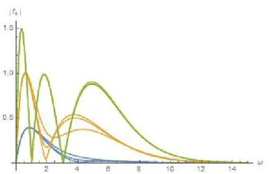
In the case of the trefoil-(2, 3)vortex knot, the amplitudes also contain a phase factor and in terms of spherical coordinates can be written as

f±(ω,θk,φk) =

(1±sgn(a))

2

√

πa2ω(1−cosθk)e−|a|ω ·(3−2|a|ω(1−cos(θk)) + 1

4a

2

ω2(1−cosθk)2

+ i

15|a|

3

ω3e−3iφksin3θk).

The corresponding spectrum, as depicted in Figure 3.3, is obtained by

plot-ting the modulus of the complex amplitude as function the frequency ω

while viewing it from different directions in Fourier space (different values ofθkandφk). We observe that although for small values of the polar angle

it is reminiscent to the Hopfion spectrum, it acquires a maximum of three peaks, asθkincreases. The effect of the azimuthal angle as it varies from 0

to 2πfor each value ofθk, is to modify the amplitude height and shape by

3.3 Invariants 23

Figure 3.3: Absolute value of the Fourier amplitude |f±|of the electromagnetic trefoil as function ofωfora = 1. The blue, orange and green colors correspond

to the values ofθ_k : 0.7, 1.4, 2.9radians, and within each color group (of constant θk) the different curves represent the values ofφk : 0.3, 1.5and1.9radians.

3.3

Invariants

To complete our investigation, we calculate the fundamental time

invari-ants of the Hopfion and the knotted vortex fields Fpq. Since we refer to

measurable quantities the material in this section is written explicitly in physical (SI system) units.

3.3.1

Helicity

An intriguing quantity that describes the topology of a field is known as the electromagnetic helicityh. It is associated with the topological concept of the winding number which was initially introduced by Gauss (1833) and over time has been attributed various interpretations; see Ref. [30] for a thorough historical review. For the Hopf field in particular, the helicity can be interpreted as an integer number times the index of the Hopf map (see page 5), which is a topological invariant [3]. The geometrical inter-pretation of the Hopf invariant is the linking (or winding) number of the

preimages of any two regular values of a map from S3 to S2 in the Hopf

3.3 Invariants 24

This interpretation of the helicity can be extended to the case of vor-tical fields. In analogy with the study of topological fluid dynamics, the electromagnetic field is viewed as being embedded in an incompressible, perfectly-conducting fluid (hydrodynamic approximation) carrying an iso-lated optical vortex loop with knotted structure. In this scheme, the value ofhdescribes the degree of knottedness or the “self-winding”∗of a vortex in the flow, multiplied by the square of its strength. With time evolution, the singular line is transported by a solenoidal velocity fieldu(r,t) (satisfy-ing∇ ·u =0)according to the “frozen field” equations ∂E

∂t =∇ ×(u×E), ∂B

∂t = ∇ ×(u×B), which govern its smooth deformation (no cutting or

gluing is allowed: the linkage is conserved) and consequently the helicity of the wave remains invariant.

The aforementioned topological constant, is expressed as the sum of the electric and magnetic helicities ash =he+hm and it can be defined in

terms of the electromagnetic potentialsC and Aby

h =

Z

d3r

e0

2 C·E+

1 2µ0

A·B

, (3.10)

the integral being over all space (for localized Maxwell solutions). It is noteworthy that, apart from the “frozen” fields case,his a constant of the motion also for electromagnetic waves satisfying the null property (requir-ing E·B = 0), as easily verified by taking the time derivative of Eq. 3.10 and using the relations in Eq. 2.3. Under certain conditions, the helicity coincides with its particle definition (the projection of the spin in the mo-mentum direction) describing thus the chirality or handedness of the flow, and it is also gauge invariant; for a systematic study of the properties ofh

see Refs. [28, 33]. In the Riemann-Silberstein notation and in terms of the

complex vector potentialV (Eq. 2.4) the helicity becomes

h = e0

2 Z

d3rF∗·V (3.11)

It should be noted that some authors prefer to include the square root of the factor e0

2 in the definition of F and V so that it would not appear

in this expression. In what follows, we omit writing it explicitly but for

∗_{This term was coined by Moffat [25], who has proposed a method to obtain the}

3.3 Invariants 25

dimensional consistency, it should multiply all the formulae that comprise the (absolute) square ofF or f±.

As demonstrated in the Appendix B, the helicity can be obtained via the complex amplitudes according to

h=

Z _d3_k

k (f

∗

+(k)f+(k)− f−∗(k)f−(k)). (3.12)

In the photon picture, the Fourier amplitudes can be replaced by the

quan-tum operators ˆf± =

√

¯

hcaˆ± and ˆf±∗ = √

¯

hcaˆ†±, where ˆa and ˆa† are the

creation and annihilation operators [9] and therefore Equation 3.12 can be interpreted (up to a scaling factor) as the classical limit for the difference between the number of right- and left- handed photons [33]. In the

fre-quency representation we can identify f± with the photon wave function

so that the Hopfion (a > 0), anti-Hopfion (a < 0) and all solutions built upon them describe photon states with positive and negative helicity, re-spectively.

3.3.2

Constants of the motion

Finally, we compute the dynamical quantities that govern the global

field-line evolution and are conserved with time. These are the energy E, the

linear momentum P, and the angular momentum J and can be expressed

in terms of the Riemann-Silberstein vector as

E=

Z

d3rF∗·F,

P= 1

ic

Z

d3rF∗×F,

J= 1

ic

Z

d3rr×(F∗×F). (3.13)

The linear and angular momentum densities are determined by the Poynt-ing vectorS = _µ1

0E×B = 1 2icµ0F

∗_{×F (divided byc}2_{)and guide the flow}

of energy. The velocity of this flow can be locally determined by the ra-tio of the momentum to the energy density and thus can be written us

u = c_iF_F∗∗×_·FF (cf. the relativistic formula reads |u| = c2|P_E|). By substituting

3.3 Invariants 26

E = 1

c

Z _d3_k

k ω(f

∗

+(k)f+(k) + f−∗(k)f−(k))

P = 1

c

Z _d3_k

k k(f

∗

+(k)f+(k) + f−∗(k)f−(k))

J = 1

c

∑

λ=±1 Z _d3_k

k f

∗

λ(k)(iDλ×k+λ

k

k)fλ(k) (3.14)

where

Dλ =∇k+λ

∑

e∗_j(k)∇_kej(k)).

The last expression in Equation 3.14 originates from quantum mechanics. In this framework the total angular momentum can be written as the sum of the spin and orbital operators acting on the photon states f±, with

z-component eigenvalues (`+σ)}. Here ` is the topological charge (see

Sec. 2.3) which describes the orbital angular momentum, and σ = ±1

represents the polarization of a photon which is associated with its spin. This reasoning, justifies the appearance of the 2 parenthesis terms and Dλ assumes the role of the covariant derivative (on the light cone) acting on

the k-dependent polarization vector∗. Note that this coincides with the

classical optics description within the paraxial approximation, where the total angular momentum can be expressed as the sum of spin and orbital contributions [23].

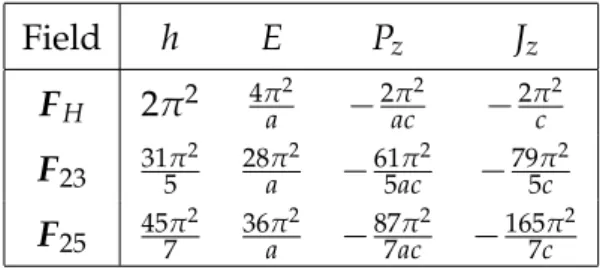
As an example, we present the calculated invariants for the Hopfion

FH, and two knotted vortex fields: the trefoil F23 and the cinquefoil F25.

For this we use the amplitudes f± as obtained in Subsection 20 and the

results are provided in Table 3.1. The values corresponding to FH are

in good agreement with the results suggested by Rañada [27]. The last 3 columns of the table indicate that the knotted vortex fields have finite energy which is moving along the z-direction while circulating about the

z-axis. Although we recognize a factor _p+q1 in the helicity, momentum and

angular momentum of the(p,q)-knotted vortex waves, their values do not in general follow a regular pattern as in the case of the fields 2.14; see Ref.

∗_{In Ref. [9] an extensive discussion on the analogy between quantum field theory and}

its classical counterpart in this context is provided. The particle interpretation, imposes a normalization condition on the photon states such thatf

ff2 ₌ R _d3_k

3.3 Invariants 27

[17]. At this point it is important to stress that the above results depend on the choice of coefficients in Equation 2.13 which will determine the exact shape of the knotted vortex.

Field h E Pz Jz

FH 2π2 4π

2

a −

2π2

ac −

2π2 c

F23 31π 2 5 28π

2

a −61π

2

5ac −79π

2 5c

F25 45π 2 7

36π2

a −

87π2

7ac − 165π2

7c

Table 3.1: The (non-normalized) values of the helicityh, energyEand the z com-ponents (which are the only non-vanishing) of the linear momentumPz and the

angular momentumJz. We usea >0and consider the case of the HopfionFHand

the fields with torus knot vorticesF23(trefoil) andF25(cinquefoil). As mentioned above, these values should be considered in units of e0

Chapter

4

Towards experimental realization

Optical vortices are ubiquitous in nature. Physical light, which can be de-scribed as a superposition of many plane waves traveling in different di-rections, delineates the perfect situation in which destructive interference can lead to the creation of threads of darkness. Interfering three or more plane waves can create a phase singularity in the laboratory [13]. In an optics experiment it is common to use laser beams as a light source, which are described by a Gaussian intensity profile and have well-behaved and understood properties. Among these are the well defined propagation direction and the high coherence of the output light. However, in con-trast with the broad spectral decomposition of the Hopfion and the torus knot vortex fields that we have studied (see Sec. 3.2), lasers are nearly monochromatic. This constitutes a major implication in the goal to realize them experimentally.

4.1

Spectral modification

To tackle this problem, we attempt to diminish the spectral width of our fields by modifying their Fourier amplitude. This is accomplished by mul-tiplying it with a scalar function of the frequency, or equivalently

(switch-ing back to natural units) the wavenumber k, which we denote as g(k).

This function is designed to have a narrow width while being peaked at a certain valuek0, such that to filter out only a few of the frequency

com-ponents of the original field. The resulting Fourier representation can be generically written as ˜F(k,t) = g(k)F(k,t). Under the constraints of being scalar and time-independent, an arbitrary choice for g(k) will serve for ˜F

nuga-4.1 Spectral modification 29

tory while F(k,t) is known to be a solution. This is made more intuitive by considering that (due to linearity) a single or a few components of a multi-colored superposition is still a Maxwell solution.

The spectral decomposition of the resulting field, in the form of Equa-tion 3.4, can be written as the the inverse Fourier transform

˜

F(r,t) =

Z _d3_k

(2π)3/2F(k,t)g(k)e

i(k·r−ωt)_{, (4.1)}

where for simplicity we have chosena>0. Apart from the 3-dimensionality of these integrals, polarization effects render their calculation long and te-dious. However, by expressing them in terms of spherical coordinates, we can exploit the fact that the spectra in Equation 3.7, contain a special combination of the frequency space coordinates which allows the angular part of each of the polarization components to be written as a finite sum of spherical harmonicsY_lm. Then, for a number of non-zero coefficients clm,

the jthcomponent can be written in the form

Fj(k,t) = ζ(k)

∑

l

∑

clmYlm(kˆ),

where ˆk stands for the Fourier angles (θk,φk) and ζ(k) contains the k

-dependent terms including the exponential factore−ik(t−i|a|). For instance, in the Hopfion case (Eq. 3.6) the functionζ takes the explicit formζ(k) =

a2√2π

4 ke

−ik(t−i|a|)_{and it is the same for all three components. As a common}

practice in momentum-space Feynman diagram analysis, we then replace the exponential factor in Eq. 4.1 with its Rayleigh expansion [2]

eik·r =

∞

∑

∑

4πiljl(kr)Ylm(rˆ)Y m∗

l (kˆ), (4.2)

where, as above, ˆr denotes the real space angles and jl is the spherical

Bessel function (of the first kind). Together with the orthonormality condi-tion for spherical harmonics which has the explicit formR dΩkYm

0

l0 (kˆ)Y m∗ l (kˆ) =

δll0_δmm0, wheredΩ_k = sinθ_kdθ_kdφ_kis the solid angle, the jthcomponent of

the integral 4.1 becomes

˜

Fj(r,t) =

∑

clmilYlm(ˆr)

Z

dkk2ζ(k)g(k)jl(kr). (4.3)

4.1 Spectral modification 30

due to the fact that the integrands contain a Bessel function together with an exponential, the solution is frequently inaccessible for a general g(k); for an extensive tabulation of Bessel integrals the reader is referred to [31].

There is one particular case for which the k-integral in equation 4.3

becomes trivial. This occurs for the choice of g(k) to be an 1-dimentional delta functionδ(k−k0), which corresponds to converting to the

monochro-matic variants of our fields at the frequency ω0 = k0. The resulting field

˜

F(r,t)essentially represents what we would “see” by looking at the(p,q)

knotted vortex fields through a single-colored glass. The explicit expres-sions (apart from the Hopf field case) resulting from this caclulation, are quite lengthy and therefore we shall not present them here. They are in-cluded in a Mathematica notebook which can be provided by the author on request.

Note that the Hopfion solution does not possess a vortex structure in its original form, and thus we do not expect that its single-colored variant would either. We therefore focus our attention to the case of the simplest torus knot vortex field, corresponding to the trefoil (2, 3). At zero time, several plots of planar intersections of the monochromatic field intensity (considering the electric and magnetic field vectors separately), exhibit in-teresting symmetries owing to its nature as superposition of Bessel func-tions. These plots contain multiple zero-intensity points which might in-stantly form a dark filament. Although a more careful investigation is re-quired to be able to draw a definite conclusion, at a first glance, the knotted vortex structure seems to not persist under the constraint of monochro-maticity. Moreover, the modified fields fail to satisfy the null condition and therefore, even if they did retain a topologically non-trivial structure att=0, it would be lost with time evolution.

A more systematic approach would involve imposing an external con-dition on the functiong(k), which will assure the nullness of the modified field, requiring

˜

F(r,t)·F˜(r,t) =

3

∑

j=1

˜

Fj(r,t)F˜j(r,t) = 0.

Using the fact that the Fourier transform of the product of two functions becomes the convolution integral of their individual Fourier transforms, the above condition, written in frequency space reads

3

∑

j=1

4.2 In a future laboratory 31

However, this expression involves 3-dimensional convolution integrals and therefore does not yield an obvious constraint on g(k) in order to be satisfied.

4.2

In a future laboratory

Due to the short time-span of this project and the aforementioned implica-tions, we unfortunately did not have the opportunity to directly engage in the practical aspects of knotting an electromagnetic vortex in the lab. Nev-ertheless, we devote this section to briefly outline and expose some ideas of how to make this experimentally feasible, assuming monochromaticity. In the laboratory, vortex carrying beams can be (readily) created be means of diffractive optical components. A high NA microscope objective lens can be used to create highly focused beams of light, from an arbitrary incident paraxial field. This was extensively studied by Leutenegger et al. [20], who proposed a numerical technique (fast Fourier transform) with which the amplitude, phase and polarization of the transmitted (focused) field can be fully determined via its plane wave spectrum.

Chapter

5

Conclusion

Optical fields with isolated (p,q) torus knot vortices exist as solutions to source-free Maxwell’s equations, and are endowed with special character-istic features; firstly due to the presence of the vortex itself, and secondly due to its non-trivial topology. Based on experimental interest, the main properties of these fields have been investigated to yield the following results. A transverse (to the vortex) saddle shaped polarization pattern occurs in the close vicinity of any vortex point in the field, while its orien-tation rotates as the reference point varies along the singular line. These results were verified in an analytical setting via dynamical systems the-ory. At the center of the saddle, a "new kind" of polarization singularity appears, and together with the observation that the spectra of these fields consist of a broad range of frequencies, this gives rise to a future research question: How can the study of polarization singularities be generalized to broad spectral fields and in what way does it relate to its monochro-matic analogue, on which previous literature is mainly focused? Further-more, because of the multi-colored spectra of these fields, a modification is necessary in order to accommodate the demands of a modern optics lab, in which any topological configuration of light could, in principle, be synthesized for a field consisting of one or just a few frequencies. It was shown that absolute monochromaticity is too strict to allow preservation of the vortex structure, and although a more appropriate (taking nullness into account) spectral modification might be promising, they are hard to deal with due to the laborious integral calculations that emerge.

Sec-33

tion 2.5. Thus, equipped with the suitable theoretical tools, the experi-mentalist is given the green light to go in the lab and attempt to twist and tangle the “darkness” of light into knots, complying our initial objective. Concluding, this issue certainly deserves further consideration from both the theoretical and experimental sides, since various research areas can benefit from the topological constraint of knottedness. In a more general view, the marriage between physics and the mathematical abstraction of topology reveals many fascinating future applications that are yet to be explored.

Acknowledgments

Appendix A: Computing the

Fourier transform

The analysis∗is greatly simplified by recognizing the patterned space-time coordinates appearing in the Hopfion (Equation 2.9) which are frequently encountered in the framework of general relativity and twistor theory [10]. For this reason, we introduce the (complex) space time variables

x± = x±iy, t± =t±z, τ± =t−ia±z

and denote the corresponding derivatives by ∇± = ∂

∂x± and ∂± =

∂ ∂t± =

∂

∂τ±. The scalar superpotential for the Hopfion (Equation 2.10) then

be-comes χ = 4a

2

x+x−−τ+τ−, providing a straight forward way to obtain the

expressionFH in Equation 2.9 according to

FH(r,t) = 1

2





−∇2 ++∂2+ −i(∇2

++∂2+) −2∇+∂+



χ(r,t). (A.1)

Employing a similar notation for the Fourier space coordinates: k± =kx±

iky, l± = ω ±kz, Equation A.1 enables the computation of the Fourier

decomposition of the Hopfion. This is achieved by writing χin it’s plane

wave expansion as

χ(r,t) =

Z _d3_k

(2π)3/2

2√2

ωl−

(f+(k)eiξ +f−∗(k)e−iξ), (A.2)

such that the derivatives only act on the exponentsξ = 1₂(k+x−+k−x+−

l+t−−l−t+) as written in terms of the new coordinates. This yields the

∗_{The material presented in this Appendix is based on an unpublished work by}

35

complex polarization vector

e(k) = 1

2√2ωl− 



k2−−l2−

i(k2−+l−2) −2k−l−



, (A.3)

which is normalized. The normalization condition justifies the appearance of the pre-factors in Equation A.2, which ascertain that the amplitudes f±

correspond to the specific choice ofe(k).

In order to generalize this result to(p,q)-knotted vortex fields as ob-tained by the summation in Eq. 2.13, we begin by calculating the spec-trum of the fields Frs = αrβsFH. This can be accomplished by expressing

the Bateman variables (Equations 2.8) in terms of the new coordinates as

α =1− 2iaτ−

x+x−−τ+τ−, β=

2ax−

x+x−−τ+τ−

Additionally, we introduce the new variableγ = 1−α so that the power

ofαinFrscan be replaced by the binomial expansion ofγsuch that

Frs(r,t) = r

∑

(−1)nβsγn

(x+x−−τ+τ−) 



−β2−γ2

−i(β2−γ2)

−2iβγ 

. (A.4)

Again, due to the elegant choice of space-time coordinates which provide the following useful identity

βrγs

x+x−−τ+τ− =

(2ax−)r(2iaτ−)s

(x+x−−τ+τ−)r+s+1

= (−2a)

r_(2ia)s

4a2_(r+s)! ∇ r +∂s+χ,

we can replace the powers of the Bateman variables with the rth and sth

derivatives of the superpotential.This maneuver enables us to obtain the plane wave decomposition of Equation A.4 in a similar manner as in the Hopfion case above (including these derivatives in each component). For a choice of non-zero coefficientsλrs and due to the linearity of the Fourier