MODELING LONGITUDINAL MEDIATION OF WITHIN-PERSON CHANGES
Corinne M. Henk
A thesis submitted to the faculty of the University of North Carolina at Chapel Hill in partial fulfillment of the requirements for the degree of Master of Arts in the Department of Psychology.
Chapel Hill 2016
Approved by:
Laura Castro-Schilo
Daniel J. Bauer
ABSTRACT
Corinne M. Henk: Longitudinal Mediation of Within-Person Changes (Under the direction of Laura Castro-Schilo)
Mediation analysis concerns the discovery of mechanisms that transmit an effect from
one variable to another. At times, social scientists propose hypotheses involving mediation of
within-person changes (e.g., do within-person changes in cognitive ability mediate the relation
between changes in depression and changes in disability?) The current manuscript introduces an
approach within the latent change score (LCS) modeling framework to test such hypotheses. This
approach is compared to existing methods, including the cross-lagged panel model (CLPM; Cole
& Maxwell, 2003) and the LCS mediation model (Selig & Preacher, 2009). Results from (1) a
single-replication simulation and (2) an empirical example utilizing data from the Health and
TABLE OF CONTENTS
LIST OF TABLES……….……….………....vi
LIST OF FIGURES……….……….……….vii
CHAPTER 1: INTRODUCTION……….………...1
The Cross-Lagged Panel Model……….………..5
Advantages of the CLPM……….………..……..8
The Latent Change Score Mediation Model……….……….………....13
The Cross-Lagged Latent Change Score Model……….…………...…17
Relations Among Structural Parameters in the CLPM and CL-LCS Model……….20
Limitations of the CLPM.……….……….21
CHAPTER 2: METHOD……….………..23
Proof of Concept……….……….……...23
Participants and Procedures……….………..24
Measures……….………...25
Data Analysis……….………....27
CHAPTER 3: RESULTS……….………...….30
Proof of Concept……….………...30
Illustration: Descriptive Statistics……….……….31
Illustration: CL-LCS Model Results……….……….32
APPENDIX A: R CODE FOR SIMULATING CL-LCS DATA……….58
APPENDIX B: EXAMPLE MPLUS CODE FOR FITTING CL-LCS MODEL….…………....62 ENDNOTES……….……….………65
LIST OF TABLES
Table 1. Unstandardized Results: CL-LCS Model, No Linear Trend Simulation……….40
Table 2. Unstandardized Results: CL-LCS Model, Linear Trend Simulation………...42
Table 3. Descriptive Statistics: Indicators of Depression, Cognitive Ability, and Disability...…44
LIST OF FIGURES
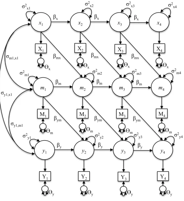
Figure 1. Path diagram of one specification of Cole and Maxwell’s (2003)
CLPM with latent variables.……….……….47
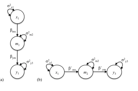
Figure 2(a). Causal steps cross-sectional model. .……….………48
Figure 2(b). Causal steps model with temporal separation……….………...…………48
Figure 3(a). Basic LCS building block with the initial level-to-change association
specified as a regression……….……….………..….49
Figure 3(b). Basic LCS building block with the initial level-to-change association
specified as a correlation. .……….………....49
Figure 4. Path diagram of Selig and Preacher’s (2009) LCS-MM………50
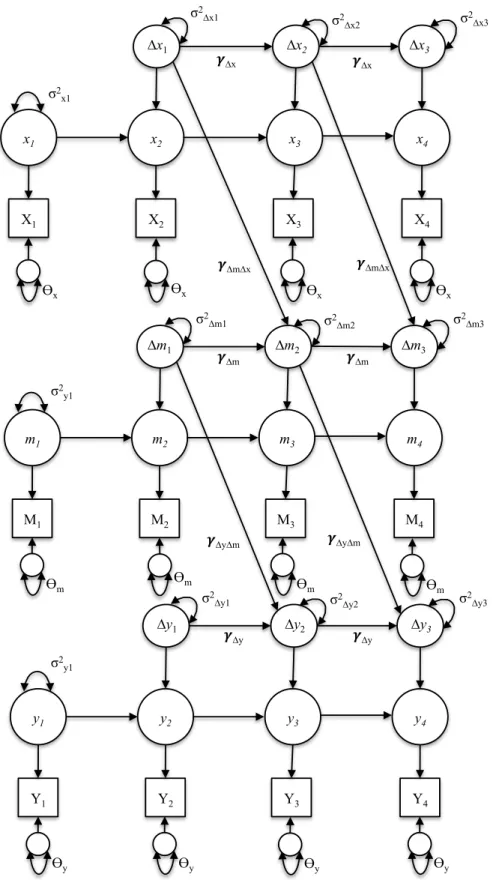
Figure 5. Path diagram of a fully mediated process using the CL-LCS………51
Figure 6. Conceptual diagram of the CL-LCS in the case of full mediation….………52
Figure 7. Random selection of 100 simulated trajectories governed by
no trend across 4 waves……….53
Figure 8. Random selection of 100 simulated trajectories governed by a linear trend
across 4 waves. .……….……… .……….………….54
Figure 9. Individual trajectories of a random sample of 100 HRS participants’
factor scores on depression over time. .……….…..……… ……….55
Figure 10. Individual trajectories of a random sample of 100 HRS participants’
factor scores on cognitive ability over time. ……….………56
Figure 11. Individual trajectories of a random sample of 100 HRS participants’
CHAPTER 1: INTRODUCTION
Mediation analyses are ubiquitous in the social sciences; at the time of writing, the term
mediation generated 1.43 million results in a Google scholar search. Increasingly, psychologists seek to understand not just whether two constructs are related, but why the relation exists. While cross-sectional data were once considered sufficient for conducting sound mediation analyses,
researchers now recognize that longitudinal data are preferable for gleaning insight into
unfolding mediation processes. Indeed, repeated measures afford researchers the opportunity to
draw stronger inferences about the nature of relations over time (e.g., Shadish, Cook, &
Campbell, 2002).
When working with longitudinal data, hypotheses about change predicting future change
often emerge (Baltes & Nesselroade, 1979). As an example, researchers hypothesize that
increases in lateral ventricle size predict subsequent declines in memory performance among older adults (Grimm, An, McArdle, Zonderman, & Resnick, 2012). Research questions involving
associations among changes are central to longitudinal research; in fact, Grimm and colleagues
(2012, p. 268) posit that a key goal of developmental science is to “[understand] the dynamic
interplay between two (or more) constantly changing constructs.” Hypotheses involving
change—as a predictor, mediator, and/or outcome—are becoming more common in
psychological research. Indeed, researchers interested in modeling change as both a predictor and
an outcome will find that the “change-to-change” literature is expanding (e.g., Grimm et al.,
Importantly, these change-to-change hypotheses are qualitatively and quantitatively
distinct from other types of research questions, such as those that involve the level or status on a
variable as a predictor of change in another variable (i.e., level-to-change hypotheses). To clarify
the qualitative differences, consider two examples. First, a level-to-change hypothesis may posit
that older adults with the highest levels of depression will show the most declines in cognitive ability later in life. In contrast, a change-to-change hypothesis may be that as individuals become
more depressed (increase on depression), they will show either gains or less rapid declines in cognitive ability. In this case, change is the mechanism by which the relation operates. One does
not have to search far and wide in psychology to find unique examples of level-to-change and
change-to-change hypotheses. Each type of hypothesis demands a quantitative strategy that will
appropriately test the associations of interest, yet strategizing is not always straightforward.
Compounding the task of selecting an optimal modeling strategy is the issue of whether
the motivating hypothesis entails tests of within-person effects, between-person effects, or both
(e.g., Curran & Bauer, 2011). Somewhat vexingly, level-to-change and change-to-change
hypotheses can be focused on any combination of within- or between-person associations. A
researcher’s analytic choices determine which types of effects are tested. For example, consider
again the level-to-change hypothesis that individuals who are more depressed have more drastic
declines in cognitive ability. If interest lies in the between-person effect, one appropriate
modeling strategy could be to use a parallel process latent growth model (Cheong, MacKinnon,
& Khoo, 2003), with the intercept of depression predicting the slope of cognitive ability.
Similarly, if interest lies in the between-person effect when considering the change-to-change
hypothesis that changes in depression are linked to changes in cognitive ability, a parallel
means of the slopes to aid interpretation, a researcher could conclude that on average, increases
in depression are associated with decreases in cognitive ability (assuming the means were
positive and negative for depression and cognitive ability, respectively). Results would inform
the degree to which relations held between-persons.
However, when interest lies in within-person change-to-change effects, a correlation or
regression among parallel process slopes will not be informative, and it becomes necessary to
consider alternate modeling strategies. Researchers may formulate a within-person
change-to-change research question to understand, for example, whether a particular individual who has
decreasing severity of depression will subsequently experience changes in her cognitive ability.
These hypotheses have major implications and ramifications for individual-targeted interventions
and individualized medicine, where interest lies in whether changes in one variable will produce
changes in another variable at the individual level. A key goal of the current work is to clarify best practices for testing hypotheses regarding within-person change-to-change relations, as
these types of hypotheses have received relatively little attention in the quantitative psychology
literature.
Although many mediation hypotheses fundamentally posit within-person change as a
predictor and an outcome, the most common approach for testing longitudinal mediation—the
cross-lagged panel model (CLPM; Cole & Maxwell, 2003)—focuses on within-person
level-to-change associations (Preacher, 2015). Unfortunately, within-person level-to-change-to-level-to-change
hypotheses cannot be tested using the CLPM, as this model can only accommodate change as an
outcome—not as a predictor. Testing within-person change-to-change hypotheses requires
explicit specification of change in statistical models. Belonging to the structural equation
patterns, causes, and consequences of intraindividual change (e.g., Castro-Schilo, Ferrer,
Hernández, & Conger, 2015; Ferrer & McArdle, 2010; Grimm, Castro-Schilo, & Davoudzadeh,
2013; McArdle, 1994; McArdle, 2001; McArdle, 2009; McArdle & Hamagami, 2001, McArdle
& Nesselroade, 1994). In this framework, within-person changes are explicitly represented as
latent variables, a feature that enables change to be specified as a predictor, criterion, or both.
Selig and Preacher (2009) capitalized on the LCS framework and introduced the LCS mediation
model (LCS-MM) for testing mediational hypotheses rooted in within-person changes. However,
a major setback of the LCS-MM is that its setup precludes testing competing patterns of
causality.
To illustrate this point and to foreshadow an empirical example that will be presented
later in this project, consider a hypothesis positing that for an aging adult, the relation between
his/her changes in depression (X) and changes in disability (Y) is mediated by changes in
cognitive ability (M). A competing causal hypothesis would consist of switching the roles of
these variables, treating changes in disability as the exogenous predictor (X) and changes in
depression as the outcome (Y), yet testing this hypothesis with the LCS-MM would result in two
non-nested models that are not easily comparable. Another competing hypothesis could include
bidirectional effects (e.g., changes in depression and changes in disability having reciprocal
relations)—but such effects cannot be specified in the LCS-MM. As such, researchers relying on
the LCS-MM may inadvertently engage in confirmation bias because this approach is designed
to test only the a priori hypothesis. Thus, the goal of this project is to introduce a model, which I
term the cross-lagged LCS (CL-LCS) model, that allows for more rigorous tests of within-person
change-to-change mediation.
and explicate its key advantages relative to cross-sectional approaches to assessing mediation. I
then present the LCS-MM and CL-LCS models, and compare their appropriateness for assessing
longitudinal mediation among intraindividual changes. I show analytically that results and
significance tests from the CL-LCS model will necessarily differ from the CLPM approach. I
also enumerate some of the limitations of the CLPM approach and provide further rationale for
using the CL-LCS model in applications in which data exhibit systematic mean changes over
time. Next, I present a small simulation study as a proof of concept; that is, when data are
generated to follow a CL-LCS process, the model appears identified and can be estimated with
reasonable parameter estimates. Then, using an empirical example of data from the Health and
Retirement Study (HRS), I fit the CL-LCS model to test the hypothesis that within-person
changes in depression lead to changes in cognitive ability, which in turn lead to changes in
disability. Henk and Castro-Schilo (2015) found support for this hypothesis using just two waves
of data; here I test the hypothesis using four waves of data, which provides potential for stronger
internal validity. I conclude by enumerating strengths and limitations of the suggested CL-LCS
approach and provide future directions for research on this newly developed model.
The Cross-Lagged Panel Model
The CLPM can be specified with observed or latent variables in the SEM framework;
here, I consider the latter as doing so will facilitate discussion of other models that rely on latent
variables. Figure 1 depicts a specification of the CLPM with three constructs, x, m, and y. For simplicity, each construct is measured with just one indicator across four time-points (i.e., X1, …
X4, M1… M4, Y1…Y4), although multiple-indicators could be included to define common
factors.
fixing factor loadings to 1, such that measurement error can be estimated and parsed from true
score variability (Jöreskog, 1978),
Xit = xit + δxit (1)
xit = Xit – δxit (2)
where Xit is the observed variable for individual i at time t, xit is the latent true score for
individual i at time t, and δxit is the measurement error for individual i at time t and is ~N(0, θx)
and assumed to be uncorrelated with Xit. For identification, these error variances are fixed to equality across time (although with enough waves of data, some equality constraints in error
variances may be relaxed; see Jöreskog, 1978). Equations (1) and (2) operate identically for the
m and y process. The latent variables at the first wave of assessment are exogenous and freely allowed to correlate. All other latent variables (i.e., after Wave 1) are described by an
autoregressive (AR) process such that a given variable is a function of its true score at the
previous time-point, plus a disturbance:
xit = βx (xit-1) + ξxit for t > 1 (3)
where βx is the AR parameter quantifying the rank-order stability over time for xit, xit-1 is
individual i’s latent factor score at the previous point in time, and ξxit is a time-specific residual
assumed to be ~N(0, Θx) and uncorrelated with the initial score xit-1, and all other terms are as
defined above. In Figure 1, the m process is defined to be a function of itself and x at the prior time-point,
mit = βm (mit-1) + βmx (xit-1) + ξmit for t > 1 (4)
where βm is the AR parameter, mit-1 is individual i’s latent factor score at the previous point in
time, βmx is the cross-lagged effect capturing the effect of x on m, and ξmit is a time-specific
Similarly, the y process is governed by an AR and cross-lagged process:
yit = βy (yit-1) + βym (mit-1) + ξyit for t > 1 (5)
where βy is the AR parameter, yit-1 is individual i’s latent factor score at the previous point in
time, βym is the cross-lagged parameter, and ξyit is a time-specific residual assumed to be ~N(0,
Θy) and uncorrelated with the initial score yit-1, mit-1, and xit-1. All other terms are as defined
above. Importantly, Figure 1 represents just one potential specification of the CLPM; other
specifications are important for systematic assessment of mediation, such as the inclusion of
direct effects from x to y, bidirectional effects, or competing models of causality (e.g., y predicts
m, which predicts x). Moreover, it is worth noting that Equations 3-5 do not include an intercept because the CLPM assumes data are centered; that is, no stable between-person differences exist
(Hamaker, Kuiper, & Grasman, 2015).
Interpretation of the AR parameters (e.g., βx and βy in Figure 1) is straightforward; these
represent rank-order stability in the construct over time. An AR coefficient of 1 indicates the
construct under study is perfectly stable over time. Here, the term stable refers to a lack of interindividual differences in within-person change; either no one is changing, or every
individual experiences the same amount of change with respect to magnitude and direction. An
AR parameter estimated at 1 suggests the rank ordering of individuals remains unchanged over
time (e.g., Person A has the highest depression at all waves of assessment; Person B has the
lowest scores on depression at all waves of assessment), assuming the disturbances do not
disrupt the rankings. Generally, however, AR coefficients are estimated at some value less than
1.
The cross-lagged coefficients (e.g., βmx andβym in Figure 1), also called coupling
expected shift in yit given a 1-unit increase in mit-1, controlling for the prior level of y (i.e., yit-1). Because the effect of yi1 on yi2 is partialed out, the coupling parameter can be interpreted as a
prediction of change in y. Thus, the CLPM is equipped to model change as an outcome, but not as a predictor. At best, relations among changes in different constructs can be captured in the
CLPM through estimation of within-time correlations among residual variances, although this
specification would not be informative of structured (e.g., lead-lag) relations among changes. In
sum, specification of the CLPM is most informative for hypotheses about lead-lag relations
among the level (or status) of variables, but cannot speak to change-to-change hypotheses.
Advantages of the CLPM
The CLPM is widely used for evaluating longitudinal mediation in the social sciences;
according to a Google Scholar search, it had been cited over 1,200 times at the time of writing
this paper. Given that this model was explicitly developed to address shortcomings of the
cross-sectional causal steps approach (Baron & Kenny, 1986), a brief description of that model
follows. Then, the advantages of the CLPM are discussed in detail.
The causal steps approach involves testing three regression models: (1) the regression of
the dependent variable (Y) on the independent variable (X)1; (2) the regression of the mediator (M) on X; and (3) the multiple regression of Y on both X and M. If a mediation process is
underway, the first two models will yield significant regression coefficients, signaling that X has
a direct effect on Y, and that X has a direct effect on M. Moreover, the effect of X on Y should
diminish once the effect of M is accounted for (i.e., when comparing the relevant coefficients
from the first and third regression models); this is termed partial mediation. In the case of full
mediation, the effect of X on Y will drop to zero when M is accounted for.
among variables. However, Sobel (1990) argued that for true mediation to hold, M “must truly
be a dependent variable relative to X, which implies that X must precede [M] in time; and [M]
must be a truly independent variable relative to Y, implying that [M] precedes Y in time” (Cole
& Maxwell, 2003, p. 561). As such, researchers have emphasized the importance of using
longitudinal data to conduct more rigorous tests of mediation. Indeed, Cole and Maxwell (2003)
made a critical contribution to this literature when they expanded the causal steps approach with
the cross-lagged panel model (CLPM), which can accommodate tests of longitudinal mediation.
There are four key advantages of the CLPM as compared to the causal steps approach. (1)
Accounting for prior values of endogenous variables leads to unbiased estimates of cross-lagged
effects. (2) The CLPM allows estimation and testing of overall indirect effects. (3) Alternate
lagged effects may be tested. (4) Alternate models of causal direction can be tested (e.g., perhaps
Y has an effect on X that is mediated by M, rather than X affecting Y through M). In this section,
I will explain each of these advantages in detail.
The key difference between the CLPM and Baron and Kenny’s (1986) causal steps
approach of testing mediation is that the former accounts for prior values of each endogenous
variable. Cole and Maxwell (2003, p. 560) call these prior values an “almost ubiquitous third
variable confound” because, as is well known within the context of the general linear modeling
(GLM) framework, regression coefficients will be biased if important predictors are omitted
from the model. The reason is that these coefficients are partial regression weights; thus, their
values change depending on the other predictors in the model and the degree to which those
predictors correlate (i.e., share variance) with each other. Two variables measured at the same
time-point (e.g., X1 and M1) are likely to be correlated, if for no other reason than by virtue of
effect of X1 to M2, M1 must be included as a covariate. Failing to control for prior values of an
endogenous variable—as in the causal steps approach—will almost always lead to inflated
estimates of the direct and indirect effects. Figure 2 displays two models that could be assessed
with the causal steps approach for testing mediation: (a) a cross-sectional mediation model and
(b) a mediation model with temporal separation. Notably, although Figure 2b incorporates
longitudinal data, it too will lead to biased estimates of β’
mx and β’ym. Temporal separation of
the independent variable, mediator, and outcome is not sufficient for obtaining accurate
coefficients; it is critical to control for prior values of each endogenous variable (Cole &
Maxwell, 2003).
In addition to controlling for prior values of endogenous variables—thus yielding more
accurate estimates—the CLPM includes a simultaneous test of overall indirect effects, whereas
the causal steps approach tests each time-specific indirect effect. The overall indirect effect
captures the total extent to which the independent variable transmits an effect on the outcome
through the mediator, across the entire duration of the study. Consider the specification of Figure
1. The overall indirect effect that x has on y is equal to the sum of all indirect effects across waves:
(a) x1à x2à m3à y4 = (βx • βmx • βym)
(b) x1à m2à m3à y4 = (βmx • βm • βym)
(c) x1à m2 à y3à y4 = (βmx • βym • βy)
Overall Indirect Effect = βx • βmx • βym + βmx • βm • βym + βmx • βym • βy
= βmx(βx • βym + βm • βym + βym • βy)
= βmx(βym(βx + βm + βy)) (6)
point is particularly important because mediation is usually conceived of as an ongoing,
unfolding process as opposed to a one-time occurrence; thus, differentiating time-specific
indirect effects from the overall indirect effect is key (Cole & Maxwell, 2003). Moreover, if a
researcher has gone through the process of collecting longitudinal data, it behooves him or her to
make full use of every wave of data. Ultimately, more waves of data provide a more accurate
estimate of the overall indirect effect.
The third advantage of the CLPM is that it allows for tests of alternate autoregressive
relations. Figures 1 and 2 only have lag-1 relations (i.e., each construct is predicted by itself at
the prior time-point), but in some research settings it may be appropriate to include lag-2 paths.
Cole and Maxwell (2003, p. 571) suggest that these “wave-skipping paths” may indicate
“interesting nonlinear relations: The system may not be stationary, causal relations may be
accelerating or decelerating, or the selected time lag between waves might not be optimal to
represent the full causal effect of one variable on another.” Testing the need for additional lagged
effects can be done using a series of likelihood ratio tests (LRT) as the reduced set (e.g., lag-1) is
nested within the larger model. If there is a significant increment in fit when additional lags are
included, these paths should be retained.
Lastly, and perhaps most importantly, the CLPM allows for tests of alternate patterns of
causality, which is a critically important step in SEM underscored by MacCallum, Wegender,
Uchino, and Fabrigar (1993). In their seminal paper, the notion of equivalent models was
introduced. That is, there may exist alternative models that are mathematically equivalent (i.e.,
provide identical model fit) to the proposed/hypothesized model. The authors conducted a
literature review and showed that many applications of SEM neglect to consider alternate,
alone many) equivalent models presents a serious challenge to the inferences typically made by
researchers using [SEM]” (p. 196). Potential solutions of this serious issue include
experimentally manipulating key variables and/or using longitudinal designs. Both of these
approaches allow researchers to safely rule out at least some alternative models. In the case of
longitudinal designs, equivalent models that involve effects moving backward in time (e.g., X at
Time 2 predicting M at Time 1) are not plausible and can thus be ruled out.
Most applications of the causal steps approach involve testing mediation with
cross-sectional data (see Figure 2a), which precludes testing the directionality of effects. Theory may
suggest a model wherein x predicts m, which then predicts y, but the “true” model may be such that y is exogenous with respect to m, and m is exogenous with respect to x. These two models are indistinguishable using the causal steps method,3 but can be tested in the CLPM. Namely, LRTs can be conducted to distinguish the directionality of effects based on model fit. A full
CLPM can be specified to include bidirectional effects, such that (a) x predicts m, which predicts
y, and (b) y predicts m, which predicts x. Removing paths in part (a) or (b) allows for LRTs; if significant, the LRT suggests the fit of the model significantly worsens with the removal of these
paths, and thus relevant effects should be retained in the model. Even in longitudinal applications
of the causal steps approach, however, testing alternate patterns of causality is not
straightforward, as each construct is represented at one and only one point in time (see Figure
2b). Thus, respecifying the model to test an alternate causal process (e.g., Y predicting M,
predicting X) requires a different set of data wherein Y is measured at Time 1, M at Time 2, and
X at Time 3.
Recall the motivating hypothesis that the relation between changes in depression and
possibilities: equivalent models (i.e., that provide identical model fit) and alternate models that
posit a different structure of causality but do not provide identical fit (i.e., Y predicts M, which
predicts X, instead of the a priori hypothesis that X leads to M, which leads to Y). Fitting the
CLPM is not a panacea for the problem of equivalent models; equivalent models will still be
present. However, the setup of this model does allow researchers to test alternate structures of
causality. In fact, Cole and Maxwell (2003) encouraged researchers to evaluate the tenability of
different models of causality, and termed the pathways in these alternative models “theoretically
backward effects.” To avoid confusion with backward-in-time effects, I use the term “alternative
models of causality.” Ultimately, testing alternative models of causality helps researchers to
avoid engaging in confirmation bias. To the extent that one alternate model of causality provides
better fit to the data than the a priori model—and makes sense from a theoretical standpoint—it
may be warranted to conduct future studies and/or revise the original hypothesis.
In sum, the CLPM offers many advantages over the traditional causal steps approach, and
is held in high esteem for this reason. However, when a researcher’s motivating theory includes
within-person change as a predictor of subsequent change, it is necessary to move to an alternate
framework.
The Latent Change Score Mediation Model
The LCS framework affords great flexibility in using intraindividual change as an
outcome, predictor, or both. Before delving into the LCS-MM, I begin by presenting some basic
latent change score concepts. First, to specify a latent change score, “true” scores are separated
from their imperfectly measured observed variable counterparts, exactly as was done in
Equations (1) and (2). Then, as implied in the following equation,
creation of latent change scores relies on the imposition of unit-weighted autoregressive effects,
which imply that a latent score (i.e., level) at time t is exactly equal to itself at time t – 1plus the change that occurred between time t – 1 and t. (Note that the subscripts of the change scores begin at 2 because at least two waves of data must be collected before changes can be modeled).
Contrast this expression with that of Equation (3), which expresses the “level” equation for x in the CLPM. At first glance, the LCS formulation may appear to be a subset of the CLPM with the
autoregressive effect fixed to 1, yet these models are not nested. The “residual” in the LCS
framework is the within-person change (Δxit) and is allowed to correlate with or be regressed on xit. The rationale for estimating this correlation/regression is that in many research contexts, initial levels of a construct are associated with how much change takes place. In contrast, the
residual in the CLPM (and in any traditional regression model)—by definition—is assumed to
have zero correlation with the predictors (see Figure 3 for a path diagram of the latent change
score basic building block that maps onto Equation 6).
Importantly, the imposition of perfect autoregressive effects allows for the explicit
representation of within-person change as a latent variable, which lends itself to testing different
structural relations among the changes. Indeed, a variety of structures can be imposed on the
latent change scores (see McArdle, 2009 for a description of common LCS model
specifications). Most LCS specifications include level-to-change predictive paths, within- and
across-constructs. To my knowledge, Selig and Preacher (2009) introduced the first
change-to-change specification with the LCS-MM, although others had been exploring change-to-change-to-change-to-change
models in substantive fields prior to that (e.g., Hertzog et al., 2003).
A path diagram of the LCS-MM is displayed in Figure 4. To achieve temporal separation,
time-points such that x is modeled only at Time 1 and 2, m is modeled at Time 2 and 3, and y is modeled at Time 3 and 4. I uphold this convention for clarity, although the spacing of
assessments could vary in practice. Because the latent changes are the outcomes of primary
interest, I present these equations below:
∆xi2 = βx (xi1) + ξ∆xi2 (8) ∆mi3 = βm (mi2) + βmx (xi1) + β∆m∆x (∆xi2) + ξ∆mi3 (9) ∆yi4 = βy (yi3) + βym (mi2) + βyx (xi1) + β∆y∆m (∆mi3)
+ β∆y∆x (∆xi2) + ξ∆mi4 (10)
In the LCS-MM, changes in x in the first interval (∆xi2) for person i are a function only of the
initial level of x plus a disturbance, ξ∆xi2. Changes in m are modeled in the second interval (∆mi3),
and are structured as a function of the level of m at Time 2, the level of x at Time 1, the change in x between Time 1 and 2, and a disturbance ξ∆mi3. Finally, changes in y are modeled in the third
interval (∆yi4), and are a function of the level of y at Time 3, the level of m at Time 2, the level of x at Time 1, changes in m that occurred between Time 2 and 3, changes in x that occurred
between Time 1 and 2, and a disturbance ξ∆yi4.
When comparing aspects of the LCS-MM to the standards put forth by Cole and Maxwell
(2003), there are several discrepancies worth noting. First, Cole and Maxwell (2003) established
the need to control for prior values of endogenous variables through use of autoregressive
effects. In the LCS-MM, interest primarily lies in the cross-construct change-to-change effects,
which suggests that within-construct prior changes should be accounted for. Stated differently, if a researcher is interested in predicting changes in m between Time 2 and 3 from changes in x
between Time 1 and 2, an unbiased estimate of this effect will only be obtained if the effect of
interval (i.e., between Time 1 and 2), it is likely that changes in x and changes in m will be correlated; thus, it is requisite to include prior changes in m as a predictor. However, given that the LCS-MM has only one change score per construct, this specification is not possible.
Importantly, the LCS-MM does control for prior levels of x, m, and y. Consider again the case in which the motivating hypothesis is that changes in x (∆x) predict changes in m (∆m), which subsequently predict changes in y (∆y). The partial regression weights β∆m∆x and β∆y∆m will
inform this hypothesis. Namely, β∆m∆x will represent the effect ∆x has on ∆m, accounting for prior levels of m. Whether prior levels shouldbe controlled for is the concern of Lord’s Paradox (Lord, 1967). Lord’s Paradox was introduced in the context of an experimental design with two
groups. The paradox refers to the fact that researchers draw discrepant results and conclusions
depending on whether they (a) use the grouping variable (i.e., control versus experimental) to
predict the Time 2 post-test, while controlling for the Time 1 pre-test (e.g., in an ANCOVA), or
(b) predict change (i.e., Time 2 post-test minus Time 1 pre-test) from the grouping variable (e.g.,
in a difference/change score model). Recent work has explored the issue of Lord’s Paradox and
clarified a number of aspects: (1) it is not limited to experimental designs with a categorical
grouping variable, but rather pertains in the context of a continuous predictor as well; (2)
ANCOVA and difference/change models make different assumptions about the data, and these
assumptions are untestable; and (3) difference/change score models are preferable over
ANCOVA models in the context of observational studies, whereas ANCOVA is preferable when
randomization is part of the study design (van Breukelen, 2013; Castro-Schilo & Grimm, in
press). Analogous to ANCOVA, the LCS-MM controls for previous levels of x, m, and y, but this practice might only be ideal in experimental studies. Instead, controlling for prior changes in x,
There is another aspect of the LCS-MM that will be troublesome in most if not all
applications. First, recall that one of the benefits of the CLPM is the ability to test alternate
structural relations among processes (e.g., lag-2). Unfortunately, the variety of structures that can
be tested using the LCS-MM is limited by the fact that there is just one change score per
construct. As a result, this setup prohibits testing different autoregressive structures among the
changes. Similarly, it is not possible to test different patterns of causality (e.g., ∆y predicting ∆m, predicting ∆x) in the LCS-MM because each downstream latent change is modeled at a later point in time than the upstream change scores. In the context of the depression, cognitive ability,
and disability hypothesis, the LCS-MM would require changes in depression to be modeled
between Time 1 and 2, changes in cognitive health between Time 2 and 3, and changes in
depression between Time 3 and 4. Thus, it would be impossible to test a model wherein changes
in disability lead to changes in cognitive health, which then lead to changes in depression. Such a
model would test temporally backward effects, unless a different set of data was used. Thus, the
setup of the LCS-MM may lead researchers to engage in confirmation bias with increased
frequency. This unfortunate consequence of the LCS-MM is the major impetus for the
development of an expanded LCS model suited for testing mediation among changes.
The Cross-Lagged Latent Change Score Model
At each time-point and for each construct, the measurement model of the CL-LCS model
is expressed as in Equation (1). For maximum benefits, each level/status of the constructs across
time should be modeled as multiple indicator latent factors so that the factors capture common
variance and can be purged from measurement error. However, for simplicity I consider the case
of only one indicator per construct, fixing the residuals of the manifest variables to equality as
residuals of the indicators) is preferable over taking the differences of observed variables
because the factors are corrected for unreliability of the manifest variables. Moreover, a
fundamental advantage of the LCS modeling framework is to be able to purge difference/change
scores from measurement error, as traditional criticisms of difference/change scores no longer
apply when these are perfectly reliable (Schilo & Grimm, under review; Henk &
Castro-Schilo, 2015).
For the structural specification of the CL-LCS model, each process has two exogenous
variables: the initial level (i.e., at Time 1) and the first latent change score. After the first
time-point, the level for each construct is defined as a function of the previous time-point plus the
within-person change, exactly as was done in Equation (6).
The hallmark of the CL-LCS model is its ability to flexibly incorporate various structural
associations among the change scores. Here, I consider one potential specification; that is, the
case whereby the effect that ∆x has on ∆y is fully mediated through ∆m (see Figure 5). For the x
process, each change score after the first interval is specified as a function of the prior change
score:
Δxit = γ∆x (∆xit-1)+ ζ∆xit for t > 1 (11)
where Δxit is the latent change that occurred between time t – 1 and t, γ∆x is the autoproportion
effect capturing the influence of prior change on current change, ∆xit-1 is the prior change in x, and ζ∆xit is a random disturbance for individual i at time t. In this specification, I set γ∆x to be
invariant across time, although this assumption may be relaxed. The m and y processes operate similarly, except each has an additional term in its equation to capture the cross-construct
change-to-change effects:
Δyit = γ∆y (∆yit-1)+ γ∆y∆m (Δmit-1)+ ζ∆yit for t > 1 (13)
where γ∆m∆x is the change-to-change effect of prior ∆xiton Δmit, ζ∆xit is a random disturbance for
individual i at time t, γ∆y∆m is the change-to-change effect of ∆m at the previous time-point on
∆y, and ζ∆yit is a random disturbance for individual i at time t. All disturbances are uncorrelated
with one another and with all other latent variables in the model. However, this assumption can
be relaxed to accommodate within-time covariances among the residuals of the change scores.
Incorporation of these covariances implies there are omitted causal effects that explain shared
residual variance in the change scores. Notice that unlike Equations (8) and (9), the change score
equations here do not include levels as predictors.
In many ways, the CL-LCS model can be considered an extension of the LCS-MM.
Specifically, the CL-LCS expands upon the LCS-MM so that changes in each construct can be
modeled at every time-point, rather than only at pre-selected waves. Contrast Figure 5, which
contains a path diagram of the CL-LCS model, with Figure 4; with four time-points of data, the
CL-LCS model contains nine latent change score variables—three per construct—as opposed to
the LCS-MM, which includes just one latent change per construct. Importantly, inclusion of
multiple latent changes for each construct in the CL-LCS model allows researchers to conduct
more rigorous tests of longitudinal mediation (Cole & Maxwell, 2003).
In sum, the CL-LCS model specification has several key advantages over the LCS-MM
approach. The CL-LCS controls for prior values of each endogenous latent change, which yields
unbiased cross-construct change-to-change effects. Moreover, the CL-LCS allows for tests of
overall change-to-change indirect effects (provided there are four or more waves of data),
whereas the LCS-MM allows for tests of overall indirect effects, but the change-to-change
between Time 2 and 3, changes in y between Time 3 and 4). Finally, the CL-LCS allows
researchers to test different structures of causality. A full CL-LCS model can be specified so that
(a) changes in x predict changes in m, which predict changes in y and (b) changes in y predict changes in m, which predict changes in x. Removal of paths in (a) or (b) will yield a nested model that can be compared to the full model using an LRT. Importantly, this specification
represents a fully mediated process, and in practice it would be advantageous to test for the direct
effect from changes in x to changes in y.
Ultimately, the CL-LCS model allows researchers to make full use of their data, which
results in increased accuracy of model estimates, whereas the LCS-MM requires researchers to
truncate their data such that each construct is represented by just two measurement occasions. In
the next section I briefly highlight differences between the CLPM and CL-LCS model to further
argue for consideration of relations among changes.
Relations Among Structural Parameters in the CLPM and CL-LCS Model
At first glance, the CLPM and CL-LCS appear quite similar; the former concerns
relations among levels of variables while the latter concerns relations among changes. A
comparison of Figure 1 with Figure 6 highlights the conceptual similarities between these two
approaches. However, the following example shows how these models differ with respect to the
structure placed on observed variables. Consider the mediator process and, more specifically, the
CLPM model-predicted value of m at Time 3 for individual i. Using Equation (4), the level of m
is
mi3 = βm (mi2) + βmx (xi2) + ξmi3 (14)
In contrast, Equation (13) of the CL-LCS model dictates what the structure of the change in m
Δmi3 = γ∆m (∆mi2)+ γ∆m∆x (Δxi2) + ζ∆mi3 (15)
In this example, the changes can be re-written as the differences between adjacent levels. Solving
for mi3 yields
mi3 – mi2 = γ∆m(mi2 – mi1) + γ∆m∆x(xi2 – xi1) + ζ∆mi3 mi3 = γ∆m(mi2 – mi1) + mi2 + γ∆m∆x(xi2 – xi1) + ζ∆mi3
mi3 = mi2(γ∆m + 1)– γ∆m (mi1) + γ∆m∆x(xi2 – xi1) + ζ∆mi3 (16)
Examination of Equations (15) and (17) make it clear that the CL-LCS model implicitly places a
structure on the levels of the variables that is quite different from that of the CLPM. As variables
further downstream are considered (e.g., the y process at Time 4), the equations become more complicated. However, the general pattern remains: the CL-LCS model imposes a different
structure on a set of data and indeed tests a different theory as compared to the CLPM.
Moreover, the CL-LCS model does not inherit all the methodological limitations of the CLPM.
This is particularly important in light of recent work by Hamaker and colleagues (2015) and is
the topic of the following section.
Limitations of the CLPM
Although the CLPM is “the most often used mediational model for longitudinal data”
(Preacher, 2015, p. 831), Hamaker and colleagues (2015) recently pointed out some of its
limitations. Notably, the model requires a stationary process and is not suited for constructs that
exhibit patterns of stable, trait-like individual differences. The requirement of stationarity limits
the utility of the CLPM if systematic mean trends over time are expected. In contrast, the
CL-LCS model should be able to model processes with linear trends over time, because an advantage
of taking first-order differences –which the latent change scores in the CL-LCS model represent–
(Shumway & Stoffer, 2010). For example, consider a process that follows a linear trajectory:
yit = β0 + β1(time)+ εit (17)
where yit is the score of individual i at time t, and time is coded as 0, … t. Taking the difference of two adjacent time-points (often referred to as “differencing”) yields
yit – yit-1 = β0 + β1(time)+ εit – [β0 + β1(time – 1)+ εit-1]
= β0 + β1(time)+ εit – β0 – β1(time – 1)– εit-1
= β0 + β1(time)+ εit – β0 – β1(time)+ β1 – εit-1
= β1 + εit – εit-1 (18)
Thus, the linear effect of time drops out, and we are left with a stationary process.
Another assumption of the CLPM is that it assumes that stability of constructs over time
is not due to trait-like individual differences (Hamaker et al., 2015). If there is between-person
variance that is attributable to stable traits, the CLPM will yield biased estimates of the
cross-lagged effects. This limitation is particularly noteworthy since many—if not most—
psychological constructs are likely characterized in part by individual differences. For example,
although a person’s anxiety levels may fluctuate, some individuals in general are more anxious
than others. Again, differencing provides a solution to this problem; by definition the effect of
stable between-person differences are removed from a change score. In the above example, the
stable part of anxiety falls out when differencing two adjacent time points. As such, the CL-LCS
model provides pure estimates of within-person effects, whereas the CLPM may lead to
estimates that conflate within- and between-person variation.
In sum, there are two major motivations for the development of the CL-LCS model: (1)
to provide a method for making stronger change-to-change causal inferences than can be drawn
CHAPTER 2: METHOD Proof of Concept
To support the notion of identifiability of the CL-LCS model, and to demonstrate
recovery of population parameters, I simulated two datasets with N = 100,000 and fit the CL-LCS model to each4. In each dataset, I simulated four waves of yearly data. Single indicators were generated to represent three processes—depression, cognitive ability, and disability—over
time, drawing upon existing literature (e.g., Henk & Castro-Schilo, 2015). The original
correlation matrix of the exogenous variables and all autoregressive and change-to-change βs
remained invariant across the two conditions. The differentiating characteristic of the two
datasets was that one was generated with a stable mean across time and the other had a linear
trend.
All population parameters used to generate the trend and no-trend data are listed in the
first column of Tables 1 and 2, respectively. In the no-trend dataset, all intercepts were zero (see
Table 2), whereas in the trend dataset, the intercepts changed over time. Namely, depression was
specified in the population to increase on average by 2 units per year, cognitive ability was
specified to decrease by 1 unit per year, and disability was specified to increase by 1.5 units per
year.
The rationale for simulating datasets with and without trends comes from the similarities
between the CL-LCS model and the CLPM. In other words, it is intuitive to assume the CL-LCS
specification of within-person changes in the CL-LCS model is equivalent to taking first-order
differences of factor scores. For this reason, linear trends in data are eliminated and should not
pose a threat to the accuracy of estimates in the CL-LCS model. I generated the data by
specifying the model equations in R and I fit the models using Mplus Version 7.11 (Muthén &
Muthén, 1998-2010). All code used for the proof of concept simulation can be found in the
Appendix.
In sum, the purpose of the proof of concept was to elucidate the extent to which the
CL-LCS model is appropriate for data with and without a linear trend, and to gain preliminary
insight into the identifiability, parameter estimate recovery, and model fit under ideal (albeit
unrealistic) conditions of no model misspecification and no missing data. Importantly, parameter
estimate recovery can only be discussed on a descriptive level given the design of the proof of
concept, as there is no way of understanding sampling variability in the case of a single
replication.
Participants and Procedures
To illustrate a systematic model-building strategy for the CL-LCS approach, I used the
publically available RAND version of the Health and Retirement Study (HRS) data (RAND
HRS, 2013). The HRS is a nationally representative study of aging Americans conducted
through the University of Michigan. The study began in 1992 and the full dataset currently
comprises over 37,000 Americans aged 50 or older who are contacted for interviewing every 2
years. The HRS also enrolls new participants every 6 years to replenish the dataset (Karp, 2007).
Following previous guidelines for excluding participants (McArdle, Fisher, & Kadlec, 2007),
individuals in the current analyses were omitted from analyses if they (1) were not the primary
they lived in a nursing home as opposed to the community. To account for within-wave age
heterogeneity, I further limited my analyses to one cohort—the early baby boomers, who were
born between 1948 and 1953. This group was first interviewed for the HRS in 2004; the current
analyses utilized data from four of the most recent available waves (2004, 2006, 2008, and 2010;
from here on, I refer to these as waves 1 through 4, respectively). The sample size used in the
current analyses consisted of 2,687 elders. Demographically, the sample was 46.60% female and
had a mean age of 65.3 years; moreover, 70.86% identified as White/Caucasian, 17.60% as
Black/African American, and 11.54% identified as Other.
Sampling weights are available in the HRS dataset to account for oversampling of
Blacks, Hispanics, households in the state of Florida, unequal selection probabilities in
geographical areas, and response rate group differences by race and geographical location (see
Karp, 2007 for more details). There are both household sampling weights and individual
sampling weights. In the current analyses, individual sampling weights from 2004 were included
in all analyses; as such, parameters were estimated by maximizing a weighted log-likelihood
function and standard errors were computed using a sandwich estimator (Muthén & Muthén,
1998-2010). This was achieved in Mplus using the maximum likelihood robust (MLR) estimator.
Measures
Depression. The HRS includes 8 items from the Center for Epidemiologic Studies Depression Scale (CES-D; Radloff, 1977) to assess participants’ depression; each item is scored
as a binary (yes = 1, no = 0) variable. Six negatively-worded items prompt the participant to
answer whether he or she experienced the following sentiments all or most of the time: felt
depressed, everything is an effort, sleep is restless, felt alone, felt sad, and could not get going.
unidimensional measure of depression, these items were not included in the current analyses. To
arrive at a single indicator with a continuous measurement scale, I fit two parameter item
response theory (2PL-IRT) models to the six negatively worded items at each of the four
time-points and estimated using the first wave as the calibration sample. Higher values in the
resulting factor scores indicate more depression.
Cognitive Ability. I used an immediate recall scale and a delayed recall scale to
operationalize cognitive ability (Chien et al., 2013). The immediate recall task consisted of a list
of 10 nouns. Respondents could recall the words in any order and were given 1 point for each
correctly recalled word. The delayed recall task consisted of the same 10 nouns; respondents
were asked to recall these words after a delay of about five minutes spent answering other survey
questions. Across waves, respondents were randomly assigned to different lists of nouns, such
that they were not recalling the same set of words at every visit.
To arrive at a single indicator of cognitive ability, I fit confirmatory factor analyses to
two indicators—immediate recall and delayed recall—at each time-point. To identify the models,
the factor loadings were fixed to equality. As was the case with depression, I used the first wave
as the calibration sample for estimating factor scores that I used in subsequent analyses, with
higher factor scores indicating better cognitive ability.
Disability. I also estimated factor scores for disability by fitting IRT models to two scale scores, the Activities of Daily Living Scale (ADLS) and the Instrumental Activities of Daily
Living Scale (IADLS). The ADLS includes five tasks (bathing, eating, dressing, walking across
a room, and getting in or out of bed). The IADLS includes three tasks (using a telephone, taking
medication, and handling money). Each item is scored as a binary variable, with 1 indicating that
Again, to identify the models, equality constraints were placed on the factor loadings (akin to a
Rasch model). Higher values in the resulting factor scores indicate more disability.
Data Analysis
In addition to providing the theoretical rationale for the development of the CL-LCS
model, a major task of this project was to put forth a systematic model-building strategy for
selecting the optimal specification, as longitudinal mediation can unfold in a variety of ways. To
simplify the discussion of model building, assume that a researcher hypothesizes that the relation
between changes in x and changes in y is mediated through changes in m—from here on, I refer to this causal mechanism as the “downstream” paths (note that in Figure 6 these paths are
represented by downward pointing one-headed arrows). The downstream paths also include the
direct effect from changes in x to changes in y. The competing hypothesis is that changes in y
predict changes in m, which predict changes in x—I refer to these as the “upstream paths.” The upstream paths also include the direct effect from changes in y to changes in x. One
recommended model-building strategy is as follows (note that alternative strategies are possible).
First, a series of models that include both upstream and downstream effects should be fit
to the data; I refer to all such models as Models 1a through 1e. The first step is to fit Model 1a to
the data, which is a fully-freed CL-LCS model. That is, all autoregressive and cross-lagged
effects among the changes are freely estimated, as are the residual variances of the change scores
and the within-time covariances among the change scores. The only equality constraints over
time are on the residual variances of the manifest variables, which must be included to identify
the model when single indicators are used.
In Model 1b, I argue for placing equality constraints on the autoregressive effects within
Model 1a and 1b. Because Model 1b is nested within Model 1a, if the LRT is significant, it
suggests that Model 1b significantly decrements the fit to the data. In that event, the researcher
would need to free the autoregressive effects for each construct, one at a time, and perform
additional LRTs to determine which, if any, processes can be described by unchanging
autoregressive effects across time.
In Model 1c, equality constraints should be placed on all cross-lagged effects that link the
same two constructs. For example, the cross-lagged effect from changes in x1 to changes in m2
would be set to equality with the cross-lagged effect from changes in x2 to changes in m3. Again, an LRT should be conducted to compare Model 1c to Model 1b; if nonsignificant, the researcher
can move on to Model 1d. If the LRT is significant, the researcher must free the cross-lagged
effects—one process at a time—to determine which, if any, can remain equal over time without
significantly reducing the fit of the model.
In Model 1d, equality constraints are placed on the residuals of the endogenous latent
changes within-construct. Again, an LRT should then be computed to determine which, if any, of
these residuals can be fixed to equality without sacrificing model fit. Finally, in Model 1e,
equality constraints should be placed on the within-time covariances among the latent change
residuals (e.g., the residual covariance of changes in x1 and changes in m1 would be fixed to equal the residual covariance of changes in x2 and changes in m2). If the LRT is not significant, the equality constraints do not worsen the fit of the model and should be retained; otherwise,
they must be freed one process at a time to determine which, if any, can be fixed to equality over
time.
After the Model 1 series, which determines whether the downstream and upstream paths
that are not supportive of the motivating hypothesis. Namely, in Model 2, the upstream paths
should be removed. If the LRT is not significant, it suggests that the upstream paths are not
needed. Then, to test the alternate pattern of causality, in Model 3 the downstream paths should
be removed; like Model 2, this model is nested within Model 1. If this LRT is significant, it
suggests the downstream paths should not be removed. If Model 2 is selected as the optimal
model, the motivating hypothesis is supported. If Model 3 is selected, the researcher must
reconsider the original hypothesis and perhaps conduct additional studies to better understand the
direction of effects. In some cases, it may be that neither Model 2 or Model 3 are selected; if one
of the sub-models of Model 1 fits the data significantly better, then the researcher should
conclude that there are bidirectional effects at play.
In the next section, I present results from the proof of concept and I demonstrate this
model-building strategy using the HRS dataset.
CHAPTER 3: RESULTS Proof of Concept
Spaghetti plots of the simulated no-trend and trend processes can be found in Figures 7
and 8, respectively. In both figures, there is considerable variability in individuals’ trajectories.
However, only in Figure 8 are there mean trends over time. Results from fitting the CL-LCS
model to data without and with trends are located in Tables 1 and 2, respectively. In each of
these tables, the first numerical column contains the data-generating parameters and the second
column contains the estimated parameters. As each condition had just one replication, these
results cannot be generalized to inform raw or relative bias. However, several conclusions can be
drawn from this replication. Importantly, under ideal conditions including no misspecification
and no missing data, the CL-LCS model seemed to adequately reproduce population parameters
with decent accuracy in the case of both no-trend and trend data (see Tables 1 and 2). Note that
these estimates are subject to sampling error, and only through a more comprehensive simulation
study—which was not the goal of the current project— could accuracy of parameter recovery be
discussed at length. In addition to fairly accurate parameter estimates, model fit indices reflect
excellent fit to the data, as was expected. For the no-trend dataset, the model fit the data well,
χ2(46) = 38.054, p = .79, RMSEA = 0.000, SRMR = .002, BIC = 3,674,596.64. Likewise, for the trend data, the model also fit well, χ2(46) = 39.015, p = .76, RMSEA = 0.0, SRMR = .002, BIC = 3,676,128.09.
change-to-change hypotheses, regardless of whether the constructs of interest show trends over
time.
Illustration: Descriptive Statistics
For simplicity, changes in depression, changes in cognitive ability, and changes in
disability are notated as ∆depression, ∆cognitive ability, and ∆disability, respectively. Table 3
contains the MLR estimated means, standard deviations, and correlations among the factor
scores that were used as indicators in all subsequent models. The MLR estimator accounts for
missing data and sampling weights, and was thus preferred over traditionally estimated
descriptive statistics. As can be seen in Table 3, average depression levels fluctuated over the
course of the study—means ranged from 0.138 at the second wave to .070 at the fourth wave,
whereas standard deviations were fairly consistent across time. Cognitive ability also fluctuated
over time, and the mean increased between waves 1 and 2, before consistently declining to M = -.065 at wave 4. Standard deviations of cognitive ability increased slightly over time, suggesting
greater between-person heterogeneity as individuals aged. Finally, disability increased
consistently over time, from M = 0 to M = 0.063 over the course of the four waves. Standard deviations were relatively stable over time. Within-construct correlations over time were
positive. Correlations among depression over time ranged from 0.50 to 0.56. Cognitive ability
correlations over time were between 0.47 and 0.49. Finally, disability over time correlated
between 0.46 and 0.61. Interestingly, although decreasing correlations are often observed as time
lags increase in longitudinal data, in a few instances, this pattern was not observed in these data.
Cross-construct correlations were in the expected directions, but fairly small. Depression
was negatively correlated with cognitive ability, with r in the -.20 range. Depression was
disability were negatively correlated, with r ranging from -.16 to -.23. Importantly, these
descriptive results showcase between-person associations. For example, individuals with higher
depression tended to have higher disability. These means and correlations do not inform the
substantive hypothesis regarding within-person changes, however. Spaghetti plots of factor
scores over time for a random subset of 100 individuals are plotted in Figures 9 through 11 for
depression, cognitive ability, and disability. For each process, there is considerable heterogeneity
in trajectories, yet the mean trajectories are fairly stable over time.
Illustration: CL-LCS Model Results
Because the MLR estimator was used to estimate CL-LCS model parameters, likelihood
ratio tests could not be performed using a simple chi-square difference test (as the difference
between two scaled chi-squares for nested models is not distributed as chi-square). Thus, for
comparison of all nested models, I computed the Satorra-Bentler scaled chi-square difference test
(Satorra & Bentler, 2001).
Although residual variances of single indicators can be fixed to equality across time and
estimated (e.g., Joreskog, 1978; also see results from proof of concept), models fit to this
particular set of data either failed to converge after 60,000 iterations when specified this way, or
resulted in non-positive definite psi matrices. To overcome these convergence issues, I fixed the
residual variances of the manifest variables (which were factor scores) to zero in all subsequent
analyses. Importantly, this solution imposes the unrealistic assumption that the factor scores are
perfect reliable. I consider the implications of this solution further in the Discussion section.
First, I fit the fully-freed CL-LCS model (Model 1a). This model provided less than
Model 1a—and thus cannot drastically improve model fit—I pursued the search for the optimal
model for illustrative purposes.
The next step was to fit Model 1b, in which the autoregressive effects among the changes
are fixed to equality across time. This model did not significantly decrement the fit of the model.
The chi-square difference test revealed ∆χ2(3) = 1.18, p > .05, suggesting that equating these
effects over time did not significantly decrease the fit of the model. In Model 1c, I fixed the
cross-lagged effects to equality over time, and again, the difference test suggested that these
constraints did not decrement the fit of the model significantly, ∆χ2(4) = 2.66, p > .05 Next, I fit Model 1d to the data, which imposed equality constraints on the residual
variances of the endogenous latent change scores. When compared to Model 1c, again, this
model did not significantly reduce model fit, ∆χ2(3) = 1.76, p > .05. The last model incorporating both upstream and downstream effects was Model 1e, in which I imposed equality constraints on
the within-time residual covariances among the latent change scores. The chi-square difference
test favored Model 1e over Model 1d, ∆χ2(3) = 1.11, p > .05.
To test the need for the upstream paths, which were not theory-motivated, in Model 2 I
omitted the effects from ∆disability to ∆cognitive ability, from ∆cognitive ability to ∆depression,
and from ∆disability to ∆depression. Model 2 did not fit significantly worse than Model 1e,
∆χ2(3) = 1.02, p > .05. Although Model 2 thus appeared to be an optimal model, it was important to test alternate patterns of causality. Thus, in Model 3 I omitted the downstream effects and
included the upstream effects. Model 3 also did not fit significantly worse than Model 1e, ∆χ2(3)
= 1.72, p > .05.
Taken together, these results suggested the possibility that neither the upstream nor the
included no cross-lagged effects among any of the changes. This model did not fit significantly
worse than Model 1e, ∆χ2(6) = 2.62, p > .05, and was thus retained as the optimal model. However, the overall fit of the model was still poor, χ2(48) = 1249.28, p < .01, RMSEA = 0.10, CFI = .80, SRMR = .16, which precludes serious interpretation of model results. For illustrative
purposes only, parameter estimates from Model 1d are located in Table 4. All autoregressive
effects among the changes were negative and significant, suggesting that changes in a given
construct are significantly related to subsequent changes. Moreover, the within-time residual
covariances among ∆depression and ∆cognitive ability, as well as those among ∆depression and
∆disability, were significant, suggesting omitting causes in the model that, if included, would