T-Branes at the Limits of Geometry
Lara B. Anderson
1∗, Jonathan J. Heckman
2†,
Sheldon Katz
3‡and Laura P. Schaposnik
4§1Physics Department, Robeson Hall, Virginia Tech, Blacksburg, VA 24061, USA
2Department of Physics, University of North Carolina, Chapel Hill, NC 27599, USA
3Department of Mathematics, University of Illinois at Urbana-Champaign, Urbana, IL 61801, USA
4Department of Mathematics, University of Illinois at Chicago, Chicago, IL 60607, USA
Abstract
Singular limits of 6D F-theory compactifications are often captured by T-branes, namely a non-abelian configuration of intersecting 7-branes with a nilpotent matrix of normal de-formations. The long distance approximation of such 7-branes is a Hitchin-like system in which simple and irregular poles emerge at marked points of the geometry. When multiple matter fields localize at the same point in the geometry, the associated Higgs field can exhibit irregular behavior, namely poles of order greater than one. This provides a geometric mech-anism to engineer wild Higgs bundles. Physical constraints such as anomaly cancellation and consistent coupling to gravity also limit the order of such poles. Using this geometric for-mulation, we unify seemingly different wild Hitchin systems in a single framework in which orders of poles become adjustable parameters dictated by tuning gauge singlet moduli of the F-theory model.
February 2017
∗e-mail:
[email protected] †e-mail:
[email protected] ‡e-mail:
Contents
1 Introduction 2
2 T-Branes on a Curve 6
2.1 Nilpotent Nucleation . . . 8
3 T-Branes at a Simple Point 11
3.1 Minimal Nilpotent Orbits: Classical Algebras . . . 13
3.2 Minimal Nilpotent Orbits: Exceptional Algebras . . . 14
4 T-Branes Gone Wild 14
4.1 Wild Matter . . . 16
4.2 Moduli Spaces . . . 24
5 Geometric Unification 27
5.1 A Wild CompactSU(2) Model . . . 29
5.2 Tangent Bundle to K3 Revisited . . . 32
6 Conclusions 33
A Introduction to Wild Hitchin Systems 36
B An Integrable System 49
C Complex Structure Deformations 51
1
Introduction
There is a close interplay between the geometry of extra dimensions in string theory and low energy effective field theory. In a theory of open and closed strings it is common to associate geometry with closed string modes such as the graviton, and field theory sectors with open string modes. This leads to a physically rich space of vacua.
An important goal in string compactification is to characterize all resulting effective field theories. One general lesson is that the open and closed string sectors often provide comple-mentary pictures, much as one would assign coordinate patches on a manifold. Celebrated examples include open/closed string channel duality, and the AdS/CFT correspondence [1]. A priori, however, there is no reason to expect a single patch to cover all regimes. From this perspective, the important question is to determine the transition functions required to move from one patch to another.
This is particularly pressing in F-theory, where the backreaction of 7-branes on the 10D spacetime is encoded in terms of an auxiliary 12D geometry given by a torus fibration over the 10D spacetime. This “closed string” perspective is quite helpful in determining how to consistently couple 7-branes to gravity. In this approach, one also encounters singular regions in the 10D spacetime where the torus fibration degenerates. In such situations, the geometric picture breaks down, and one instead passes to the gauge theory on a 7-brane, namely the open string sector.
But in general the moduli space of the 7-brane gauge theory will contain more than just classical commutative geometry. This is because the degrees of freedom for 7-branes are captured by matrix degrees of freedom. As such, typically only the eigenvalues of a matrix translate into commutative geometry. When the matrix degrees of freedom do not commute, we pass to a more general configuration in which the 7-brane puffs up in directions transverse to its worldvolume. This is known as a T-brane [2, 3], as the matrix of normal deformations is upper triangular. For recent work on the formal structure of T-branes in F-theory, see e.g. [4–8]. For phenomenological applications of T-branes, see e.g. [3, 9–15]. For reviews on F-theory model building, see e.g. [16–20].
In this paper we study T-brane vacua for 6D and 4D theories with eight real supercharges. More precisely, we consider F-theory compactified on an elliptically fibered Calabi-Yau three-fold. This yields a 6D theory withN = (1,0) supersymmetry. Further compactification on a
T2 yields a 4DN = 2 theory which we can alternatively study using type IIA string theory compactified on the same Calabi-Yau threefold. Our goal will be to take steps towards a general prescription for the limiting behavior of T-branes as we pass from the “open string patch” of moduli space to the “closed string patch” captured by Calabi-Yau geometry.
connection A. Gauge invariant Casimir invariants of Φ translate in the type IIA Calabi-Yau geometry to complex structure deformations, while periods of the gauge field (more precisely its holonomies) translate to periods of the Ramond-Ramond three-form potential, with values in the intermediate JacobianH3(X,
R)/H3(X,Z). The transition between these
two descriptions of patches of moduli space is captured by the theory of limiting mixed Hodge structures [4]. There a global/compact description of T-branes was proposed that described the Hitchin moduli space (open string degrees of freedom) as “emergent” in a singular limit of the CY geometry. The precise correspondence between Hitchin and singular CY moduli was laid out in [4] and can be summarized by the following diagram
M
π∗H
:
:
/
/
f
Mcplx
π
H //Mloc
(1.1)
where H and M are the full Hitchin and Calabi-Yau moduli spaces, respectively, and Mfcplx
andMlocthe complex structure moduli spaces of the resolved Calabi-Yau geometry and local
(singularity preserving) complex structure deformations of the singular Calabi-Yau geometry (note: the bottom map is the Hitchin fibration and the top map is an inclusion).
This prompts a number of natural questions:
• Does this correspondence extend to singular field configurations of the Hitchin system? And in what singular Calabi-Yau geometries might these arise?
• Does F-theory impose physical constraints on such singularities?
While we will not fully resolve these questions in the present work, our aim in this paper will be to show that to a large extent, there is a natural extension to the case of Higgs fields with singularities, which again can lead to a perfect match between open and closed string moduli. In addition, we will also show that the overall type of singularities which can be engineered are often constrained by the further condition that a compact F-theory or type IIA background really exists.
In physical terms, the Hitchin system on a Riemann surface C emerges as the long distance description of 7-branes wrapped onC. It is specified by introducing a gauge group
G, an adjoint valued (1,0)-form Φ, and a gauge fieldA. Solutions to the equations of motion at generic points of C are [21]:
∂AΦ = 0 and F + [Φ,Φ†] = 0, (1.2)
Figure 1: Depiction of a Hitchin system on a genus one curve with poles at marked points indicated by narrow cylindrical regions, that is, spikes. Background values for localized matter fields induce poles in the Higgs field of the Hitchin system. On the left we depict matter localized at u = p which generates a simple pole. On the right we depict matter localized at the non-reduced scheme (u−q)k = 0 which generates a higher order pole.
T-Branes correspond to the special class of configurations where Φ is nilpotent in the Lie algebra. For a matrix valued Φ, i.e., for the classical algebras, this amounts to the condition Tr(Φl) = 0 for sufficiently large l. As the moduli space of the Hitchin system (with smooth Higgs field) is connected, there is a sense in which we can build up quite general solutions starting from a T-brane configuration. Indeed, starting from such a configuration, we can perform perturbations in the entries of this solution, thus realizing a broad class of additional solutions [25]. In the dual frame of heterotic string constructions, this is the statement that there is a single connected component to the moduli space of stable holomorphic vector bundles on aK3 surface.
Now, in actual physical applications, we also expect to have matter fields localized at points of the geometry. In F-theory, these matter fields are realized from collisions of in-tersecting 7-branes. Background values for these fields lead to localized sources for the Hitchin system equations. This is reflected in singularities (including possibly higher order singularities) for the Higgs field:
Φ∼du
Tk
uk +...+
T1
u
, (1.3)
where Ti are elements of the complexified algebra, and the singularity is concentrated at
or wild. This case is more delicate because a residue will fail to detect higher order terms. T-brane configurations correspond to cases where any or all of the Ti are actually nilpotent.
Physical considerations impose limits on possible T-brane phenomena. Such constraints arise because the total number of matter fields in a string compactification often obeys additional conditions beyond those imposed by the local Hitchin system. In this paper we provide a physical picture from string compactification for such singularities. Moreover, we will show the sense in which the structure of possible singularities is constrained by the additional assumption that they arise from a genuine string compactification.
The essential point is that these singularities are all induced from background values for localized matter fields. The case of higher order singularities involves a particular subtlety in F-theory compactification which as far as we are aware, has not been addressed previously. Much as in earlier work on localized matter in F-theory (see e.g. [3, 24, 26]), we consider a Hitchin system with gauge group Gparent. Activating a background value for the Higgs field Φparent initiates a breaking pattern to a lower rank gauge groupG, with matter fields in various irreducible representations ofG. Schematically, localized matter fields are associated with elements in the ring:
C[u]
(αR(u))
, (1.4)
whereαR(u) serves to remind us that the localization depends on the choice of representation
R for a given matter field. Now, in the generic case, αR has a simple zero, and this
corre-sponds to the case of a single localized matter field. When we have higher order zeros, we obtain additional matter fields localized at the same point. This is possible because strictly speaking, there is a difference between the point defined byu= 0 and that defined byuk = 0. In the latter case, we have what is sometimes referred to as a non-reduced scheme. Addi-tional structure lurks in such objects, which as we argue is crucial in developing a consistent picture for how localized matter appears in F-theory compactifications. Indeed, background values for these higher order matter fields translate to higher order poles for the Higgs field of the theory with gauge groupG. Varying these background values then determines a moduli space of vacua which we match to that of a wild Hitchin system. See Figure 1 for a depiction of higher order poles induced from background values for matter fields.
In some sense, this accomplishes the main point of matching open and closed string moduli. Indeed, since expectation values for localized matter correspond in F-theory to complex structure deformations of the Calabi-Yau, we see that the limiting behavior of these moduli (in tandem with the rest of the intermediate Jacobian) provide a characterization which extends to wild Hitchin systems as well.
consistently decoupled.
On the other hand, the geometric formulation of these emergent Hitchin-like systems provides a single framework to unify seemingly different moduli space problems. Indeed, we can pass to wild Higgs bundle configurations with different orders for poles simply by adjusting the gauge singlet moduli of the F-theory model.
To test these ideas further, we also present some examples of compact F-theory geometries which realize the above considerations. In particular, we focus on the case of an SU(2) Hitchin system with poles. An additional feature of these global examples is that there can often be multiple higher order singularities which must all be treated simultaneously in the Hitchin system. Tracking through the different possible singularity types for the Hitchin system and their geometric avatars reveals a precise match.
The rest of this paper is organized as follows. In section 2 we review some of the previous work on T-branes in F-theory and type IIA compactifications on an elliptically fibered Calabi-Yau threefold. We also extend some of these results, explaining how T-branes can be used as a nucleation point for building more general solutions to the Hitchin system, and consequently, the class of geometries realized by such configurations. After this, in section 3 we turn to the case of T-branes at a simple point, namely cases where the Higgs field develops a simple pole. In section 4 we turn to the case of Higgs fields with higher order singularities. We derive the main equations for the Higgs field in these cases, determine the structure of the moduli space, and explain the sense in which physics imposes non-trivial constraints on the order of poles in the system. We follow this with explicit compact models in section 5. We present our conclusions and future directions for research in section 6. In the Appendices we provide additional mathematical details on the formal structure of wild Hitchin systems and the correspondence with geometry.
2
T-Branes on a Curve
In this section we review the realization of T-branes on a curve in the Hitchin system, and in particular, how this data can be mapped to the local moduli of a Calabi-Yau threefold defined by a curve of singularities. This correspondence actually appears in two related physical contexts. First of all, we can consider 6D supersymmetric vacua generated by F-theory on an elliptically fibered Calabi-Yau threefold. The Hitchin system on a curve C
comes about as the long distance approximation for 7-branes wrapped on C. As already mentioned, this yields a system withN = (1,0) supersymmetry, i.e. eight real supercharges. Compactifying on an additionalT2, we obtain type IIA string theory on the same Calabi-Yau threefold, and a 4D N = 2 supersymmetric effective field theory.
Consider, then, F-theory on an elliptically fibered Calabi-Yau threefold X with base B. In minimal Weierstrass form, we have:
where f and g are sections of OB(−4KB) and OB(−6KB), with KB the canonical class of
the base B. For each irreducible component C of the discriminant ∆ = 4f3 + 27g2 we get a 7-brane gauge theory with gauge group G, as dictated by the order of vanishing for f
and g, as well as possible monodromic identifications in the fiber. The field content which propagates on C includes an adjoint valued (1,0) form Φ, and a gauge connectionA. When the background values of all localized matter fields are zero, the equations of motion for this system are [21]:
∂AΦ = 0 and F + [Φ,Φ†] = 0, (2.2)
modulo unitary gauge transformations:
Φ7→g†Φg and A7→g†Ag+g†∂g. (2.3)
We can parameterize the moduli space of solutions using gauge invariant Casimir invariants constructed from Φ. This yields the base of the Hitchin system moduli space. For example, in the case of an SU(N) gauge theory, take Tr(Φj) for j = 2, ..., N. The full hyperkahler moduli space is then filled out by also specifying the holonomies of the gauge field A along one-cycles of C.
In the match to Calabi-Yau geometry, the base of the Hitchin system maps to the local complex structure moduli, that is, those moduli which can deform the singularity type of a local curve of singularities.1 The fiber of the moduli space is, in IIA language given by the RR moduli filling out periods inH3(X,
R)/H3(X,Z), the intermediate Jacobian. A T-brane
configuration corresponds to the special case where Φ is nilpotent over all of C. This is clearly a rather special set of conditions to satisfy.
The match between Hitchin space degrees of freedom and localized moduli has non-trivial implications for Calabi-Yau geometry. For example, since the moduli space of the Hitchin system (with smooth Higgs field) consists of a single connected component, we can perform a small perturbation in such a configuration to reach one in which Φ is not nilpotent. One way to establish the existence of a single connected component is to work in terms of the complexified connection A = A + Φ + Φ† with curvature F so that the Hitchin system equations become [21]:
F = 0. (2.4)
The existence of the match with Calabi-Yau moduli, in tandem with the existence of a single connected component means it is enough to take limiting behavior in the Calabi-Yau complex structure moduli to produce simple T-branes of the Hitchin system. In future sections we will consider the extension of some of these results to the case of Hitchin sytems with singularities and the associated T-branes.
1For some discussion of the extension of this correspondence to the case of Calabi-Yau fourfolds, see
2.1
Nilpotent Nucleation
Even though such nilpotent configurations are quite special, they provide a convenient way to generate a broad class of explicit solutions to the Hitchin system. To illustrate, we will construct below T-branes in 6D theories which are never physically “rigid” (i.e. forming an isolated component of moduli space). Instead, starting from a nilpotent solution, we can perturb to more general configurations.
We construct a T-brane by holding fixed a nilpotent element µ of the complexified Lie algebragC. At the level of group theory, by a theorem of Jacobson and Morozov there exists a homomorphism
ρµ :sl(2,C)→gC. (2.5)
taking the raising operator of sl(2,C) to µ. In general, the image of this sl(2,C) will take values in a maximal subalgebra hC such that its commutant cC is the “unbroken” gauge symmetry. Using this, we can construct T-branes in two steps:
• First, construct a solution in the nilpotent cone for the SU(2) Hitchin system.
• Second, define a map from theSU(2) Hitchin system to the Hitchin system with gauge group Ginduced by the homomorphism ρµ.
A general theorem of Hitchin [25] ensures that there is a corresponding solution to the Hitchin system with gauge symmetry hC. So, starting from a T-brane configuration, we sweep out a local neighborhood in the moduli space.
In [29], more general moduli spaces of nilpotent SU(2) Higgs fields were constructed in which the Higgs fields were allowed to vanish at isolated points. Even more generally, the above construction of T-branes can be extended to higher rank gauge groups whose Higgs fields can take values in nonzero nilpotent orbits of smaller dimension at isolated points. For example, an SU(3) T-brane on a curve can be constructed whose Higgs field has rank 2 at the generic point of the curve, has rank 1 at isolated points, and vanishes at another set of isolated points.
2.1.1 Heterotic Dual
It is also instructive to study the structure of this ‘nucleation’ in the heterotic dual. Recall that in 6D Heterotic / F-theory duality, stable holomorphic vector bundles on an ellipti-cally fibered K3 surface correspond to elliptiellipti-cally fibered Calabi-Yau threefolds with base a Hirzebruch surface Fn with −12≤ n ≤ 12.2 From this perspective, we would like to verify
that starting from a stable holomorphic vector bundle V with structure group SU(2), we
2We are using the standard convention of F-theory whereby
Fn meansF−n ifn <0. This convention is
made to distinguish between the situations where the section ofFn on which a gauge group is placed has
can construct a holomorphic vector bundle with more general structure group G ⊂ E8. In particular, we wish to verify that there are deformation moduli available which can connect this solution to one with generic values of complex structure in the associated spectral cover. Phrased differently, we will use embeddings of the bundle structure group SU(2) ⊂ E8 to probe3 the general moduli space of G-bundles over K3.
Assuming a particular embedding of SU(2) → E8, the adjoint representation of E8 will decompose into various symmetric powers of the fundamental representation ofSU(2). These additional representations specify smoothing deformations which take us from the original embedding of the vector bundle to a more general vector bundle with structure group G. It should be noted that the exact structure group obtainable will be determined by c2(V) and a complete description of those G-bundle moduli spaces here is beyond the scope of the present work. It would be interesting to fully classify this structure in future work (see e.g. [33] for more details on the possible moduli spaces). We now establish that some such smoothing deformations always exist. Said differently, our aim is to count the number of zero modes associated with various symmetric powers of SjV.
Since we are assuming V is a stable vector bundle with a non-trivial instanton number, we have that:
Z
K3
c2(V) = 12 +n, (2.6)
where −8 ≤ n ≤ 12. The reason for the lower bound −8 is that we are assuming we can performing a breaking pattern down toE7. For supersymmetric vacua there is also an upper bound of at most 24 instantons. AsV is stable, we also have:
h0(K3, SjV) = h2(K3, SjV) = 0 for j >0. (2.7)
As a consequence, the index theorem counts all the zero modes coming fromSjV:
−h1(K3, SjV) =
Z
K3
ch(SjV)Td(K3) = rk(SjV)χ(K3,OK3) +
Z
K3
ch2(SjV) (2.8)
or:
−h1(K3, SjV) = 2(j+ 1) +
Z
K3
ch2(SjV). (2.9)
Our task therefore reduces to calculating the second Chern character of SjV. Here, we use
3Note that the notion of using simple bundles as a “probe” of more general bundle moduli spaces has
the splitting principle. For some line bundle L onK3, we have, for k >0 an integer:
ch2(V) = ch2(L⊕L−1) (2.10)
ch2(S2kV) = ch2(L2k⊕L2k−2...⊕ OK3⊕...⊕L2−2k⊕L−2k) (2.11) = ch2(L2k) + ch2(L2k−2) +...+ ch2(L2−2k) + ch2(L−2k) (2.12) ch2(S2k+1V) = ch2(L2k+1⊕L2k−1...⊕L⊕L−1⊕...⊕L1−2k⊕L−2k−1) (2.13) = ch2(L2k+1) + ch2(L2k−1) +...+ ch2(L1−2k) + ch2(L−2k−1). (2.14)
In other words, we get:
ch2(S2kV) =
k
X
m=1
4m2c1(L)2 =
2(2k+ 1)(k+ 1)k
3 c1(L)
2. (2.15)
Returning to our computation of the dimension h1(K3, SjV) therefore yields:
−h1(K3, S2kV) = 2(2k+ 1) +2(2k+ 1)(k+ 1)k 3
Z
K3
c1(L)2. (2.16)
On the other hand, we also know that the instanton number of the vector bundle is set by:
Z
K3
c1(L)2 =
Z
K3
ch2(V) = −
Z
K3
c2(V) =−(12 +n). (2.17)
Hence, we get:
h1(K3, S2kV) =
2k+ 1 3
(2k(k+ 1)(12 +n)−6). (2.18)
Similarly, for odd symmetric powers we get
ch2(S2k+1V) =
k
X
m=0
(2m+ 1)2c1(L)2 =
(2k+ 3)(2k+ 1)(k+ 1)
3 c1(L)
2, (2.19)
which leads to
h1(K3, S2k+1V) =
k+ 1
3
((2k+ 3)(2k+ 1)(12 +n)−12) (2.20)
as above.
The important point for us is that the deformation moduli of our vacuum configuration have j > 1, and thus in particular we always have S2V = End
0(V). As j = 2 sets a lower bound for the dimension h1(K3, SjV), we have:
where in the rightmost inequality we used the fact that n≥ −8. So, we always have defor-mation moduli available to move us back to a non-singular configuration (in the language of the F-theory dual geometry). Note that this result implies that for the case of F-theory duals of such heterotic models, the moduli space of the induced singular Hitchin systems can also be connected (see [34, 4] for examples of such dual heterotic/F-theory pairs).
3
T-Branes at a Simple Point
In the previous section we focused on the case of T-brane phenomena for a genusg Riemann surface. Now, in physical realizations, it is also quite common that the fields of the Hitchin system may develop singularities at points of this Riemann surface. To illustrate, observe that without any such singularities, Φ is an adjoint valued (1,0) form, so the Casimir in-variants Tr(Φn) will be holomorphic sections of the bundle Kn
C, i.e. elements in H0(C, KCn).
On the other hand, it is also common in physical applications for the Riemann surface to be a P1 for which H0(C, Kn
C) = 0. In these cases, the Hitchin system becomes non-trivial via
the fact that a (1,0)-form or a higher differential on P1 can develop poles at various points of the curve. This is in fact a general occurrence in F-theory. Examples include elliptically fibered Calabi-Yau threefolds with base a Hirzebruch surface.
Now, another closely related feature of physical models is the presence of matter localized at points of the geometry. In the context of 6D theories, these matter fields fill out 6D hypermultiplets which transform in some representation R of the gauge group G. When the representation is pseudo-real, it is also possible to have half hypermultiplets. For a hypermultiplet, we have a pair of scalars ψ ⊕ψc, where the first scalar transforms in the representation R and the second transforms in the conjugate (i.e., dual) representation Rc. In the associated Calabi-Yau geometry, localized matter fields are often interpreted near the collision of distinct components of the discriminant locus.4
There is a close interplay between the background values for these hypermultiplet scalars and possible polar terms in the Higgs field. Indeed, the holomorphic F-term data of the Hitchin system now receives the correction term (see e.g. [24]):
∂AΦ =δphhψc, ψii (3.1)
whereδp is a delta function (namely, a (1,1) current) localized at the point u=p. Here, we
have also introduced the canonical pairing with image in the adjoint representation of the complexified algebra:
hh·,·ii:Rc⊗R→ad(gC). (3.2)
In the context of colliding 7-branes, it can happen that there are actually multiple hyper-multiplets all concentrated at the same point. For example, in the collision of an SU(N)
4Of course, this presupposes that geometry is an accurate guide to the matter spectrum, a point which
7-brane with an SU(M) 7-brane, the hypermultiplets transform in the bifundamental rep-resentation (N,M), so from the perspective of the SU(N) gauge theory we actually have
M hypermultiplets in the fundamental representation of SU(N). Let us also note that it is not even necessary to have weakly coupled matter fields. Strongly coupled generalizations of such hypermultiplets known as conformal matter generate the same sort of deformations of the Hitchin system [35–38]. In this more general formulation, we simply have a source term sitting on the right hand side of equation (3.1). Assuming such a source term is present, and denoting by “...” the regular terms, integrating equation (3.1) yields:
Φ∼duhhψ
c, ψii
u−p +... (3.3)
In physical constructions, one typically has multiple marked points, each with localized matter. When this matter has a non-zero background value, we obtain a parabolic Higgs bundle. See Appendix A for review of some aspects of this case.5 Holding fixed a choice of boundary conditions at each such marked point, we can then construct a corresponding moduli space for the Hitchin system. Here, the gauge invariant data of the boundary condi-tion is captured by the conjugacy class in gC of the residue. Of course, in the full physical construction we are free to vary the background values of the hypermultiplets ψ ⊕ψc, and
in so doing change the boundary conditions for the parabolic Higgs bundle.
For a given choice of background fields at a marked point, we obtain a nilpotent element
µ ∈ gC. The conjugacy class is then specified by the nilpotent orbit of this element. This non-zero background value also initiates a breaking pattern ofgCto a commutant subalgebra which we denote by cC. Roughly speaking, the more hypermultiplets with non-zero back-ground values, the lower the rank of cC. The precise breaking pattern of course depends on the specific representations in question, and is best addressed using the Bala-Carter theory of nilpotent orbits (see e.g. [40]).
This data is hidden from the complex structure of the local Calabi-Yau geometry. Just as in reference [4], we can start from a nilpotent element, and the corresponding raising operator
T+ of the associated su(2) subalgebra. Perturbing by the lowering operator T− = T+†,6 we obtain a family of diagonalizable deformations:
T(ε) = T++εT−. (3.4)
An interesting feature of this procedure is that the closure of the conjugacy class can indeed jump between the cases ε = 0 and ε 6= 0. Let us note that examples of this type include minimal rigid nilpotent orbits. Such boundary conditions are important in the context of geometric Langlands duality and rigid surface operators [41].
Indeed, if we are only interested in the parabolic Hitchin system, each choice of conjugacy
class labels a distinct component of the moduli space. Physically, however, we recognize that these different choices of boundary conditions are connected to one another by activating background values of localized matter [24]. One can view the results of the present paper as a general method for geometrically engineering various surface operators, but in which we extend the moduli space by promoting some boundary conditions to dynamical fields.
Our plan in the rest of this section will be to present some examples of T-branes at a simple point. In particular, we shall focus on the case of minimal nilpotent orbits, namely those cases where the commutant subalgebra has maximal rank. For all simple algebras other thane8, this is realized via a non-zero background value for a single hypermultiplet in the fundamental representation of the algebra. In the case of e8, the analogue of localized matter fields is instead played by conformal matter fields, namely, the Higgs branch of heterotic small instantons. We revisit this example in subsection 5.2.
3.1
Minimal Nilpotent Orbits: Classical Algebras
To illustrate the general idea, we begin by constructing the minimal nilpotent orbits when the gauge group G is a simple classical algebra, namely the cases of the SU(N), Sp(2N) and SO(2N) algebras. Since the latter two cases arise in string constructions from adding orientifolds and/or monodromic quotients to theSU(N) case, we shall primarily confine our discussion to the geometric realization of minimal nilpotent SU(N) algebras.
Recall that we are interested in constructing a T-brane configuration such that the com-mutant subalgebra has maximal rank. The relevant decomposition into subalgebras is:
su(N)⊃su(2)×su(N −2)×u(1) (3.5)
sp(2N)⊃su(2)×sp(2N −2) (3.6)
so(2N)⊃su(2)×so(2N −4)×u(1) (3.7)
so(2N + 1)⊃su(2)×so(2N −3)×u(1), (3.8)
where the T-brane is embedded in the su(2) factor. Referring back to equation (3.4), let us note that for all cases other than the su(N) example, the closure of the conjugacy classes for ε= 0 andε 6= 0 are different.
We shall now turn to the geometric realization of these deformations, at least for the case
ε6= 0. For ease of exposition, we focus on the case of the su algebra. Similar considerations hold for the other cases, using for example the spectral curve of the associated Hitchin system. The local presentation of the Calabi-Yau threefold is given by a curve of A-type singularities. We can write this as:
y2 =x2+uN +εuN−2. (3.9)
to what is presented in reference [4].
3.2
Minimal Nilpotent Orbits: Exceptional Algebras
In the case of the exceptional algebras, the relevant decomposition into subalgebras is:
e8 ⊃e7 ×su(2) (3.10)
e7 ⊃so(12)×su(2) (3.11)
e6 ⊃su(6)×su(2) (3.12)
f4 ⊃sp(6)×su(2) (3.13)
g2 ⊃su(2)×su(2), (3.14)
where the T-brane is embedded in the su(2) subalgebra. The F-theory realization of these
ε-deformed T-brane configurations is:
e8 :y2 =x3 +u5+εxu3 (3.15)
e7 :y2 =x3 +xu3+εx2u (3.16)
e6 :y2 =x3 +u4+εxu2 (3.17)
f4 :y2 =x3 +qu4+εxu2 (3.18)
g2 :y2 =x3 +qxu2+εu2. (3.19)
The factors ofqin the non-simply laced cases are introduced in order to pass to the non-split type of each elliptic fiber [42].
4
T-Branes Gone Wild
In this section we consider a more general class of T-brane configurations which originate from allowing Φ to develop higher order poles. More precisely, we now ask whether we can realize a Higgs field of the form:
Φ = du
Tk
uk +...+
T1
u +. . .
(4.1)
where the rightmost set of “...” refers to regular terms in the Higgs field. Here, the generators
Tk take values in gC, the complexification of the gauge algebra for the Hitchin system.
cancellation (in the case of 6D F-theory vacua) or the condition that a global model exists (in the case of 4D type IIA vacua) leads to a non-trivial upper bound on the singular behavior possible in such configurations.
The moduli space of solutions for the Hitchin system with wild ramification (i.e. an irregularity singularity) is quite subtle, and is the subject of much work in the mathematics and physical mathematics literature, and originated with the work of Boalch (for a general survey see e.g. [43] and references therein). In Appendix A we present a brief overview of some of these results in the case of SU(2) gauge theory with poles of order up to four.
To briefly illustrate some of these subtleties, consider the parameterization of the Hitchin system in terms of the complexified connectionA=A+Φ+Φ†. The complexified connection will also have poles at the same locations as Φ. The first issue is that although the holonomy of A detects first order poles (via a residue theorem), higher order poles are not purely topological in form, but appear to depend on a choice of coordinate system near the marked point. Indeed, observe that a complexified gauge transformation:
(d+A)7→g−1
C ·(d+A)·gC, (4.2)
can shift the order of higher order poles provided we allowgCto also be singular atu. To deal with such issues, we need to have a more precise notion of which types of singular behavior one should allow.
In physical applications, we can fix some of these ambiguities by requiring that all local-ized matter fields in the associated geometry remain normalizable. To illustrate, consider a 4D F-theory vacuum containing a 7-brane gauge theory wrapped on the K¨ahler surface
C ×T2. In this system, we can have matter fields localized on either the factor C or the factorT2. Consider, then, a matter field which is localized at a point ofT2, but which trans-forms as a holomorphic section of a bundle defined onC. Following the discussion presented in [44], such matter fields obey an equation of the schematic form:
∂
∂u +Au
·Ψ = 0, (4.3)
where we assume Ψ transforms in a representationRof the gauge group. The presence of the singularity atu= 0 means that we must exercise care in writing the normalizable solutions to this equation. For example, we can formally solve equation (4.3) to find:
Ψ(i)∼exp a (i)
k
uk−1 +...
!
(4.4)
for some a(ki). Here, the superscript (i) labels one component in the vector defined by Ψ in the representation R.
Re(a(ki)/uk−1) < 0. When we pass to another sector, we must take a linear combination of the solutions in this sector to obtain another solution. Following Boalch’s work, there are precisely 2(k −1) such sectors, i.e. Stokes chambers, and for each one we get a transition matrix from chamber ito chamberi+ 1, which we denote bySi. The moduli space problem
of interest will then involve holding fixed the generalized monodromy:
c
M = exp(2πiT1)·S1S2...S2(k−1). (4.5)
We refer to deformations which hold fixed this data as isomonodromic. Note that the Tk of
equation (4.1) are still free to vary. For additional details on the theory of isomonodromic deformations of meromorphic differential equations, see for example [45].
Our plan in this section will be to show how to engineer wild T-branes in F-theory. Our main result is that these higher order poles are generated by matter fields localized at non-reduced schemes such as uk = 0. In this sense, it simply requires additional tuning in the complex structure moduli of an F-theory compactification to realize these more subtle configurations. Now, precisely because this deformation problem is captured by the moduli space of a local Calabi-Yau, constraints from anomaly cancellation bound the number of such matter fields. Moreover, further constraints arise if we attempt to embed the local model in a globally complete geometry. All told, this greatly limits the possible configurations of wild T-branes, including the total order of poles, as well as the possible values of the generalized residues Ti which can actually be engineered. To illustrate, we calculate both the physical
moduli space (as defined by F-theory) as well as that defined by the wild Hitchin system of isomonodromic deformations.
4.1
Wild Matter
We shall now turn to the way in which higher order poles in the Higgs field can arise. To this end, let us consider in more detail the way in which we generate localized modes from the perspective of an 8D 7-brane gauge theory. Along these lines, it is again helpful to work in terms of a 7-brane wrapping a K¨ahler surface S =C×T2, i.e., we compactify our 6D theory on an additional T2 to four dimensions. Our plan will be to study localized matter fields obtained by Higgsing a parent gauge theory defined on a patch of this K¨ahler surface. We use a local coordinateufor C and v for theT2 factor. Much as in earlier work on modelling intersecting 7-branes using this 8D gauge theory, matter fields will arise from localized vortex equations. The key difference from earlier work will be in the profile for the parent gauge theory Higgs field we use to trap matter along a non-reduced scheme.
Higgs field, it is enough to track the F-term equations of motion, modulo complexified gauge transformations. That is, we shall exclusively work in holomorphic gauge. This will make the match with complex geometry especially transparent, and with no loss of generality.7 For a 7-brane with no localized matter, the F-term equations of motion are governed by the superpotential [3, 24, 50, 49]:
Wbulk =
Z
S
Tr(Φ(2,0)∧F(0,2)). (4.6)
The first order equations of motion for this system are:
∂AΦ = 0 and F(0,2) = 0. (4.7)
Next, expand around a specific background A(0) and Φ(0) which satisfies these equations of motion, allowing Φ(0) to possibly have poles along a divisor of S. Expanding around this background, we write:
A=A(0)+A(1), (4.8)
Φ = Φ(0)+ Φ(1). (4.9)
Plugging this into the original system of equations, we obtain the first order F-term relations:
∂A(0)Φ(1)+ [A(1),Φ(0)] = 0 and ∂A(0)A(1) = 0. (4.10)
Following [49], since ∂A(0) 2
= 0 we can express our solution in a local gauge as:
Φ(1) = [ξ,Φ(0)] +h and A(1) =∂A(0)ξ, (4.11)
for h a holomorphic (2,0) form valued in adP with P a principal Gparent-bundle, and ξ a (0,0) form valued in adP.
To proceed further, we now assume a specific form for Φ(0). In terms of the local coordi-nates u and v introduced previously, Φ(0) takes the form:
Φ(0) =φ du∧dv, (4.12)
forφ an adjoint valued scalar in the complexification ofgparent
C . Denote the adjoint action by
φas adφ. In this case, we can make a further decomposition of the adjoint action according to
the decomposition into irreducible representations of the unbroken gauge group. Assuming that we have a parent gauge group Gparent which breaks to G (which may contain multiple semi-simple factors), we have a further decomposition into irreducible representations of the
7The passage back to a unitary frame where we impose F- and D-terms modulo unitary gauge
original adjoint representation:
ad(Gparent) =⊕
i
Ri. (4.13)
For each such irreducible representation, denote the eigenvalue of adφ byαR. The resulting
matter fields transforming in a representation R of Gthen satisfy the equations:
Φ(1)R =αRξR+hR and A(1)R =∂A(0)ξR, (4.14)
in the obvious notation. We can then present localized solutions as:
Φ(1)R =αRξR+hR and A
(1)
R =∂A(0)
Φ(1)R −hR
αR
!
. (4.15)
We obtain a class of solutions by taking φ valued in the Cartan subalgebra with simple zeros. For example, we can consider the breaking pattern induced by taking:
φ=
M u1N×N
−N u1M×M
. (4.16)
In this case, we have localized modes in the bifundamental representation ofSU(N)×SU(M), which are trapped at u= 0:
Φ(1)N×M = (M +N)uξN×M +hN×M and A
(1)
N×M =∂A(0)
Φ(1)N×M −hN×M
u
!
, (4.17)
where the subscript R denotes the representation with respect to the gauge group left un-broken by the background choice of φ.
We can also entertain more general polynomials in u:
φ=
M αR(u)1N×N
−N αR(u)1M×M
, (4.18)
which yields the zero modes:
Φ(1)N×M = (M +N)αR(u)ξN×M +hN×M and A
(1)
N×M =∂A(0)
Φ(1)N×M −hN×M
αR(u)
!
. (4.19)
ProvidedαR(u) has simple zeros, we get localized matter in the bifundamental ofSU(N)×
SU(M). If, however, multiple zeroes coincide, we instead obtain a higher order pole.
expression:
ξR=
ψ(u)
αR(u)
, and ξRc = ψc(u)
αR(u)
. (4.20)
Here, we have used the fact that a full hypermultiplet localizes together (see Appendix B of reference [3]). The general statement, then, is that for hypermultiplet matter ψ ⊕ ψc
localized at the zeroes of αR(u), we have local representatives in:
ψ ∈KT1/22⊗R⊗
C[u]
(αR(u))
and ψc∈KT1/22⊗R
c⊗ C[u]
(αR(u))
, (4.21)
that is, we can write down power series expansions:
ψ(u) =
k−1
X
i=0
ψiui and ψc(u) =
k−1
X
i=0
ψicui. (4.22)
In the above expressions, we note in passing that both ψ and ψc also transform as spinors
on the matter curve T2 factor, i.e. we have included a factor ofK1/2
T2 .
Consider now the coupling of these localized modes to the other bulk degrees of freedom of the system. For a local model with matter generated by αR = uk, we get k zero modes
all localized at u= 0. Therefore, plugging into our bulk superpotential, we can read off the coupling of the bulk gauge field to these boundary modes:
WT2 = Z
S
∂u
Φ(1)Rc ·(∂v +Av)·A
(1)
R −Φ
(1)
R ·(∂v+Av)·A
(1)
Rc
, (4.23)
whereuis a local coordinate transverse to the matter curve andv is a local coordinate along the matter curve. In this expression, we have also kept implicit the pairing with respect to just one of the simple gauge group factors, namely the one localized on S = C ×T2. We trace over the representation content of the other gauge group factors. As an example of this procedure, consider the case of G=SU(N), with each matter field a bifundamental of
SU(N)×SU(M). In this case, we trace over the flavor index, i.e. the index of SU(M), whilst allowing a non-trivial covariant derivative of SU(N) to act on the localized matter fields.
In arriving at (4.23) we have used the fact that there is a natural symplectic pairing between the scalars of the hypermultiplet [3]. Inserting our expressions for the localized fluctuations Φ(1)R and A(1)R from (4.14) and (4.20) into WT2 then yields:
WT2 = Z
S
∂u
ψc(u)·(∂v +Av)·ψ(u)
uk
. (4.24)
although the product ofψ(u) andψc(u) has terms of degree zero to degree 2(k−1), the only
terms which actually survive are from degree zero to degree k −1, the higher order terms being regular, and thus annihilated by ∂u. Another feature of this formula is that there is
a non-degenerate pairing of the simple poles. Such terms can be evaluated via a residue integral, and yield standard kinetic terms on the T2 factor [3, 49].
The higher order poles present in (4.24) are what generate wild behavior in our Hitchin system. To see this, consider the equations of motion obtained by varying with respect to the bulk fields of the system. The bulk F-term equations of motion are now:
∂AΦ =∂u
hh
ψc(u), ψ(u)ii
uk
and F(0,2) = 0. (4.25)
A similar expression holds for the D-term equations of motion. Much as in [24], we have introduced a canonical pairing hhψc(u), ψ(u)ii valued in KT2 ⊗adP, with P a principal G
bundle. Here, we also trace over the flavor indices. For example, in the special case of G=
SU(N) and a flavor group SU(M), we write, for α an index for the adjoint representation of G:
hhψc(u), ψ(u)iiα =X
m
ψmc (u)·Vα(R)·ψm(u), (4.26)
where Vα(R) is a generator of the algebra in the representationR.
Let us now collect the terms of the outer product hhψ(u), ψc(u)iiin terms of a collection
ofk rankM matrices,T1, ..., Tk. Strictly speaking, we view theTj as holomorphic sections of
KT2 valued in the adjoint representation of G. Since, however, KT2 is trivial, we can freely
switch between these conventions. Explicitly, the terms of the outer product are obtained by expanding our power series and keeping all terms which are not regular in our meromorphic expansion. Doing so, we arrive at the final form of the F-term equations of motion:
∂AΦ =∂u
Tk+...+T1uk−1
uk
and F(0,2) = 0. (4.27)
One can also express the right hand side as:
∂AΦ = 2πi δuT1+
k−1
X
j=1
(−1)j
j! ∂
j
uδuTj+1
!
. (4.28)
Locally, then, we have:
Φ∼du
Tk
uk +...+
T1
u + regular terms at (u= 0)
, (4.29)
Another approach to the study of Hitchin systems with poles is the use of star shaped quivers (see e.g. [51–53] and associated work on hyperpolygons [54]). Mathematically, the connections between such quivers and wild Hitchin systems have been viewed as a novel correspondence between disparate geometric objects. Here, we would like to understand how this structure emerges naturally from a physical point of view. Since we have an
SU(N) gauge theory, we have a central quiver node with this gauge group. In mathematical terms, we have a copy of the fundamental representation, namely the vector spaceCN. Now, once we include the presence of intersections with additional 7-branes, there are additional bifundamental fields, the ψ ⊕ψc. For each stack of M
i 7-branes intersecting the Hitchin
curve at a marked pointpi, we have aSU(Mi) flavor symmetry, with defining representation
a copy of CMi. As we have already remarked, the order of vanishing for the parent Higgs field dictates the total number of such bifundamentals, so we introduce an additional label as ψ(1,i)⊕ψ(1c,i), ..., ψ(ki,i)⊕ψ
c
(ki,i). For each such pair, we get maps:
ψ(s,i) ∈Hom(CN,CMi), (4.30)
ψ(cs,i) ∈Hom(CMi,
CN). (4.31)
See Figure 2 for a depiction of this quiver. We construct a higher order pole for the Higgs field of the Hitchin system using suitable bilinears in theψ andψc’s. Referring to this pairing
as before, namely hh·,·ii, we have:
Φ∼duX
i
ki
X
li=1
P
s+t=li
hhψc
(s,i), ψ(t,i)ii (u−pi)
li +... (4.32)
where the ellipsis “...” refers to regular terms. In this case, the notion of Stokes chambers and Stokes data must be consistently combined across different patches. We refer to Appendix A for some examples of this analysis.
4.1.1 Coordinate Free Formulation
In our physical derivation of wild Higgs fields, we made use of a particular coordinate sys-tem with matter localized at the non-reduced scheme uk = 0. Indeed, as we have already remarked, one of the subtle features of wild Higgs fields is the fact that the higher order poles are not detected by a residue formula. In this subsection we develop a coordinate free formulation of the same data obtained above.
Consider the curve C of genus g, with marked points pi with multiplicities ni. We view
the pi as the locations of the poles for the Higgs field, and the ni as the order of each pole.
Given the effective divisor D=P
inipi, we consider the sheafOD of holomorphic functions
Figure 2: Depiction of the star shaped quiver generated by an intersecting brane configura-tion in F-theory. The central node corresponds to the contribuconfigura-tion from the 7-brane wrapped over the gauge theory curve, and the satellite nodes indicated as squares correspond to the flavor branes of the system. These intersect the Hitchin system curve at points, and for k
such intersecting fields, there are regions in the moduli space which are represented by higher poles in the Hitchin system Higgs field. Each such satellite node corresponds to the location of a distinct marked point.
more intrinsically written as H0(O
D). Another useful way to think of OD is as the quotient
OC by the ideal sheaf of functions vanishing onD (including multiplicities). Since the ideal
sheaf ofD is isomorphic to OC(−D), we have a short exact sequence
0→ OC(−D)→ OC → OD →0. (4.33)
It turns out that there is a natural notion of differentials with poles on D including multiplicity in terms of the notion of the dualizing sheafωD ofD[55]. This is a generalization
to singular schemes of the canonical bundle of a smooth variety. Since D is just a collection of points, there is a simpler coordinate-free description of ωD in terms of 1-forms and poles
(which we will also derive below), but we include the more general description of the dualizing sheaf here in anticipation of applications to 4D models in which we can have defects along singular curves.
The dualizing sheaf can be computed as in [55] by considering
ωD = Ext1OC(OD,O(KC)), (4.34)
denotes the Ext sheaf, rather than the Ext group. Applying the long exact sequence of Ext∗O
C(·,O(KC)) to (4.34) gives Ext0O
C(OC,O(KC))→Ext 0
OC(OC(−D),O(KC))→Ext 1
OC(OD,O(KC))→Ext 1
OC(OC,O(KC)). (4.35) The terms in (4.35) can all be identified since Ext0OC is just the Hom sheaf, while
Ext1(OC,O(KC)) = 0, (4.36)
since OC is locally free. So (4.35) becomes
O(KC)→ O(KC +D)→ωD →0. (4.37)
Moreover, the first map in (4.37) is just multiplication by the local equations defining D, and thus we see that ωD is just the restriction of O(KC+D) to D:
ωD =O(KC +D)|D =:OD(KC +D). (4.38)
At a point pwith local coordinate uoccurring with multiplicity k in D, then the sections of
ωD at pare precisely the expressions
du
Tk
uk +. . .+
T1
u
(4.39)
modulo regular terms, since we have modded out by the regular differentialsO(KC) in (4.37).
Now ωD is a sheaf of modules onD rather than a sheaf of rings. In down to earth terms,
though we cannot multiply differentials, we can multiply functions and differentials to get a differential. Furthermore, ωD is a free sheaf and hence one has an isomorphism of sheaves of
modules (not rings):
β:OD 'ωD, (4.40)
In this language the apparent coordinate dependence in the wild system is the statement that
β is not intrinsic. The ambiguity that we faced earlier in the choice of local coordinates is replaced by an ambiguity in a choice of isomorphism (4.40), which occurs only at the points of D rather than in a neighborhood. We can use coordinates to define an isomorphism by
Tk+. . . T1uk−1 7→
Tk
uk +. . .+
T1
u
du, (4.41)
as an isomorphism which respects multiplication by sections of OD. But any isomorphism
of modules will do.
implies that ωD is locally free [55]. Then since D just consists of finitely many points, the
local isomorphism is in fact a global isomorphism.
From the above analysis, we can rewrite (4.21) as8
ψ ∈R⊗H0(OD), ψc∈Rc⊗H0(OD). (4.42)
Then to get the F-term equation of motion, we combine multiplication in OD, the
represen-tation-theoretic pairing hh ·,·ii, and the isomorphism β to define β(hhψ, ψcii), an
adjoint-valued section of ωD, which is just the polar part of a 1 form at each point ofDas explained
above. So the equation of motion on the curve C can be rewritten as:
¯
∂A(Φ) = 0 on C−D, singular part of Φ =β(hhψ, ψcii). (4.43)
We now check that the physics does not depend on the choice of β. Given a second isomorphismβ0 :OD →ωD, we exhibit an explicit redefinition of the fieldsψ, ψcwhich takes
the equation of motion forβ to the equation of motion forβ0. Indeed, considerA= (β0)−1◦β, an automorphism of the free module OD. Let f =A(1)∈H0(OD). Then using the module
homomorphism property of A, we see that A = mf, the automorphism mf(g) =f g of OD
given as multiplication byf.
Since A is an automorphism, we have that f(pi)6= 0 for each pi. So we can find a
well-defined square root of f which we write as √f ∈ H0(OD). Then via the field redefinition
for ψ
R⊗H0(OD)
1⊗m√
f
−→ R⊗H0(OD), (4.44)
and a similar field redefinition for ψc, we verify that the equation of motion for β are
trans-formed into the equation of motion for β0, since the combined effect of these transformations on hhψ, ψcii is just 1⊗m
f. The treatment of bifundamental matter works in the same
fashion, in which case one includes a sum over flavors in our definition of the pairinghh·,·ii.
4.2
Moduli Spaces
Now that we have presented a general method for constructing Higgs fields with higher order poles, it is natural to ask about the resulting moduli space of vacua.
To a certain extent, this depends on the physical context of the problem. If we treat the Hitchin system with wild ramification as the full system, then we have a well-defined moduli space problem which has previously been studied in the math literature. We shall shortly review this parametrization of the moduli space, but first we would like to understand what sort of constraints embedding in F-theory or type IIA string theory imposes on these systems.
8Here we drop the factors ofK1/2
To illustrate some of these points, consider first the case of 6D F-theory vacua. For a 6D gauge theory with gauge group G, there is typically a coupling to 6D tensor multiplets as well as 6D hypermultiplets. Anomaly cancellation for each such gauge group factor imposes tight constraints on the total number of hypermultiplets which are present. For example, in the case of a local base O(−2) → P1, consider an SU(N) 7-brane wrapped on the
P1.
Cancellation of anomalies then yields the condition that there are preciselyF = 2N matter fields in the fundamental representation of SU(N). Similar considerations hold for other curves and gauge group factors for 6D vacua.
Such constraints are seemingly less stringent in the related context of 4D N = 2 vacua obtained, for example, by compactifying on a further T2 factor. For example, as this is not a chiral theory in four dimensions, the constraints from gauge anomaly cancellation are no longer present. There are still constraints, however, because at least in a local model, we must require that we can write a complete metric for the local Calabi-Yau in the neighborhood of the Hitchin system curve. Otherwise, we must include additional sectors and / or reintroduce gravity into the model. If gravity is to remain decoupled on a−2 curve engineering anSU(N) gauge theory, we must require that the number of 4D hypermultiplets in the fundamental representation is F ≤2N. So again, we see that physical constraints limit the total number of matter fields.
But once we accept that the total number of matter fields is bounded above, we must also accept that the order of poles in any wild Hitchin system will also be bounded above. Indeed, our whole method for generating higher order poles relies on activating background values for these matter fields. To illustrate, we see that for ki hypermultiplets transforming in the
bifundamental representation (N,Mi), the total number of flavors FN in the fundamental
representation is:
FN =
X
i
kiMi. (4.45)
Neglecting the singlet moduli (which we associate with a decoupled gravitational sec-tor), the moduli space swept out by these charged fields are associated with the bulk Higgs field, the gauge connection, modulo complexified gauge transformations, for a to-tal of (2g −2) dimG complex degrees of freedom, as well as FR localized matter fields in
some representation R of the gauge group. The dimension of the moduli space from these 7-branes is then:
dimM7-branes = (2g−2) dimG+
X
R
2FR×dimR, (4.46)
in the obvious notation.
part:
Φ = du
Tk
uk +...+
T1
u
. (4.47)
Given some fixed choice of theTi’s one can consider solutions to the Hitchin system. This
question is studied in [43,44,56,57] for the case where allTj are regular and semi-simple (that
is, diagonalizable with all eigenvalues non-zero). Call this moduli spaceMH(T1, ..., Tk). One
can also consider the moduli space associated where T1 is not held fixed, which we denote by MH(T2, ..., Tk). In reference [44], the former is denoted by MH(T1) while the latter is denoted by MH. This notation emphasizes the point that the complex structure and
symplectic structure of the moduli space does not depend on the higher order polar terms. To avoid confusion, we shall keep manifest all k terms in what follows.
The dimension of the moduli space is calculated in [44, 57], with the end result:
dimMH(T1, ..., Tk) = (2g −2) dimG+k(dimG−rkG). (4.48)
The contribution (2g−2) dimG is the dimension of the Hitchin moduli space on a genus g
curve, and the additional terms are associated with a single orderk pole. From the parame-ters T1, ..., Tk, we havek×dimGcomplex parameters. Of these, a topological interpretation
either from a holonomy or topological Stokes data can be given to k ×dimG−(k −1)×
rkG of these parameters. The remaining (k−1)× rkG parameters are then associated with isomonodromic deformations [45]. See Appendix A for further discussion as well as some explicit examples.
Let us now determine the dimension of the moduli space in accord with an algebro-geometric construction, geared towards an eventual F-theory construction. We calculate the contribution to the various Casimir invariants which are independent of regular terms. Focusing on the special case G=SU(N), we have:
Tr(Φj) =du⊗j Tr(T
j
k)
ujk +...+
jTr(Tkj−1T1+...)
uk(j−1)+1 + (contributions from regular terms)
!
.
(4.49) Following [44], expressions of the form (4.49) form an affine space isomorphic to
H0(C, KCj ⊗ O(p)k(j−1)), (4.50)
since any two expressions of the form (4.49) differ by aj-differential with a pole atpof order at mostk(j−1).
Let us count the dimension of this moduli space. From Riemann-Roch, we have:
dimH0(C, KCj ⊗ O(p)k(j−1)) =
j− 1
2
Summing over the independent Casimirs, i.e. fromj = 2 toj =N, we have the total number of such deformation moduli is:
dimMcplx =
N
X
j=2
dimH0(C, KCj ⊗ O(p)k(j−1)) = 1
2[(2g−2) dimG+k(dimG−rkG)],
(4.52) where in the above we used the fact that dimG=N2−1 and rkG=N−1. Now, in addition to the complex structure moduli captured by the base of the Hitchin system, we also have (in the IIA formulation) the intermediate Jacobian of the Calabi-Yau threefold defined by the local model. In the Hitchin system formulation, these originate from the Prym variety of the spectral curve [21, 58]. The total dimension of the moduli space is therefore:
dimMH(T1, ..., Tk) = (2g −2) dimG+k(dimG−rkG). (4.53)
In these calculations, we have used the fact that the relevant moduli can be counted solely from the Casimirs of the Higgs field without regard to the Higgs field itself. This follows from the fibration structure of the integrable system reviewed in Appendix B.
5
Geometric Unification
Our discussion in the previous sections focused on the physical origin of wild Hitchin systems in local F-theory models. To complete the circle of ideas we now present some illustrative examples generated by successive tuning in the limiting behavior of complex structure mod-uli. We demonstrate that this global perspective also unifies different wild Hitchin systems in one geometric framework.
In a global F-theory model the complex structure moduli can either be localized on a component of the discriminant locus – as in the case of charged matter – or can be moduli which transform as singlets under all gauge group factors. In the latter case, such moduli can often be thought of as remnants from Higgsing a higher rank gauge group. This often occurs in the unfolding of colliding singularities. For example, if we have matter fields in a representation Rparent of a parent gauge group Gparent, decomposition into irreducible representations of a possibly semi-simple descendant gauge group G can include singlets of any or all of the simple gauge group factors of G.
There are also “purely gravitational” gauge singlet hypermultiplets which should best be viewed as moving the locations of various marked points. Geometrically, these define torsion deformations of the local model. In Appendix C we extend the analysis presented in [4], showing that all such deformations are physical moduli in an F-theory model.
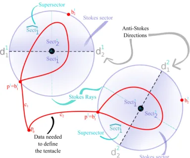
brought together at a single location in the geometry. This question is difficult to answer in the wild Higgs bundle literature, because even having wild ramification at different points requires introducing additional gluing conditions known as tentacles which match the Stokes chambers present near distinct marked points. Additionally, there is always the possibility that additional moduli must be incorporated into the structure of the wild system to properly account for such gluing operations. From the geometric perspective, however, all such moduli spaces are on an equal footing and simply correspond to different parameterizations specified by the singlet moduli of the global F-theory model.
To illustrate, consider anSU(2) 7-brane gauge theory localized on aP1with self-intersection
−2 in an F-theory base. As we have already remarked, 6D anomaly cancellation requires precisely four matter fields in the fundamental representation of SU(2). These matter fields may be localized at distinct points of the curve, or could be collected together at the same point. As we do this, the pole structure, as well as flavor 7-branes of the system will also change. The moduli controlling these deformations are those responsible for moving the locations of marked points. As we establish in Appendix C, such moduli are part of the physical moduli of an F-theory model.
To provide some further examples, in this section we will focus on F-theory compactified on an elliptically fibered Calabi-Yau threefold X → Fn with base a Hirzebruch surface.
Consistency of the model requires −12≤ n ≤12. The minimal Weierstrass model for such geometries is:
y2 =x3+f x+g (5.1)
with:
f(w, u)∼X
i
wif8+n(4−i)(u) (5.2)
g(w, u)∼X
j
wjg12+n(6−j)(u) (5.3)
whereiis bounded by the largest value less than or equal to 8 such that 8 +n(4−I)≥0 and
j is bounded by the largest number less than or equal to 12 with 12 +n(6−J) ≥ 0. Here
w = 0 determines the zero section of the Hirzebruch surface (i.e. the base P1) and u is a local coordinate on the baseP1. By tuning the Weierstrass coefficients, namely by adjusting the values of charged and gauge singlet hypermultiplets, we will show how to interpolate between various types of wild Hitchin systems.
5.1
A Wild Compact
SU
(2)
Model
To illustrate the above points, let us consider an explicit example. We consider an F-theory model with baseFn forna non-negative integer. We will be interested in the case where the
w= 0 locus supports an su(4) gauge symmetry, which is associated with anI4 fiber. Recall that this means f and g must not vanish along w= 0 but the discriminant must vanish to orderw4. Furthermore, we will require that this locus intersects a curve supporting ansu(2) symmetry (i.e. I2 fiber). Producing a product group requires tuning singularities on two loci in the base, w= 0 and w= simultaneously, which is difficult to identify whenf and g
are expanded in w alone. This tuning process was described in [59], where f and g can be systematically expanded in w(w−). Letting σ =w− for brevity:
f =F0+F1wσ+F2w2σ2+. . . (5.4)
g =G0+G1wσ+G1w2σ2+. . . , (5.5)
where Fi =f2i +f2i+1u and Gi = g2i +g2i+1w. For this example, we will set = 1β (note that in the limit 1 →0 this leads to an SU(6) theory).
It is convenient to define thesu(2) locus asσ =w−β1 whereβis a polynomial of degree
r and1 has degree n−rover the P1 base. To leading order the Weierstrass coefficients take the form
f =−α
4β4
48 + 1 18 2α
2β2
1φ−3α2β3ν
w+. . . (5.6)
g = α
6β6
864 + 1 216 3α
4β5ν−2α4β4 1φ
w+. . . (5.7)
with corresponding discriminant locus
∆ =(σ)2 w4
1 5184(α
4
β2)[12βφ3(α2+ 2ν1) +. . .] +O(w) +. . .
(5.8)
where in addition to the functions β and 1, the solution is parameterized by functionsα (of degree 2 +n−r),φ (of degree 4 +r), and ν (of degree 4 +n−r).
The total matter content9 of the theory is determined by the two integers (n and r) and is given in Table 1. It is clear that 1 = 0 counts the bifundamental matter, while α = 0 corresponds to the (6,1). Intersections with the I1 component of the discriminant gives 2n + 16 + 2r (4,1) multiplets and 2n + 16 +r (2,1) multiplets. The locus with β = 0 corresponds to a D5 enhancement which gives r2 (6,2) multiplets. Observe that especially for the SU(4) gauge theory, we have matter fields in different representations. This can
9The singlet moduli counted above are only those contributing on the patch containing w = 0. The
degrees of freedom infi withi≥4 andgj withj ≥6 are unconstrained and omitted from the count above.
In the heterotic dual theory these degrees of freedom are merely the 20 moduli of the heteroticK3 and the
Representation Multiplicity Representation Multiplicity (1,1) 4n−2r+ 22 (4,1) 2n+ 2r+ 16
(6,2) r2 (4,2) n−r
(1,2) 2n+r+ 16 (6,1) n−r+ 2
Table 1: The multiplicity of matter fields (in full hypermultiplets) in the SU(4) × SU(2) theory on base Fn.
also be covered in a local model, and the Hitchin system for such a case has recently been studied for example in reference [60]. It is illuminating to consider the degrees of freedom visible only on theSU(2) component of the discriminant locus in the case that there are no (6,2) anti-symmetric fields. In this case r = 0 and we have n bifundamentals and 2n+ 16 fundamentals ofSU(2). There are 4n+22 total moduli of the system, plus 3n+18 additional
SU(2) singlets not visible from theSU(2) component of the discriminant (i.e. matter in the (4,1) and (6,1) representations). The previously mentioned example of a local −2 curve with SU(2) gauge theory corresponds to the special case where we take n =−2 and r= 0. Note that in this case, we cannot retain the SU(4) enhancement locus. Indeed, otherwise some of the entries in Table 1 would have negative multiplicity.
Let us now turn to the Hitchin system interpretation of this model. Assuming we have tuned the moduli of the Weierstrass model to have an SU(4)×SU(2) gauge theory, we see that we actually have two Hitchin systems which are coupled via the source terms provided by the localized matter. Additionally, we see that generically, different sorts of bifundamen-tal representations will be present. Now, from the perspective of the parent gauge theory described in section 4, we also observe that poles in the Higgs field require background val-ues for a single hypermultiplet. In other words, even if we try to tune the moduli so that different matter fields localize at the same point of a curve, there is no pairing available between different matter field representations. So in this sense, these tunings of different representations cannot change the pole order, but only the location of non-zero entries for each generalized residue.
Assuming that all such localized matter are kept at distinct points, we see that from the perspective of theSU(2) factor, we can engineer only simple poles. Even so, it should still be noted that in this case it is nonetheless possible to achieve a generic T-brane configuration for the SU(2) factor. Conversely, we also see that for the SU(4) factor, the presence of different representations, such as the 6 and 4, and the respective multiplicities allows us to fill out T-branes with simple poles.