Quantitative modelling of the response of earthworms to metals

Cover Page

The handle http://hdl.handle.net/1887/25885 holds various files of this Leiden University

dissertation

Author

: Qiu, Hao

Quantitative modelling of the response of earthworms to metals

Hao Qiu

© 2014 Hao Qiu

Quantitative modelling of the response of earthworms to metals

Ph.D. Thesis Leiden University, The Netherlands ISBN: 978-94-6182-454-7

Cover design: Hao Qiu

Quantitative modelling of the response of earthworms to metals

Proefschrift

ter verkrijging van

de graad van Doctor aan de Universiteit Leiden, op gezag van de Rector Magnificus Prof. mr. C.J.J.M. Stolker,

volgens besluit van het College van Promoties te verdedigen op dinsdag 10 juni 2014

klokke 11:15 uur.

door

Hao Qiu geboren te Jiangsu

Promotiecommissie:

Promotor: Prof. dr. W.J.G.M. Peijnenburg

Co-promotor: Dr. M.G. Vijver

Overige leden: Prof. dr. A. Tukker (Leiden University)

人總是在圖安穩的同時有一顆飛揚的心…

Chapter page

1. General Introduction 9

2. Predicting Cu toxicity to different earthworm species using 27

a multicomponent Freundlich model

3. Modelling Cd and Ni toxicity to earthworms with the free ion approach 47

4. Can commonly measureable traits explain differences in metal 69

accumulation and toxicity in earthworm species?

5. Interactions of Cd and Zn impact their toxicity to the earthworm 87

Aporrectodea caliginosa

6. General Discussion 113

Bibliography 127

Summary 142

Samenvatting 145

Acknowledgements 148

Chapter I

Chapter I

10

1.1 Soil system and metals

Soil is a crucial component of the earth’s ecosystem. As the largest biodiversity reservoir on our planet, soil provides habitat for billions of organisms, including bacteria, fungi, protozoa, nematodes, earthworms, arthropods, plants, et cetera (Baskin, 2005). Soil biodiversity underpins various ecosystem processes and functions which deliver benefits to mankind (ecosystem services) (Blouin et al., 2013). Human activities are increasingly causing degradation and impoverishment of soil and decline in biodiversity which in turn threatens to diminish the capacity of the earth to sustain us. This creates a sense of urgency for us to prevent biodiversity loss, to protect soil functioning and to maintain sustainability of ecosystems. Soil is a dynamic and heterogeneous environment consisting of solid, liquid, and gas phases. The solid phase includes organic material and mineral particles, the liquid phase contains dissolved organic matter and dissolved nutrients, and the gas phase is composed of volatile organic substances and various gases. Soil textures are classified according to the relative proportions of sand (0.05mm - 2mm), silt (0.002mm - 0.05mm) and clay (< 0.002mm) present in a soil (Davis and Bennett, 1927). Various soil constituents show a great capacity to adsorb and retain metals (Van Leeuwen and Hermens, 2007). As a result, soil may act as a sink for the metals released into the environment.

Sources of metals

Metals are naturally occurring components in the environment, with their occurrence primarily in rocks. The release of metals to soil is facilitated by weathering of parent rock and atmospheric deposition (Reeder et al., 2006). Consequently, natural concentrations of metals in soils are strongly correlated to the varied distribution of rock types and vary on a large scale between different geographic regions (Alloway, 1995). Elevated concentrations of metals in the soil environment mainly result from anthropogenic activities such as the extraction, smelting, and processing of bearing ores, the distribution and use of metal-containing products, and the return of concentrated metals through the disposal of processing wastes and the discard of spent products (D’Amore, et al., 2005). These human activities have interfered with the biogeochemical cycles of metals that occur slowly in the natural environment.

Metal behavior

partitioning of metals reflects the differences in chemical behavior and mobility of metals in different soils, to a large extent determining availability of metals to organisms and effects. Metal effects

Concerns about the input of metals to soil are related to their ecotoxicological impact on organisms living in the soil. Next to effects on soil organisms, metal may be transferred via the food chain, resulting in health effects on animals and humans. Several metals (e.g., Cu, Ni, and Zn) are essential for living organisms because they play an important role in various biochemical and physiological processes, while some (e.g., Cd, Pb, and Hg) are highly toxic and have no known physiological function (nonessential) (Peijnenburg et al., 2007). There is an optimal level of essential metals for maximum benefit. Below this level symptoms of metal deficiency may occur whereas above this level the metal may become less beneficial and eventually toxic with increasing levels of availability (Hopkin, 1989). Toxic effects of metals on soil invertebrates (e.g., earthworms, enchytraeids, and nematodes) and microorganisms are reduced species diversity, abundance, and biomass (Bengtsson and Tranvik, 1989; Santorufo et al., 2012) and changes in microbial processes (e.g., glucose induced respiration and potential nitrification rate) (Oorts et al., 2006; Vig et al., 2003). Effects of metals on vascular plants can be reflected in the form of toxicity symptoms (reduced development and growth of shoots and roots) (Le et al., 2012), physiological symptoms (decreased nutrient contents in leaf tissues, elevated concentrations of total sugar and starch) (Prasad 1995), and biochemical symptoms (decreased enzymatic activity) (Das et al. 1997; De Vries et al., 2007). These effects could have serious consequences for soil biodiversity, and in turn soil functioning and ecosystem sustainability. Therefore, an understanding of the actual risks posed by metals in soil is needed.

Metal risk assessment

Ecological risk assessment for metals in soil is routinely conducted based on laboratory data from standardized ecotoxicity tests using selected terrestrial species (e.g., earthworms, Enchytraeids and Collembola) (Løkke and Van Gestel, 1998). These ecotoxicity tests focus on establishing quantitative concentration-effect relationships so that toxicity thresholds and therefore risk limits can be derived. This information is required in the modern regulatory system of the European Union - REACH (Registration, Evaluation and Authorization of Chemicals). REACH makes industry responsible for assessing and managing the risks posed by metals and other chemicals. Recently, there are also new moves toward establishing a Chinese REACH system: two guidelines concerning risk assessment under the order No.7 of the Ministry of Environmental Protection of China are pending (MEP, 2011). The original

Guideline for the Hazard Evaluation of New Chemical Substances (HJ/T 154-2004) is revised

into two separate documents, the Guideline for Risk Assessment of Chemicals and the

Guideline for Hazard Identification of New Chemical Substances. The (draft) Guideline for

Chapter I

12

To date, soil quality criteria and risk assessment of metals are still predominantly based on total concentrations (Janssen et al., 2003). However, efforts to relate the total concentration of a metal to toxic effects have proven difficult (Reeder et al., 2006). Metal toxicity, even to the same organisms, can vary largely in different soils because of the impact of soil properties and metal bioavailability, which affects the relevant exposure concentration for organisms (Rooney et al., 2006; Criel et al., 2008; Santorufo et al., 2012). Improving the accuracy of the risk assessment and decision making requires an explicit consideration of bioavailability and other ecological knowledge.

1.2 Bioavailability

The concept ofbioavailability was introduced to consider the fraction of a contaminant that will actually have an effect on organisms (Patrick et al., 1977; Mayer, 2002). However, bioavailability cannot be directly related to toxic effects as the latter follow from the amount of metals that react with the target sites of cells (Peijnenburg et al., 2007). As such, bioavailability can be considered a three-step approach, in which the available metal causes exposure (environmental availability), exposure leads to dynamic or passive uptake (environmental bioavailability), and subsequent effects result from reaction with a biological target (toxicological bioavailability) (Figure 1.1) (Dickson et al., 1994; Landrum et al., 1994; Peijnenburg et al., 1997).

the metal across the membrane of orgamism (environmental bioavailability). The amount of accumlated metal that reacts with the target sites determines the subsequent effects (toxicoligical bioavailability).

Metals exist in different solid-phase and solution-phase forms that can vary greatly in terms of their bioavailability. Although the majority of metals are in the soil solid phase, metals in the solution phase pose the largest risks for soil dwelling organisms (Groenenberg, 2010). Metals in the soil solution are far more mobile and available than those in the solid phase (De Vries et al., 2005). Uptake by soil organisms via soil solution is supposed to be the most relevant pathway for metal exposure (Van Gestel and Koolhaas, 2004; Vijver et al., 2003). When a metal is supplied from the solid phase, it must first be transferred to solution before it can be taken up. Furthermore, not all dissolved metal species in the solution phase are readily available for uptake by organisms (Zhang et al., 2004). Therefore, the metal concentration and speciation in the soil solution are the major aspects that govern bioavailability. Extensive studies have reported that soil properties which control metal partitioning and speciation, such as pH, organic matter content, clay content, cation exchange capacity and the concentration of Fe- and Al-oxyhydroxides, have a significant influence on bioavailability (Janssen et al., 1997; Peijnenburg et al., 1999; Oorts et al., 2006; Smolders et al., 2009).

Besides physiochemical properties of the soil, biological processes may also play an important role in controlling bioavailability. For example, earthworms appear to affect metal bioavailability through stimulating soil microbial population, altering pH and DOC of the soil solution (Sizmur and Hodson, 2009). Plants can change metal bioavailability through root activities and related rhizosphere processes (rhizosphere acidification or root proliferation and secretion of organic acids). Mench and Martin (1991) reported that soil Cu, Cd, Ni, Zn, Fe, and Mn were dissolved by root exudates of corn.

Chapter I

14

chemical insights in metal speciation with biological insights regarding effects, have been developed. These models will be introduced below.

1.3 Effect modelling

Already for a long time researchers attempt to understand the exact mechanisms that induce differences in bioavailability and subsequent toxicity across water and soils. It has been recognized that metal bioavailability and toxicity are to a large extent controlled by the free ion activity in (soil) solution (Morel, 1983; Campbell, 1995; Batley et al., 2004; Van Gestel and Koolhaas, 2004). Based on these assumptions, mechanistically underpinned models such as the free ion activity model (Morel, 1983), the biotic ligand model (Di Toro et al., 2001) and the electrostatic model (Wang et al., 2008) were developed. Given the global desire of minimizing animal testing and reducing costs of regulatory testing of chemicals (Höfer et al., 2004), these modelling approaches are favorable for conducting ecological risk assessment of metals.

Free ion activity model

The bioavailability models for predicting metal toxicity were initially developed for the aquatic environment. In 1983, François Morel published a book “Principles of Aquatic Chemistry”, which led to the development of the conceptual free ion activity model (Morel, 1983). The model describes how variations in the effect levels of metals can be related to their aqueous speciation and interactions with the organism (Morel, 1983; Paquin et al., 2002). It is assumed that among the various metal species, only the free metal ion can bind to the active sites (carrier, channel or toxic action sites) of the cell surface membrane, and subsequently be transported across the membrane to induce toxic effects (Morel, 1983; Campbell, 1995; Brown and Markich, 2000). Interactions between a metal ion and an organism generally involve three steps: (1) diffusion of the metal ion in the bulk solution to the surface of the cell membrane; (2) sorption or surface complexation of the metal ion at the active sites of the cell membrane; (3) uptake or transport of the metal ion across the cell membrane of the organism (Campbell, 1995). The key assumption which underpins the free ion activity model is that there is a rapid equilibrium between metal ions in the solution and those at the cell membrane (as follows):

{Mz+_{} + {-R}

cell} ↔ {M-Rcell} (1-1)

that is,

{M-Rcell} = k1 {Mz+} {-Rcell} (1-2)

where {Mz+_{} is the free metal ion activity, {-R}

proposed and developed to consider both chemical speciation and ion competition in estimating metal toxicity (Di Toro et al., 2001; Paquin et al., 2000; Santore et al., 2002). Biotic ligand model in the aquatic environment

The biotic ligand model (BLM) is a theoretical framework in which toxicity is related to the binding of metal ions to the sites of toxic action on an aquatic organism. For modelling purposes, the sites of toxic action are treated as a biotic ligand, that is, the biological counterpart of chemical ligand to which metals can bind. Toxic effects occur when the concentration of metal-biotic ligand complex reaches a certain critical level (Di Toro et al., 2001). The model also considers that other dissolved constituents that are present in the aquatic environment can influence the extent of metal binding to the biotic ligand. These constituents may either reduce the concentration of metal-biotic ligand complexes by competing with the metal for binding at the biotic ligand (e.g., Ca2+_{, Mg}2+_{, Na}+ _{and K}+_{) or by} the formation of dissolved complexes with the metal (e.g., dissolved organic carbon, inorganic ligands) (Figure 1.2) which reduce the free metal ion activity. The principal feature in the BLM is the competition of the free metal ion with other cations for binding at the biotic ligand. This feature distinguishes the BLM from earlier concepts that considered only the free metal ion as the toxic species. The metal-organism interaction part of the biotic ligand model is based on the free ion activity model.

Figure 1.2 Schematic diagram of the framework of Biotic Ligand Model. For further information see the text and Di Toro et al. (2001).

Chapter I

16

physiological processes involved in ion-regulation between the organism and the external environment. The most important adverse effects of metals on aquatic organisms have been demonstrated to involve the disturbance of the organisms’ ability to regulate their internal ion balance. Three principal categories of physiological mechanisms of toxicity are distinguished: monovalent metals affecting Na+ _{transport, divalent metals affecting Ca}2+ _{metabolism, and} metals that affect the organism centrally after passing the gill. Paquin et al. (2002) refer to various experimental studies demonstrating that metal accumulation at the site of toxic action is truly a function of metal complexation and competitive interactions, as conceptualized in the earlier models such as the gill surface interaction model (Pagenkopf, 1983) and the free ion activity model (Morel, 1983).

According to the assumption of the BLM, metal ions (Mz+_{) and other cations (H}+_{, K}+_, Ca2+_{, Na}+_{, and Mg}2+_{) can bind to the theoretical biotic ligand (BL) sites (De Schamphelaere} and Janssen, 2002). The interaction between cations and BL is treated as a surface complexation reaction. At equilibrium, for example, the stability constant for Mz+ _{binding to} biotic ligands KMBL (L/mol) can be expressed as a function of the concentrations of cation-biotic ligand complexes [MBL] (mol/L) and unoccupied cation-biotic ligand sites [BL] (mol/L):

_{{ }} (1-3)

where {Mz+_{} is the free metal ion activity (mol/L).}

Metal toxicity is assumed to be proportional to the fraction (f) of the total biotic ligand sites [BL]T occupied by the toxic metal. The f value depends on the binding affinity of M2+ to the BL and the presence and binding affinity of the competing cations (De Schamphelaere and Janssen, 2002):

{ }

{ } ∑ { } (1-4)

where {XZ+_{} is the activity of major cations (Ca}2+_{, Mg}2+_{, K}+_{, and Na}+_{) in the solution, K} XBL is the binding constant of cations XZ+ _{bindingto the BL.}

The biological response is related to f using the logistic dose-response relationship:

(

)

(1-5)

where R is the survival rate, Ro is the control survival rate, f50 is the fraction of the total BL sites occupied by M2+ _{at which the survival rate is reduced by 50%, β is the slope parameter.}

The value of f at the 50% effect level is assumed to be constant according to the BLM theory. Equation 2 then can be rewritten as:

{ _}

( ) { ∑ (

_{)} (1-6)}

where EC50{Mz+_{} is the free metal ion activity inducing 50% effect. The BLM parameters}

(De Schamphelaere and Janssen, 2002;Deleebeeck et al., 2009). The validity of the BLM can be established only if the critical concentration is the same over the entire range of environmental conditions that have been tested. A speciation model (e.g., WHAM) is needed for the necessary calculations. A major strength of the BLM is that it provides a mechanistic and operational framework for interpreting the effects of exposure water chemistry on metal bioavailability and toxicity. Many aquatic BLMs have been successfully developed and applied to predict metal toxicity to fish, algae, and water fleas in different exposure conditions (Alsop et al., 2000; De Schamphelaere and Janssen, 2004; Heijerick et al., 2002; Santore et al., 2002). The toxic effects estimated by these BLMs are generally within a factor of two of the observed toxic effects. Some exceptions are also reported especially in alkaline exposure conditions (De Schamphelaere and Janssen, 2002; Li et al., 2009a, Wang et al., 2009). Metal speciation changes substantially over the alkaline pH range and species other than the metal ion dominate in the solution (Wang et al., 2012). It has been suggested that the effect of pH on metal toxicity at a relatively high pH (>8) is a speciation effect rather than significant competition effects between protons and metal ions (De Schamphelaere and Janssen, 2002; Markich et al., 2003; Wang et al., 2010). In addition to free metal ions (e.g., Cu2+_{), other metal forms (e.g., CuOH}+ _{and CuHCO}

3+) may also contribute to toxicity at pH-values exceeding 8. There is also the possibility of physiologically initiated modification of the structure of the membranes at high pH levels (Lavoie et al., 2012). Therefore, the applicability of BLM in high-pH media needs to be investigated further.

Biotic ligand model in the terrestrial environment

According to the BLM theory, toxicity occurs as a consequence of free metal ions reacting with the biotic ligand at the interface of solution and organism (Di Toro et al., 2001). It is assumed that the toxicity principles for fish and other aquatic species are also applicable to terrestrial species such as earthworms and plants. In case of these specific terrestrial organisms, the sites of toxic action are in direct contact with the external (soil) solution. This is an evolutionary phenomenon as general binding sites such as sodium and calcium transporters are inherent to every living cell (Niyogi and Wood, 2004). By considering the biotic ligand as a more general binding site, the principles underlying aquatic BLMs are likely to be valid also for terrestrial species. Attempts have been made to develop BLMs for soil invertebrates (earthworms and enchytraeids) (Steenbergen et al., 2005; Li et al., 2008; Lock et al., 2006) and plants (Lock et al., 2007; Li et al., 2009a) in solution or in solution-sand systems. These studies show that the application of the BLM to terrestrial organisms is theoretically and empirically feasible. One of the key limitations of these studies lies in the difficulty to relate the observed results to real world conditions. Increasing our understanding of the mechanisms behind metal uptake and toxicity to soil species is valuable, but the mechanistic information needs to be relevant with regard to the actual exposure of organisms in natural soils, for the terrestrial BLMs to be truly meaningful. The geochemistry of the hydroponic conditions bears little resemblance to that of real world soils, and identifying the challenges that are anticipated in soil validation of these systems would be appropriate.

Chapter I

18

the solution by sorption to reactive solid phases, such as the soil organic matter (SOM), and the mineral (hydr)oxides of Fe, Al, and Mn, and clay. Competitive sorption of cations, protons, etc., to these solid phases also affects the distribution of the metal between the soil solid phase and solution. Free metal ions (M2+_{) can form complexes with dissolved organic} and inorganic ligands. A speciation model is needed to determine the metal speciation in solution, but such a model needs to account also for the partitioning of the metal between the soil solution and the soil solid phase. In addition to these soil geochemical processes that control metal speciation, the terrestrial BLM includes a toxicity model similar to that of the aquatic BLM.

Figure 1.3 Schematic overview of the interactions considered in the terrestrial biotic ligand model (Thakali et al., 2006a).

physicochemical properties of soil (Lofts et al., 2004; Wang et al., 2011a). For example, the amount of protons and major cations released to the soil porewater covaries with the amount of metal salt added in soil (Wang et al., 2011a). Parameterization of the BLM, therefore, faces a variety of challenges and uncertainties. Despite these difficulties, Thakali et al. (2006a, b) developed and applied the BLMs in acidic soils for describing Cu and Ni toxicity to plants (barley, tomato), soil invertebrates (earthworm, springtail) and microbial processes (nitrification potential, respiration). Free metal ions in the soil solution were assumed to be the dominant toxic species while cation competition was supposed to modify toxicity. Interactions between the metal and the soil solid phase, and between the metal and the solution phase were taken into account when calculating metal speciation in soil solution. In applying the BLM to the toxicity data, Thakali et al. found that it is unavoidable to empirically fix some of the BLM parameters (f50 and even one of the binding constants of the protective cations). Therefore, the estimated binding constants should not be regarded as conventional binding constants but rather as parameters that summarize the processes underlying the observed relation between organism responses and competing cations. Since the development of terrestrial BLMs for metals like Cu, Ni, and Cd is not readily feasible, it would be highly desirable to develop alternative methods, which facilitate the application of the BLM theory in soil, to assess metal toxicity to terrestrial organisms.

1.4 Mixture toxicity

In the real world, exposure to metal mixtures is a rule rather than an exception (Kortenkamp et al., 2009). However, current regulatory approaches focus almost exclusively on single metals and rarely require assessment of mixtures, which may have little real environmental relevance (Backhaus and Faust, 2012). The development of simple and efficient approaches for modelling mixture toxicity is necessary in the sense of meeting future regulatory demands and ensuring adequate risk assessment.

The foundations for mixture toxicity modelling have been laid by pharmacologists since 1920s (Loewe and Muischnek, 1926; Bliss, 1939). Conceptual models (see below) were developed by simply adding doses and responses to predict mixture effects based on the assumption that mixture components do not impact each other’s toxicological action. However, the interactions of mixture components that may lead to decreased or increased bioavailability and toxicity were ignored. To date, our understanding of mixture toxicity is still based on those concepts, with addition as the basis for most models (Vijver et al., 2010). Only limited progress has been made to incorporate the interactions of mixture components in predicting mixture toxicity.

Conceptual models (Non-interaction)

Chapter I

20

The CA concept was developed by Loewe and Muischnek (1926) to describe mixtures where the components have the same or a similar mode of toxic action (i.e., act on the same biological pathway and strictly the same molecular target):

∑ (1-7)

where n is the number of mixture components, ci is the concentration of component i in the mixtures causing xi% effect, ECxi is the effective concentration of component i causing xi% effect when applied singly. The term is also defined as Toxic Unit (TU) which scales the relative toxicity of each component (Sprague, 1970). TUmix is therefore a dimensionless quantity that equals the sum of the TUs of the individual components in the mixture. When the EC50 of the mixture equals 1 TUmix, no interactions occur and CA holds. Values of TUmix that are statistically significant below 1 indicate synergism, while values significantly exceeding 1 describe antagonism. CA deals with the issue that the relative toxicity of the metals that are present in the mixtures is the same as the relative toxicity of the metals present individually.

The concept of IA was first proposed by Bliss (1939) to describe mixtures where the components have different modes of action (i.e., act on different physiological systems):

( ) ∏ ( ) (1-8)

where E(cmix) is the predicted effect (scaled in the range of 0-1) of mixtures, ci is the concentration of component i, E(ci) is the effect of component i present singly at a concentration ci. IA addresses the question whether the probability of response to one metal may be independent from the probability of response to another metal. In this model, the relative toxicity potency of metals is ignored, and the mixture effect is predicted from the joint probability of statistically independent events (Peijnenburg and Vijver, 2007).

With regard to the choice for a conceptual model, the basic idea is to use CA if the components are expected to act similarly and to use IA if the components are expected to act dissimilar (Junghans et al., 2006). However, identifying the modes of action for different chemicals is not always possible. In those cases, CA is suggested to be the more conservative choice in a risk assessment context as it estimates a higher response than IA and therefore represents the worst-case scenario for mixture exposure (Lock and Janssen, 2002; Backhaus and Faust, 2012).

Deviations from conceptual models (Interaction)

(1) Non-interaction: the observed mixture effect is adequately explained by either CA or IA.

(2) Absolute synergism or antagonism: the observed effect of all combinations of a

mixture is significantly more severe (synergism) or less severe (antagonism) than the mixture effect predicted by either CA or IA.

(3) Dose ratio dependent deviation: the deviation from the CA- or IA-predicted mixture

effect depends on the relative proportion of mixture components. For example, in binary mixtures, antagonism can be observed when component A dominates toxicity, whereas synergism can be observed when component B dominates toxicity.

(4) Dose level dependent deviation: the deviation from the CA- or IA-predicted mixture

effect depends on the overall mixture concentrations. For example, antagonism can be observed at low dose levels while synergism is observed at high dose levels.

In soil, mixture toxicity is complex to study because metals may interact at various levels (Calamari and Alabaster, 1980): (1) the exposure level, (2) the uptake level, (3) the target level, and (4) the internal pathway of detoxification. The first level deals with physicochemical interactions in the soil matrix, influencing sorption (partitioning of metals between soil solid phase and soil solution) and thereby the bioavailable fraction of metals. The second level involves physiological interactions during the uptake processes by the organisms, which affect toxicokinetics and subsequently the quantity available at the sites of action. The third and fourth levels describe interactions of metals at the receptors and target sites, at the intoxication processes, which affect toxicodynamics and hence the joint effect (Weltje, 1998; Conder and Lanno, 2000). Insight into these interaction levels and their relative importance is of great value for toxicity assessment of metal mixtures. This information will help to generalize study results between metal mixtures, as well as between different soil types and organisms.

Incorporation of bioavailability into mixture toxicity modelling

Another challenge in predicting mixture effects results from differences in the bioavailability and approaches used to define the bioavailable fraction among toxicological studies and subsequent ambiguity in interpreting mixture toxicity data (Peijnenburg and Vijver, 2007). For example, different conclusions (antagonistic, more antagonistic, additive) on mixture interactions were drawn when using different expressions of exposure (total soil concentration, CaCl2-extractable concentration, internal concentration) (Bongers, 2007). The 0.01 M CaCl2-extractable metal concentration or porewater concentration is often considered to be a suited estimate of the available metal pool for soil organisms (Peijnenburg et al., 2007). Therefore, all these expressions of exposure are considered in our research. Understanding the chemical interactions in soil could help in the interpretation of different outcomes of studies working with soils of different types.

Chapter I

22

hence, to predict metal toxicity using the BLM in a CA model. Alternatively, if competitive binding does not occur, then the BLM may provide more reliable estimates of bioavailability of individual metals, which can then be incorporated into a more accurate IA model.

1.5 Species-specific responses

Metal accumulation and effects are not only driven by abiotic factors like chemical speciation and cation competition. Organisms themselves have developed effective strategies to cope with metal exposure. They have the ability to excrete or eliminate the metal to control metal accumulation and maintain homeostasis over a certain level of exposure (Chapman et al., 1996; Wood, 2001). They are also able to minimize toxic effects of reactive forms of metals in their body by sequestration, detoxification, and storage (Vijver et al, 2004). These physiological processes of organisms have not been accounted for when assessing the risks posed by metals in the environment. Studies have shown that metal accumulation and excretion rates are species dependent. Rapid zinc uptake and elimination was found in

Eisenia fetida (Spurgeon and Hopkin, 1999), while slow uptake was found in Lumbricus

rubellus (Mariño and Morgan, 1999). Janssen et al. (1991) studied the accumulation and

elimination kinetics of cadmium in four arthropod species and observed large differences between species, which could mainly be attributed to species-specific differences in accumulation strategies. Variations in sensitivity to a given metal have been reported widely between different species. For example, Spurgeon et al. (2000) found that the earthworms L.

rubellus and Aporrectodea caliginosa were more sensitive to Zn than L. terrestris and E.

fetida. Langdon et al. (2005) reported that the sensitivity of three earthworm species to Pb

followed the decreasing order: L. rubellus > A. caliginosa > E. fetida. This can be a result of species-specific differences in physiological characteristics that determine detoxification and elimination strategies (Dallinger, 1993). In addition, the activity of calcium glands in earthworms may partially account for the differences in sensitivity as calcium is involved in the sequestration and elimination of many metals. It has been suggested that the more tolerant species E. fetida and L. terrestris have a higher calcium gland secretion activity than the relatively sensitive species (Morgan and Morgan, 1991; Spurgeon and Hopkin, 1996). Other species characteristics (e.g., time to maturity, habitat, food choice, immune-competent cells, etc.) may also affect metal accumulation and toxicity (Edwards and Bohlen, 1996; Plytycz et al., 2011a). More research efforts are needed on this aspect to establish solid links between species-specific responses and the relevant traits (i.e., specific characteristics of species) and processes. The exploration of such an approach, that is a traits-based approach (Baird et al, 2008; Rubach et al, 2012), might assist in explaining why one species is more sensitive to metals than another species and allows for extrapolating the results of metal accumulation and toxicity over species.

1.6 Earthworms

formation (Peijnenburg and Vijver, 2009). They are also valued for their contribution to ecosystem services (i.e., provisioning, regulating, supporting and cultural services) through their action on soil processes (Blouin et al., 2013). Earthworms are commonly considered as soil ecosystem engineers because they benefit the soil ecosystem in a number of ways: mixing soil layers, recycling organic matter, increasing nutrient availability, improving soil aeration, and enhancing microbial activity, et cetera (Edwards and Arancon, 2004; Blouin et al., 2013). As earthworms play a unique role in sustaining the essential functions of soil, detrimental effects of metals on earthworms may indirectly harm soil health and subsequently the whole ecosystem.

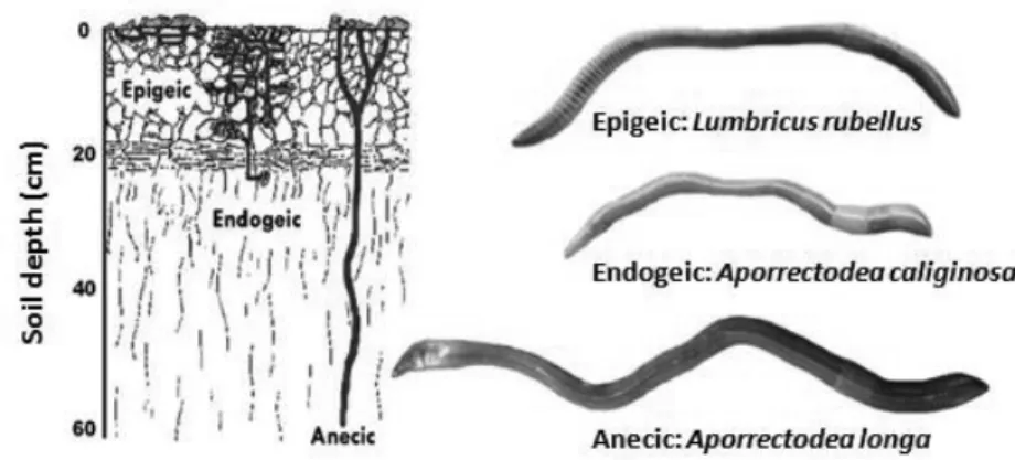
Different species of earthworm have different habitats, behaviors, and life histories and occupy different niches within the soil ecosystem (Domınguez, 2004). Earthworm species are generally divided into three different functional groups based on their ecological strategies (Bouché, 1977): epigeic, endogeics, and anecic (Figure 1.4). Epigeic species live in the soil surface layer and feed on litter and organic rich materials. Endogeic species live in the mineral layer of the soil and feed on soil and associated organic matter. Anecic species live in deep vertical burrows but feed on litter at the soil surface (Domınguez, 2004). The Figure 1.4 illustrates where the earthworms live (their habitats), indicating that these earthworm species occupy different ecological niches.

Figure 1.4 Earthworm functional groups and representative species of each group. Figure adapted from Fraser and Boag (1998) (slightly modified).

Chapter I

24

Determination of Effects on Reproduction of Eisenia fetida/Eisenia andrei, ISO 11268-2: 2012” (ISO, 2012). These guidelines are designed to estimate critical effect levels from concentration-response relationships for survival and/or reproduction of mature earthworms.

Earthworms are ideal organisms for assessing the toxicity of metals to soil-dwelling species, because they are in intimate contact with the soil porewater and the soil solid phase. Thus, they are exposed in a manner representative of many soil species, including bacteria, plants, and other soft-bodied invertebrates. Earthworms have a water-permeable surface epithelium. Although direct uptake via the gut wall (food) cannot be completely ruled out, many findings have suggested that metal uptake by earthworm takes place predominantly via the porewater or via an uptake route that is related to porewater uptake (i.e., the porewater hypothesis) (Saxe et al, 2001; Vijver et al., 2003; Jager et al., 2003; Van Gestel and Koolhaas, 2004). Vijver et al (2003) investigated a method (oral sealing using glue) to distinguish different uptake routes of metals in earthworms and found that the dermal route is the main uptake route. Janssen et al (1997) found that the same soil properties affecting metal partitioning between the soil solid phase and soil porewater were also the dominant soil properties affecting metal accumulation in earthworms. In our study, the porewater hypothesis was adopted. Metal in soil porewater is assumed to dominate toxic effects, which connects the soil solid phase and the organism.

Four earthworm species (Eisenia fetida, Lumbricus rubellus, Aporrectodea caliginosa

and Aporrectodea longa) were used in the present study. The epigeic E. fetida is an

artificially cultured species that inhabits only organic matter-rich locations. They are rarely found in natural soil. L. rubellus,A. caliginosa and A. longa are the representatives of epigeic, endogeic, and anecic earthworm species living in natural soil, respectively (Figure 1.4) (Spurgeon et al., 2000). The differences in ecological strategies and physiological characteristics between species may strongly affect effective exposure and toxicity (Morgen and Morgen, 1999). Taxonomy is not an inherently informative indicator for prospective risk assessment of metals, as two species of the same genus may show large differences in sensitivity. However, the phylogenetically related aggregations of certain species traits may provide a clue for species-specific accumulation and toxicity (Rubach et al. 2010). It has been suggested that uptake processes are physiologically driven and affected by species specific parameters (traits) such as morphology, soil habitat, feeding strategy and preferences, and life history (Peijnenburg et al., 2012). Species may possess different trait combinations to cope with a particular disturbance (De Lange et al. 2013). Incorporating traits-based approaches in metal toxicity assessment is supposed to give more explanatory power and allows for extrapolation of results of metal accumulation and toxicity between different earthworm species.

1.7 This thesis Objective

understanding bioavailability and developing appropriate bioavailability models for soil organisms. Therefore, the specific goals of this thesis were:

1. To develop bioavailability models to facilitate the application of BLM theory in soils;

2. To model mixture toxicity by taking into account the interactions of mixture components at different toxicological levels;

3. To extrapolate the study results to other studies reported in the literature.

To accomplish these goals, the following research questions were addressed:

[1] Which cations (H+_{, Ca}2+_{, Mg}2+_{, K}+ _{and Na}+_{) exert significant effects on metal} toxicity and how could these toxicity-modifying factors be incorporated into terrestrial toxicity models developed on the basis of the BLM theory? (Chapters II and III)

[2] Are the toxicity-modifying factors the same for different earthworm species

(Lumbricus rubellus, Aporrectodea longa, and Eisenia fetida) and for different

metals (Cu, Cd, and Ni)? (Chapters II and III)

[3] Are metal (Cu, Cd, Ni, and Zn) accumulation pattern and sensitivity of earthworms species-specific? Can species-specific traits of earthworms provide a clue for predicting metal accumulation and toxicity? (Chapter IV)

[4] Where do the interactions of mixture components (Cd and Zn) possibly occur and

how do they impact the observed toxicity? (Chapter V)

Biotic ligand models are increasingly being developed and applied to relate toxic effects of metals on aquatic organisms to activities of the free metal ion and competing ions. We have adopted the recent hypothesis that this modelling theory is also applicable to organisms in the soil environment. It is expected that free metal ions in soil porewater are mainly responsible for toxicity while the base cations can mitigate toxicity through competition for binding to the biotic ligand sites. Trait-based approaches are used to assist in explaining differences in metal accumulation and toxicity between earthworm species living in different habitats, with ultimately the idea to enable cross-species extrapolation of accumulation and toxicity data. Since mixture exposure represents realistic field scenarios and since mixture interactions at different toxicological levels may impact the actual risks, attempts are made to determine where mixture interactions could occur and to quantify the toxicity deviations from simple concentration addition, ultimately ensuring adequate risk assessment.

Thesis outline

This Chapter provides an overview of the basic principles of speciation, bioavailability

and effect modelling of heavy metals in the terrestrial environment, particularly with regard to the development of biotic ligand models and mixture toxicity models. The main issues were highlighted and ways to tackle the associated problems were discussed.

The research questions are answered in the following chapters:

Chapter II: A Freundlich-type model, rather than the biotic ligand model, was proposed

Chapter I

26

complies with the basic assumptions of the biotic ligand model but requires fewer parameters than the biotic ligand model, thus facilitating the application of biotic ligand model principles in soil exposure systems. The possibility of extrapolating the study results to other studies reported in literature was also explored.

Chapter III: When applying the BLM to the soil system, parameterization of the BLM

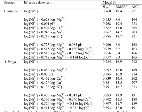
faces a variety of challenges and uncertainties. Based on empirical studies and BLM theory, here we proposed an alternative method, the free ion approach, to predicting Cd and Ni toxicity to earthworms (L. rubellus and A. longa). Previously, the applicability of the free ion approach for describing Cu toxicity has been proven. However, the toxicity-modifying factors (H+_{, Ca}2+_{, Mg}2+_{, Na}+_{, and K}+_{) are shown to be different for other metals. Results} obtained from our study strongly suggest that metal toxicity to earthworms needs to be evaluated on a metal-specific basis.

Chapter IV: It is often stated that there is not enough ecology in ecotoxicology and that this lack can have unfortunate consequences for environmental risk assessment. Here we examined the differences in metals (Cu, Cd, Ni, and Zn) accumulation and toxicity in three earthworm species (L. rubellus, A. longa and E. fetida), with a special focus on the impact of earthworm traits. In this study, the ecophysiological differences between earthworms were identified and used to assist in explaining metal accumulation patterns and sensitivity. These species-specific traits of earthworms are expected to provide a clue for extrapolation across species.

Chapter V: The toxic unit method was used to quantify the mixture (Cd and Zn) toxicity in one earthworm species(A. caliginosa). Deviations caused by mixture interactions were assessed using the MIXTOX model. Interactions associated with different expressions of exposure (total, CaCl2-extractable, and porewater concentrations) were compared. In soil, mixture toxicity is complex to study because interactions of metals can occur at various levels. By separating the interactions at the exposure level from the uptake level and the target level, it was determined where the interactions possibly occur and their influence on the toxicity pattern of binary metal mixtures was subsequently assessed.

Chapter II

Predicting Copper Toxicity To Different Earthworm Species Using A Multicomponent Freundlich Model

Hao Qiu, Martina G. Vijver, Erkai He, Willie J.G.M. Peijnenburg

Chapter II

28

Abstract

This study aimed to develop bioavailability models for predicting Cu toxicity to earthworms (Lumbricus rubellus, Aporrectodea longa, and Eisenia fetida) in a range of soils of varying properties. A multicomponent Freundlich model, complying with the basic assumption of the biotic ligands model, was used to relate Cu toxicity to the free Cu2+ _activity and possible protective cations in soil porewater. Median lethal concentrations (LC50s) of Cu based on the total Cu concentration varied in each species from soil to soil, reaching differences of approximately a factor 9 in L. rubellus, 49 in A. longa and 45 in E. fetida. The relative sensitivity of the earthworms to Cu in different soils followed the same order: L.

rubellus > A. longa > E. fetida. Only pH not other cations (K+_{, Ca}2+_{, Na}+_{, and Mg}2+_{) were}

found to exert significant protective effects against Cu toxicity to earthworms. The Freundlich-type model in which the protective effects of pH were included, explained 84%, 94%, and 96% of variations in LC50s of Cu (expressed as free ion activity) for L. rubellus, A.

longa, and E. fetida, respectively. Predicted LC50s never differed by a factor of more than 2

2.1 Introduction

Soil contamination with metals poses a serious threat to soil functions and sustainability of ecosystems (De Boer et al., 2011). A large amount of Cu discharge comes with the widespread use of this metal, for example, in mining industry as a floatation reagent and in agriculture as a fungicide or fertilizer (Gimeno-García et al., 1996). This strengthens the need to develop appropriate quality criteria and predictive models to evaluate to what extent and what magnitude Cu poses risks to soil organisms.

Numerous studies have shown that uptake and effects of metal depend on species, soil type and metal bioavailability (Nahmani et al., 2007; Peijnenburg et al., 2007; Van Gestel et al., 2004). To induce potential effects, metal should be bioavailable for being taken up by soil organisms (Peijnenburg et al., 2007). The porewater hypothesis proposes that exposure takes place via the porewater or that uptake of metal is mediated by a porewater related route (Van Gestel and Koolhaas, 2004; Vijver et al., 2003). The free metal ion in soil porewater is supposed to be the potential toxic species that is actually taken up by soil organisms (Morel, 1983; Peijnenburg et al., 1999). This forms the theoretical basis of using the free metal ion to predict uptake and toxicity and leads to the free ion activity model (Morel, 1983). The development of the biotic ligand model (BLM) is an extension of the free ion activity model (Campbell, 1995; De Schamphelaere and Janssen, 2002). It considers metal speciation and competition with other cations (e.g., H+_{, Na}+_{, K}+_{, Ca}2+_{, Mg}2+_{). Toxicity is assumed to be} proportional to the fraction of the total biotic ligand sites (transport sites or physiologically active sites) occupied by the toxic metal (De Schamphelaere and Janssen, 2002; Niyogi and Wood, 2004). Initially BLMs were proposed as a tool to quantitatively predict metal toxicity for aquatic organisms. However, the principles underlying aquatic BLMs are likely to be valid also for terrestrial species (Plette et al., 1999), especially when exposure is predominantly via the dermal route and soil organisms (such as earthworms) are in close contact with the soil porewater (Steenbergen et al., 2005; Vijver et al., 2003).

Van Gestel and Koolhaas (2004) studied the toxicity of Cd to the springtail Folsomia

candida and found that besides the free Cd ion activity, pH in soil porewater or in water

Chapter II

30

Some cases suggested the usefulness of the BLM to predict metal toxicity in soil, while others showed exceptions (Lock et al., 2006; Steenbergen et al., 2005; Thakali et al., 2006a; 2006b). This raises the question of whether the BLM concept is too simplified for complex soil processes.

When developing BLMs for terrestrial organisms, solution system, instead of the real soil, is often used in order to simplify the complex soil processes (Lock et al., 2006; Steenbergen et al., 2005). There may be two problems hindering the development of BLMs directly from soil system and the interpretation of data. Unlike the solution system, it is difficult to univariately modify the parameters that affect metal toxicity in soil. Another difficulty is that the intercorrelation among parameters in soil culture, for example, the amount of H+_{, Ca}2+_{, and Mg}2+ _{released to the soil porewater covaried with the amount of} metal added in soil (Wang et al., 2011a). Even so, the soil exposure system was chosen in the present study considering the environmental reality. A multicomponent Freundlich model (Plette et al., 1999), rather than the BLM, was proposed to link Cu toxicity in different species of earthworms to free Cu2+ _{and possible protective cations in soil porewater. This} model complies with the basic assumptions of BLM but requires fewer parameters than the BLM (Mertens et al., 2007; Ore et al., 2010), facilitating the application of BLM principles in soil exposure system.

The main objectives of the present study were to examine whether the multicomponent Freundlich model, which complies with the BLM concept and incorporates cations competition, can effectively predict Cu toxicity across different earthworm species

(Lumbricus rubellus, Aporrectodea longa, and Eisenia fetida), and to explore the possibility

of extrapolating the study results to other studies reported in literature.

2.2 Materials and methods Soil spiking

Soils of varying properties were collected from six different agricultural sites (Valkenswaard, Boxtel, Woerden, Drimmelen, Vlaardingen, and Mook) in The Netherlands. The soil was air-dried, homogenized and passed through a 2 mm sieve before use. These soils were spiked with Cu acetate (Acros Chemicals; purity 98%) to achieve designed levels of concentrations (from 12.5 to 4000 mg/kg depending on soils; for details see Figure S2.1 in the Supporting Information (SI)) including a control. After spiking, the soils were subjected to alternation of wetting and drying at 35 °C in a temperature cabinet for two months to eliminate acetate by mineralization. A previous study showed that the net results of hydrolysis of released Cu2+ _{and acetate mineralization exerts unnoticeable effects on soil pH} (Qiu et al., 2011).

Organisms

Earthworm species used in the toxicity tests were Eisenia fetida, Lumbricus rubellus,

and Aporrectodea longa. These species were selected because they represent a range of

living in the uppermost 5 cm of soil and litter layers (Spurgeon et al., 2000). A. longa is

anecic and lives in deep, permanent burrows. E. fetida was purchased from the Earthworm

Cultivation Farm (Regenwormen, NL). Mature earthworms L. rubellus and A. longa were collected from an unexploited grassland soil located in Leiden, The Netherlands. Prior to the experiments the earthworms were acclimated in the unspiked soils for at least one week in the laboratory at 15 ± 2 °C.

Toxicity tests

Adult earthworms with a clearly developed clitellum were used. The earthworms with weight ranging from for 600 to 800 mg for E. fetida, 800 to 1000 mg for A. longa, and 700 to 900 mg for L. rubellus were selected for testing. Exposures were conducted in a climate room at 15 °C with an 8h-light: 16 h-dark cycle. Four earthworms were put into a plastic jar containing 500 g soil of different treatments. Each treatment was performed in triplicate. All soils were maintained at 80% maximum water holding capacity. Deionized water was added every week to compensate for water evaporation. The earthworms were fed with organic-rich food (5 g of cow manure per jar per week) during the experiment. Soil was aerated and mortality was checked every week and the dead worms were removed. After 28 days of exposure, the surviving number and fresh body weights of earthworms in each treatment were recorded (OECD, 2004). In all unspiked soils, mortality of the earthworms was less than 10% and no significant weight loss (p > 0.05) was observed.

Chemical analysis

Total Cu concentrations in soil samples were determined after digestion with aqua regia. Soil porewater was collected by means of suction over a 0.45 μm acetate filter of soil samples stored for one week at 15 °C at 100% of their maximum water holding capacity. Soil pH in 0.01 M CaCl2 extracts and in porewater samples was measured using a pH meter (691, Metrohm AG) at the end of the test. Some soil samples were taken before, during, and after the tests. No noteworthy differences in soil pH were observed among different sampling periods. At the end of the test, soil texture, organic matter content (OM), and cation exchange capacity (CEC) were determined following the methods described by Pansu and Gautheyrou (2006). Dissolved organic matter in soil porewater was determined by a TOC/DOC analyzer (TOC-VCSH, Shimadzu). A copper ion-selective electrode coupled with a voltmeter with 0.1 mV resolution (Cole-Palmer, Copper Electrode) were used to measure the free Cu2+ _activity (denoted {Cu2+_{}) in the soil porewater. Standard stock solutions of Cu(NO}

Chapter II

32

Data analysis

Median lethal concentrations (LC50s) of Cu for each earthworm species in each soil were calculated using the trimmed Spearman-Karber method (Hamilton et al., 1977). The Windermere Humic-Aqueous Model (WHAM VI) (Tipping, 1998) was used to calculate the activities of Cu2+ _{and other cations in soil porewater. Input data include porewater pH,} colloidal fulvic acid (FA), dissolved Cu, major cation and anion concentrations (Ca, Mg, Na, K, Cl− _{and SO}

42−). It was assumed that 65% of DOC was active (available for metal binding) as the colloidal FA, while the remaining 35% was inert (Tipping et al., 2003). Presence of dissolved Cl− _{and SO}

42− in a molar ratio of 6:1 was assumed to maintain electroneutrality (Thakali et al., 2006a). For all the calculations in the present study, measured concentrations were used unless otherwise stated.

Modelling theory

A multicomponent Freundlich model was used to describe the Cu binding to the biotic ligand as it has conceptual and practical advantages over the BLM (Mertens et al., 2007; Ore et al., 2010; Plette et al., 1999). The Freundlich type model considers site heterogeneity, while in the BLM biotic ligands are considered to be chemically homogeneous with a single ligand-binding constant. Furthermore, it is flexible to describe, for example, that the effect of cations on Cu toxicity is pH dependent. By incorporating the competitive effect of protons and protective ions on Cu sorption to the biotic ligands, this model reads:

[CuBL] = k {Cu2+_}nCu _{H+_}nH _∏{C

iz+}nCi (2-1)

where [CuBL] is the amount of Cu assumed to be bound to the biotic ligands, k, nCu, nH, and

nCi are the Freundlich parameters, and {Cu2+}, {H+}, and {Ciz+} (i.e., {Na+}, {Ca2+}, {Mg2+}, and {K+_{}) are ion activities (mol/L) in soil porewater. The free Cu}2+ _{activity inducing 50%} mortality (LC50{Cu2+_{}) of earthworms in different soils is assumed to be associated with a} given constant [CuBL] according to the BLM theory (De Schamphelaere and Janssen, 2002). Therefore, equation 2-1 can be transformed as follows:

logLC50{Cu2+_{} = α pH − ∑ β}

i log{Ciz+} + γ (2-2)

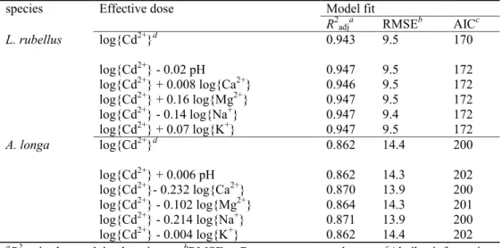
where the coefficients α (= nH/nCu), βi (= nCi/nCu), and γ are constants. Stepwise multiple linear regression analysis was carried out using SPSS 16.0 (IBM) to decide which toxicity-modifying factors (H+_{, Na}+_{, Ca}2+_{, Mg}2+_{, and K}+_{) need to be included in the model. This} model was further applied to predict Cu toxicity to a range of other soil organisms with different endpoints using the underlying data in the literature (Criel et al., 2008; Oorts et al., 2006; Rooney et al., 2006; Thakali et al., 2006a; 2006b).

The general practice in applying the toxicity model to the data is to calculate individual toxic endpoints (LC50 or EC50) for each species in each soil (i.e., point estimates of toxicity), as the best test of a model’s predictive ability is how well it predicts LC50 or EC50 (Thakali et al., 2006a). However, it may also be possible to extend the multicomponent Freundlich model (equation 2-2) to consider the entire dose−response curve. Although γ is constant at a given effect level, it will vary according to the effect level being described. The coefficient α and βi, describing the effects of cations on Cu toxicity, are assumed to be independent of the effect level (Lofts et al., 2004). Generalizing to any effect level, the model reads

log{Cu2+_}

EFFECT = α pH − ∑βi log{Ciz+} + γEFFECT (2-3)

γEFFECT = log{Cu2+}EFFECT − α pH + ∑ βi log{Ciz+} (2-4) here, γEFFECT can be interpreted as the effect dose that incorporates not only the {Cu2+}, but also the terms describing the effects of bioavailability, and differences in inherent sensitivity of organisms to Cu. {Cu2+_}

EFFECT is the corresponding value of {Cu2+} at any given effect

level.

The entire data set for each earthworm species were fitted with a logistic dose−response curve (equation 2-5) (Haanstra et al., 1985) using total Cu concentration, {Cu2+_{}, and γ}

EFFECT as dose, respectively.



) ( 1

50 0

xx R R



 (2-5)

where R = response, R0= control response, x = total Cu concentration, {Cu2+}, and γEFFECT,

x50 = concentration (dose) at the 50% effect level, and β = shape parameter. R was plotted against x to fit the parameters x50 and β. The model parameters were estimated by minimizing the RMSE (root-mean-square error) using the SOLVER program in Microsoft Excel 2010.

2.3 Results and discussion Soil and porewater properties

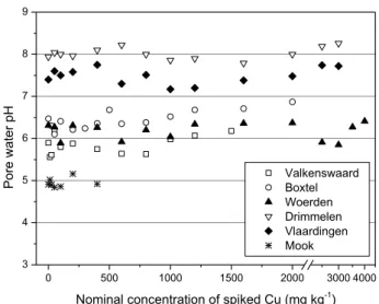
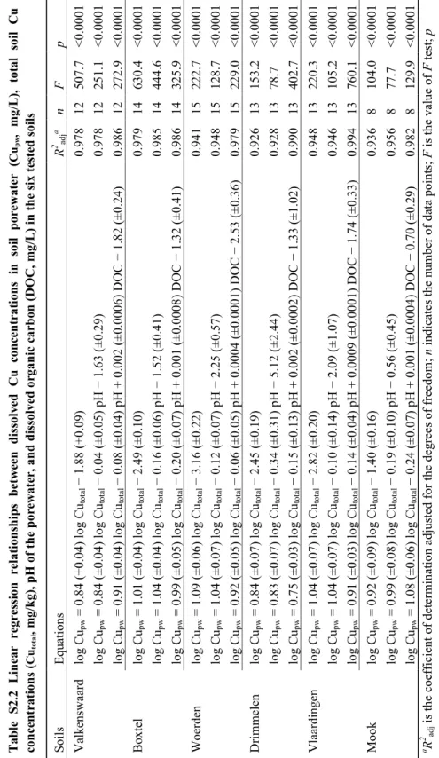
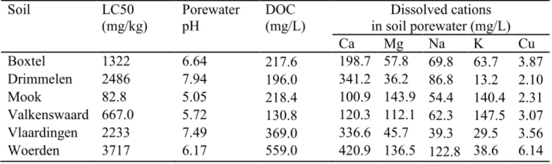
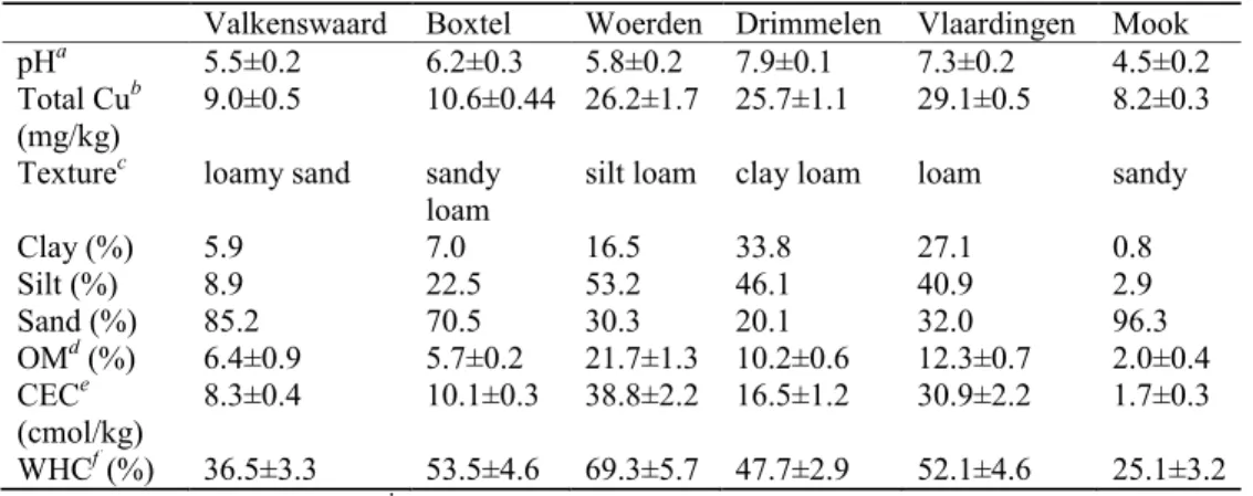
The most important properties of the unspiked soils are presented in Table 2.1. These soils represented a range of soil types and varied in soil pH, OM, and CEC, etc. The selected properties of soil porewater are listed in Table S2.1 in the SI. Soil porewater pH prior to spiking ranged from 5.0 ± 0.2 to 8.0 ± 0.3. The addition of different amounts of Cu (0-4000 mg/kg) only induced marginal effects (usually < 0.3 units) on the soil porewater pH (Figure S2.1 in the SI). It has been reported that the effects of Cu spiking on soil properties can be reduced to a minimum by using Cu acetate instead of other Cu salts (e.g., CuCl2, Cu(NO3)2, and CuSO4) (Qiu et al., 2011). Dissolved Cu concentrations in soil porewater increased with increasing total Cu concentrations. Significant linear relationships between porewater Cu and total Cu were found for all soils (p < 0.0001) (Table S2.2in the SI). The significance of the regression equations was not improved by the inclusion of porewater pH or DOC as explanatory variables.The relationship between calculated and measured pCu (−log{Cu2+_}) in the porewater of all soils is shown in Figure S2.2 in the SI. The free Cu2+ _activities spanned almost 6 orders of magnitude. A significant correlation between calculated and measured pCu was observed (R2 _{= 0.85, n = 75, p < 0.0001, F = 369.6). WHAM VI provided} robust predictions of free Cu2+ _{activities even for the alkaline soils. According to a soil} solid-solution partition model for metals (Lofts et al., 2004), pCu in the porewater of all soils

conformed to a equation: pCu = 0.714pH − 0.211log(total Cu) + 3.565log(OM) + 5.203, (R2

Chapter II

34

Table 2.1 Selected soil properties of the unspiked soils. All values are given as means of three replicates.

Valkenswaard Boxtel Woerden Drimmelen Vlaardingen Mook

pHa _{5.5±0.2 6.2±0.3 5.8±0.2 7.9±0.1 7.3±0.2 4.5±0.2}

Total Cub

(mg/kg) 9.0±0.5 10.6±0.44 26.2±1.7 25.7±1.1 29.1±0.5 8.2±0.3

Texturec _{loamy sand sandy}

loam silt loam clay loam loam sandy

Clay (%) 5.9 7.0 16.5 33.8 27.1 0.8

Silt (%) 8.9 22.5 53.2 46.1 40.9 2.9

Sand (%) 85.2 70.5 30.3 20.1 32.0 96.3

OMd _{(%) 6.4±0.9 5.7±0.2 21.7±1.3 10.2±0.6 12.3±0.7 2.0±0.4}

CECe

(cmol/kg) 8.3±0.4 10.1±0.3 38.8±2.2 16.5±1.2 30.9±2.2 1.7±0.3

WHCf _{(%) 36.5±3.3 53.5±4.6 69.3±5.7 47.7±2.9 52.1±4.6 25.1±3.2}

a_{pH in 0.01M CaCl}

2 extract. baqua regia digestion. cDetermined by the hydrometer method (Pansu and Gautheyrou, 2006). d_{Organic matter content determined by the ignition method}

(Pansu and Gautheyrou, 2006). e_{Cation exchange capacity determined by ammonium acetate}

method (Pansu and Gautheyrou, 2006). f_{Maximum water-holding capacity determined by the}

saturation and gravity drainage method (Pansu and Gautheyrou, 2006).

Entire dose−response relationships

The relationships between survival rate of earthworms and three different expressions of exposure (total Cu concentration, {Cu2+_{}, andγ}

EFFECT) are shown in Figure 2.1. Earthworm

survival rate decreased with increasing total Cu concentrations (Figure 2.1, first column). Copper toxicity to each earthworm species varied widely in the different soils. When expressed as total concentration, LC50 of Cu ranged from 32.4 to 284 mg/kg for L. rubellus, from 39.5 to 1942 mg/kg for A. longa, and from 82.8 to 3717 mg/kg for E. fetida (Table 2.2). Apart from calculating LC50s in six individual soils, an overall LC50 for each species was also obtained by fitting the toxicity data in all soils together with equation 2-5 (Table 2.2). In case of using the total Cu concentration as the expression for Cu toxicity, poor fits were observed with R2 _{of 0.35 and RMSE of 33.9 for L. rubellus, R}2 _{of 0.32 and RMSE of 36.9 for}

A. longa, and R2 _{of 0.27 and RMSE of 33.0 for E. fetida (Figure 2.1, first column). The large}

differences between the individual LC50 values and the overall LC50 values showed that total soil concentration failed to explain the variation in Cu toxicity among soils.

present study confirmed what could be expected: free Cu2+ _{in soil porewater, rather than total} Cu in soil, is the dominant toxic species for earthworms.

0.5 1.0 1.5 2.0 2.5 3.0 3.5 0 20 40 60 80 100 120 Lumbricus rubellus Surviv

al rate (%)

log(total Cu), (mg kg-1₎ R2 _{= 0.35}

RMSE = 33.9

-12 -10 -8 -6 0 20 40 60 80 100 120

R2 _{= 0.79} RMSE = 18.7 Lumbricus rubellus

Surviv

al rate (%)

log{Cu2+_{} (M)}

-12 -10 -8 -6 -4 0 20 40 60 80 100 120 Lumbricus rubellus Surviv

al rate (%)

EFFECT (log{Cu2+} (M) + 0.14pH) R2 _{= 0.87}

RMSE = 15.8

0.5 1.0 1.5 2.0 2.5 3.0 3.5 0 20 40 60 80 100 120 Aporrectodea longa Surviv

al rate (%)

log(total Cu) (mg kg-1₎ R2 _{= 0.32}

RMSE = 36.9

-12 -10 -8 -6 -4 0 20 40 60 80 100 120

R2 _{= 0.89} RMSE = 14.1 Aporrectodea longa

Surviv

al rate (%)

log{Cu2+_{} (M)}

-12 -10 -8 -6 -4 0 20 40 60 80 100 120 Aporrectodea longa

R2 _{= 0.95} RMSE = 9.8

Surviv

al rate (%)

 EFFECT (log{Cu2+} (M) + 0.12pH)

0.5 1.0 1.5 2.0 2.5 3.0 3.5 4.0 0 20 40 60 80 100 120 Eisenia fetida Surviv

al rate (%)

log(total Cu) (mg kg-1₎ R2 _{= 0.27}

RMSE = 33.0

-12 -11 -10 -9 -8 -7 -6 -5 -4 0 20 40 60 80 100 120 Surviv

al rate (%)

log{Cu2+_{} (M)} Eisenia fetida

R2 _{= 0.57} RMSE = 25.9

-8 -7 -6 -5 -4 -3 -2 -1 0 0 20 40 60 80 100 120 Surviv

al rate (%)

EFFECT (log{Cu2+} (M) + 0.66pH) Eisenia fetida

R2 _{= 0.88} RMSE = 13.4

Figure 2.1 Dose−response relationships between survival rate and total Cu

concentration in soil (first column), free Cu2+ _{activity in soil porewater (second column),}

effect dose γEFFECT (third column) for the earthworms Lumbricus rubellus, Aporrectodea

longa, and Eisenia fetida in all six tested soils after 28 days of exposure. The solid lines represent the log-logistic model fits (equation 2-5). R2 _{indicates the coefficient of}

Chapt er II 36 Tab le 2.2 M ed ian let hal con ce ntr at ion s of Cu exp re ssed as tot al Cu c on ce ntr at ion s (L C5 0[C u], (m g/ kg) ) an d fr ee Cu

2+ ac

tivitie s (L C50 {Cu 2+ }, (M )) for th e ear thw or m s Lum bri cu s ru be llu s , A porrec todea lon ga , an d Ei se nia fe tida e xp osed in d iff er en t soil s f or 28 days ( n = 3) . a Indivi dua l L C50 fo r e ac h spe

cies in e

ac h soi l wa s ca lcula ted usin

g the tr

imm ed Spe arma n-K arbe

r method (

Ha

mi

lton

e

t al., 1977

). T he ove ra ll LC 50 fo r e ac h spe cies w as obt ained b y f itti ng the tox icit y da

ta in a

ll teste d soil s tog ether with a lo gi sti c d ose -re sponse c ur ve (e qua tion 2-5) . b 95% co nf idenc e i nt er val s.

c Not

ap pl ica bl e Soil s LC 50 [C u] a for L . rube llus log LC 50 {C u 2+ } for L . rube llus LC 50 [C u] for A. longa log LC 50 {C u 2+ } for A. longa LC 50 [C u] for E. fe tida log LC 50 {C u 2+ } for E. fe tida Box tel

72.2 (64.7

~80.4) b -8.65 (-8.52~ -8.80) 111.1 (80.2 ~153.9)

-7.89 (-7.42~

-8.17) 1322 (1033 ~1692) -6.14 (-5.89~ -6.31) Dr im mele n

279.2 (193.

8~

402.2)

-8.94 (-8.82~9.22) 753.2 (559.

2~

1014)

-8.37 (-8.18~

-8.52) 248 6 (23 90 ~2586)

-7.41 (-7.18~

-7.67)

Mook

32.4 (28.1

~37.3)

-7.69 (-7.50~

-7.83)

39.5 (34.9

~44.7)

-6.94 (-6.71~

-7.16)

82.8 (68.5

~100.1)

-5.46 (-5.24~

-5.59)

Va

lkensw

aa

rd

36.1 (30.4

~42.9)

-8.09 (-7.91~

-8.23)

156.8 (142.

5~

172.5)

-7.12 (-6.84~

-7.43)

667.0 (574.

5~

774.4)

-5.56 (-5.33~

-5.72)

Vla

ardin

ge

n

238.3 (162.

9~

348.6)

-9.30 (-9.11~

-9.42)

618.0 (548.

9~

695.7)

-8.44 (-8.12~

-8.70) 223 3 (214 4~ 232 6)

-7.13 (-7.01~

-7.38)

W

oe

rde

n

283.6 (208.

4~

385.8)

-8.36 (-8.25~

-8.62)

194

2

(1779

~2119)

-7.68 (-7.34~

-7.81) 371 7 (367 8~ 3756)

-6.05 (-5.85~