(will be inserted by the editor)
Scatterplot Layout for High-dimensional Data
Visualization
Yunzhu Zheng · Haruka Suematsu · Takayuki Itoh · Ryohei Fujimaki · Satoshi Morinaga · Yoshinobu Kawahara
Received: date / Accepted: date
Abstract Multi-dimensional data visualization is an important research topic that has been receiving increasing attention. Several techniques that apply scat-terplot matrices have been proposed to represent multi-dimensional data as a collection of two-dimensional data visualization spaces. Typically, when using the scatterplot-based approach it is easier to understand relations between particu-lar pairs of dimensions, but it often requires too particu-large display spaces to display all possible scatterplots. This paper presents a technique to display meaningful sets of scatterplots generated from high-dimensional datasets. Our technique first evalu-ates all possible scatterplots generated from high-dimensional datasets, and selects meaningful sets. It then calculates the similarity between arbitrary pairs of the se-lected scatterplots, and places relevant scatterplots closer together in the display space while they never overlap each other. This design policy makes users easier to visually compare relevant sets of scatterplots. This paper presents algorithms to place the scatterplots by the combination of ideal position calculation and rectan-gle packing algorithms, and two examples demonstrating the effectiveness of the presented technique.
Keywords Visualization· Scatterplot·Isomap· Force-directed graph layout· Rectangle packing
1 Introduction
Multi-dimensional data visualization is an important and active research field. According to survey papers in the field, several techniques have been proposed [Wong 97, Grinstein 01]. The authors of [Wong 97] divided the available multi-dimensional data visualization techniques into three categories: two-variate dis-plays, multivariate disdis-plays, and animation.
Yunzhu Zheng, Haruka Suematsu, Takayuki Itoh
Department of Information Sciences, Ochanomizu University 2-1-1 Otsuka, Bunkyo-ku, Tokyo 112-8610 Japan
The typical two-variate display technique is the scatterplot, which assigns two of the dimensions onto the X- and Y-axis of the two-dimensional display space. Because historically scatterplots have been widely used and are currently imple-mented in commercial spreadsheet software packages, they are particularly popular and users are familiar with them. The scatterplot matrix, which consists of mul-tiple adjacent scatterplots, has also been widely used to represent the dimensions of high-dimensional datasets. Each scatterplot is identified by its row and column index. Even though ordinary users are familiar with scatterplot matrix, they have two major drawbacks. First, if the number of dimensions in a given dataset is very large, the individual scatterplots in a display space may be very small. Second, it is difficult to visually compare arbitrary pairs of scatterplots that are distantly placed in the display space.
Multivariate display techniques attempt to represent the distribution of all the dimensions in a given dataset on a single display space. Several multivariate display techniques are available, including icon- and glyph-based techniques, such as hier-archical axis [Mihalisin 90], worlds within worlds [Feiner 90], parallel coordinates [Inselberg 90], VisDB system [Keim 94], and XmdvTool [Ward 94]. Recently, the parallel coordinates technique has been the subject of many studies and is widely used. However, this technique has several drawbacks. First, when the number of dimensions is very large it may require a large horizontal display space. Second, it is difficult to represent the correlation of a particular dimension with three or more dimensions.
In this paper, we present a technique to represent high-dimensional spaces using multiple scatterplots. Our proposed technique overcomes the drawbacks of both the two-variate and multi-variate data visualization techniques. The proposed technique selectively displays meaningful sets of scatterplots. Our technique first selects a pre-defined number of scatterplots based on a particular conditions. Here, we think one of the meaningfulness of the scatterplots can be determined based on separateness of particular classes, and therefore the separateness is applied as the condition in this paper. Then, it defines the distances or connectivity between all the pairs of scatterplots. Next, it computes the ideal positions of the scatterplots based on their distance or connectivity values. Finally, it applies a rectangle pack-ing algorithm and places the scatterplots [Itoh 06] [Itoh 09] based on their ideal positions. By the combination of ideal position calculation and rectangle packing algorithms, our technique places similarly looking scatterplots closer together in the display spaces, while they never overlap each other.
This paper presents visualization results two example datasets demonstrating the effectiveness of the presented technique.
2 Related Work
2.1 Scaterplot
As discussed in Section 1, many scatterplot-based techniques use dimension re-duction or the scatterplot matrix. Dimension rere-duction is useful in representing in a single display space, the overall distribution of vectors in multidimensional spaces. The effectiveness of dimension reduction depends strongly on the projec-tion scheme selected. Leban et al. [Leban 05] introduced VisRank, which supports
users in obtaining meaningful projections. Scaterplot matrix is often preferable because it directly assigns dimensions to the axes of scatterplots. However, these techniques have the drawback that the size of the scatterplots displayed may be very small.
To address the problem, Wilkinson et al. [Wilkinson 05] and Sips et al. [Sips 09] presented techniques emphasizing on displaying meaningful scatterplots. How-ever, because these techniques are still based on matrix-based layouts of scat-terplots, it is often difficult to effectively represent correlations among scatter-plots. Developing interactive mechanism is another approach for exploration of high-dimensional spaces. Recently, various interactive techniques, such as rolling the dice [Elmqvist 08], have been introduced to assist users in exploring high-dimensional spaces.
2.2 Rectangle Packing
Our proposed technique applies a rectangle packing algorithm to visualize hierar-chical data [Itoh 06]. The rectangle packing algorithm represents a hierarchy as nested rectangles and leaf-nodes as painted icons. Moreover, it mostly satisfies the following conditions:
Condition 1: It never overlap the leaf-nodes and branch-nodes in a single hierarchy of other nodes.
Condition 2: It minimizes the display area.
Condition 3: It minimizes the aspect ratio and area of the rectangular subspaces. Condition 4: It minimizes the distances between the actual and ideal positions of the rectangular subspaces (when the ideal positions of the rectangular sub-spaces are provided).
First, the rectangle-packing algorithm specifies the order of the placement of rect-angles. Then, it identifies several candidate positions that satisfy condition 1, for placing a rectangle. Next, for each candidate position, it computes penalty val-ues, which represent to what extent each position satisfies conditions 2, 3, and 4, respectively. Finally, it places the rectangle at the best candidate position.
This rectangle packing algorithm has also been applied to a graph visualization technique [Itoh 09]. The technique first applies hierarchical clustering to a given graph, and generates clusters of nodes based on both their assigned categories and connectivity. Then, it visualizes the hierarchy by applying a hybrid force-directed and space-filling layout. The force-directed layout minimizes distances between connected or similarly categorized nodes. Conversely, the space-filling layout ap-plies the rectangle-packing algorithm to minimize the cluttering of nodes and max-imize the utility of the display. Hence, the hybrid layout for graph visualization realizes simultaneously both features.
3 Scatterplot Packing for High-Dimensional Data Visualization
This section firstly defines the input datasets and outputs, and briefly describes the processing flow of the scatterplot packing. It then presents in detail how we implement high-dimensional data visualization by packing a set of scatterplots.
Our implementation firstly selects a set of meaningful scatterplots. Next, it com-putes their ideal positions based on their similarity values. Finally, it applies the rectangle packing algorithm to adjust the positions of the meaningful scatterplots.
3.1 Data structure
In this paper, ann-dimensional input datasetDsis defined as follows:
Ds={x1, ..., xN}, (1)
where xi is thei-th vector, and N is the number of vectors. Our technique first forms pairs of thendimensions:
Gp={g1, ..., gG}, gi ={di1, di2}, (2) wheregiis thei-th pair of the dimensions,G=n(n−1)/2 is the number of pairs, anddij is thej-th dimension ofgi.
3.2 Processing flow
Our proposed technique first constructs a set of two-dimensional datasets from the high-dimensional input dataset. Let Si = {xd1i, ..., xdNi} be a set of scalar values, where xdi
j is the value of the di-th dimension of the j-th vector. Our technique compares arbitrary pairs of valuesSi andSj, and if they are similar or correlative, categorizes thei-th andj-th dimensions into the same group. Next, it computes the similarities or distances between arbitrary pairs of values of the datasetsDpi and Dpj. Here, the dataset Dpi = {x1, ..., xN} is a dataset consisting of two-dimensional vectors constructed by extracting an arbitrary pair of dimensionsgi fromDs. Finally, it calculates the positions of the two-dimensional datasets and places similar ones closer together in the display space.
Our technique first calculates the ideal positions of the scatterplots, and then applies the rectangle packing algorithm to adjust their positions. This two-step technique satisfies the following requirements: (1) it places similar scatterplots closer together in the display space, and (2) it avoids overlaps, thus reducing wasted space in the display regions.
Our current implementation of computing ideal positions supports the follow-ing two methods:
– Dimension reduction based on the similarity distances between scatterplots.
– Graph layout, where scatterplots are connected based on their similarity mea-sures.
3.3 Selection of Scatterplots
As mentioned above, our approach first selects a set of meaningful scatterplots. We assume that one of the classes,{Y1, ..., YC}, is assigned exclusively to the vectors of a multidimensional dataset. Here,C is the number of classes, andYjis thej-th constant value which denotes a particular class. Our current implementation selects
a set of scatterplots which have the particular features that vectors of particular classes are well-separated from other vectors. This section proposes formula for determining class separation and an algorithm to select the scatterplots.
First, we compute the entropyHallfor all pairs of dimensions
Hall(gk) =−1/N N n=1 C c=1 p(yn=c|xgnk) logp(yn=c|xgnk) (3) wherexi is thei-th vector,yi is the class assigned to the i-th vector, andp(yn=
c|xgk
n) is the probability that thec-th classYcis assigned to then-th vectorxn. Moreover,xgij is a two-dimensional vector containing the k-th pair of the di-mensions of xi. This value represents the separation of classes in a scatterplot generated by the k-th pair of the dimensions. Furthermore, we compute the en-tropyHcwith thec-th class, for all classes (1≤c≤C).
Hc(gk) =−1/N N n=1 p(yn=c|xgnk) logp(yn=c|xgnk) +p(yn=c|xgnk) logp(yn=c|xgnk) (4) This value represents the separation of thec-th class from other classes in a scat-terplot generated by thek-th pair of the dimensions.
Our implementation first computesHallandHcfor all pairs of dimensions as shown in Figure 1(1). Next, it selects a predefined number of pairs of dimensions which have the smallerHall and/orHcvalues. ValuesHall andHcare also used in Section 3.4 to place similarly looking scatterplots closer together in the display space. (1) Entropy calculation d1 dn d1 dn Calculate(Hall, H1, …, HC)
for all pairs of dimensions
(2) Distance matrix of scatterpots
S1 S1
Calculate distances between pairs of the vectors (Hall, H1, …, HC)
Dimension pairs selection
(3) Ideal position calculation
S1 S2 S3 S4 (4) Scatterplot packing S1 S2 S4 S3 By dimension reduction or force-directed graph layout Fig. 1 Illustration of selecting and placing scatterplots.
Though this section introduces a scatterplot selection algorithm based on class separation, there are other meaningful metrics. For example, centrality [Correa 12] may be a good criterion for scatterplot selection.
3.4 Placement of Selected Scatterplots
In this subsection, we describe how the selected set of scatterplots is placed onto the display space. Our technique first computes the ideal positions of the scatterplots on the display space based on their similarity, and then adjusts their positions by a rectangle packing algorithm. We prepare two algorithms for the ideal position computation which are alternatively applied.
3.4.1 Dimension reduction for computing ideal positions
The entropy values Hall, H1, ..., HC are arranged in a C+ 1 dimensional vector, termed the “entropy vector” of the section. Here, the section denotes the number of scatterplotsM, the number of dimensions of the entropy vectorsdim=C+ 1, and the entropy vector of thej-th scatterplotSj. Next, we calculate the similarity distances between thea-th andb-th scatterplots, and generate anM×M matrix containing the distances of all possible pairs of scatterplots, as shown in Figure 1(2). Then, we apply to the matrix the Isomap scheme and compute the two-dimensional positions of the scatterplots.
3.4.2 Graph layout for computing ideal positions
Instead of generating a distance matrix, we generate a graph structure by con-necting pairs of scatterplots that are sufficiently similar. Next, we apply a force-directed graph layout technique and compute the two-dimensional positions of the scatterplots. Our implementation simply sets the stable lengths of edges as the above mentioned similarity distance values before applying the force-directed lay-out, while it does not consider the sizes of nodes. This process can be improved by applying more sophisticated techniques [Harel 02] [Lin 09].
3.4.3 Rectangle packing
After calculating the ideal positions of the scatterplots by selectively applying di-mension reduction or graph layout techniques, as shown in Figure 1(3), we compute the final positions of the scatterplots by applying a rectangle packing algorithm, as shown in Figure 1(4).
4 Example
In this section, we present examples of visualizing datasets using our technique described above. We implemented in Python 2.7 the scatterplot selection (Section 3.3), and dimension reduction (Sections 3.4.1) algorithms. Moreover, we imple-mented the force-directed layout (Sections 3.4.2) and rectangle packing (Sections 3.4.3) algorithms using the Java Development Kit (JDK) 1.6.0. We executed the implementation on Lenovo ThinkPad T420s (Intel Core CPU 2.70GHz and 8GB RAM) with 64 bit version of Windows 7 Service Pack 1.
In our experiments, we observed large differences in the quality and computa-tion time between approaches using dimension reduccomputa-tion and force-directed graph
layout. Dimension reduction required approximately ten minutes of computation time, while force-directed graph layout required only several seconds. Conversely, the visualization quality using dimension reduction was subjectively much better. In the next subsection, we present visualization results obtained using dimen-sion reduction.
4.1 Example 1: Image segmentation data
In this subsection, we present the visualization results obtained by applying our technique to the “Segmentation” dataset published at the UCI machine learning repository [Data-seg]. This dataset contains 18 feature values of 210 blocks of images. Here, the blocks are generated by dividing each of 7 images into 30 blocks. We treated images as classes, feature values as dimensions, and blocks as vectors. Hence, the 18-dimensional dataset is displayed as 210 vectors in 7 colors.
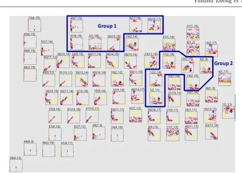
In Figure 2, the technique displays 68 scatterplots resulting from our experi-ment. The figure shows many of scatterplots selected by the presented technique well separate particular classes. Also, the figure shows that the layout of scatter-plots never overlap them while not causing large empty spaces, by the effort of the rectangle packing algorithm. We subjectively defined two groups of similarly looking scatterplots in this figure. This section calls them “Group 1” and “Group 2”. “Group 1” denotes a group of scatterplots for which the red vectors are well separated from vectors with other colors. “Group 2” denotes another group of scat-terplots for which the black vectors are moderately separated from vectors with other colors, in addition to the yellow and red vectors. This result demonstrates the presented technique well gathers scatterplots which the same classes are well separated closer in the display space.
Figure 3 shows a close-up view of the six scatterplots belonging to “Group 2.” In addition, this figure demonstrates that our technique performs well in grouping similarly looking scatterplots closer together in the display space. In Figure 3, the two-dimensional values displayed above the scatterplots indicate the IDs of the dimensions assigned to the two axes of the scatterplots. The second values of the six pairs of dimensions indicate the following [Data-seg]:
9: Average of (R + G + B)/3 value over the region. 10: Average of the R value over the region.
15: Average of the (2B - (G + R)) value over the region.
16: 3D nonlinear transformation of the RGB values using the algorithm of Foley and VanDam.
Here, R, G, and B are red, green, and blue components of the pixel values. These results demonstrate that the variables of the three images (visualized as yellow, red, and black vectors) are characteristic and similarly distributed.
The vectors displayed in Figure 4 (Left) represent the ideal positions of the scatterplots calculated using the Isomap scheme. Similarly, the vectors displayed in Figure 4 (Right) represent the final positions of the scatterplots shown in Figure 2. We subjectively made seven groups of vectors indicated as (1) to (7) to observe their movements by the rectangle packing process. Figure 4 demonstrates that vectors in these groups remain adjacent. Moreover, the figure indicates that the scatterplots displayed in Figure 2 do not overlap and there are no unnecessary gaps in the display space.
Group 1
Group 2
Fig. 2 Visualization of an image segmentation dataset as 68 scatterplots.
Fig. 3 Close-up view of the six scatterplots belonging to “Group 2” shown in Figure 2.
4.2 Example 2: Vehicle specification data
In this subsection, we present visualization results obtained by applying our ap-proach to a vehicle specification dataset constructed from websites containing on-line vehicle catalogs [Data-veh]. This dataset contains 70 feature values and various classes for 429 vehicles. Hence, the 70-dimensional dataset is displayed as 429 vectors. Here, the feature values include sales-related values such as price, performance-related values such as displacement and fuel efficiency, and size-related values such as width and length. In addition, this dataset contains var-ious average values of 5-point subjective user evaluations, including appearance, equipment, interior, engine power, cost performance, and the total.
We divided the vehicles according to the range of one of the average evaluation values listed above, and colored the vectors according to the corresponding range of evaluation values.
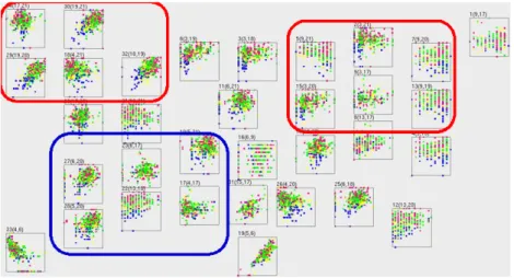
In Figure 5, we present the set of scatterplots obtained by applying our tech-nique to the vehicle specification dataset. Here, the colors of the vectors denote ranges of appearance evaluation values. Vehicles with the highest appearance
eval-(1) (2) (3) (1) (2) (3) (4) (4) (5) (5) (6) (6) (7) (7)
Fig. 4 (Left) Ideal positions of scatterplots calculated by the Isomap scheme. (Right) Final positions of scatterplots shown in Figure 2.
Fig. 5 Visualization of a vehicle specification dataset using scatterplots. Colors of vectors denote appearance evaluation.
uation values are drawn in pink. We use red rectangles to indicate scatterplots containing pink vectors that are well-separated from vectors with other colors. Several of these scatterplots assign multiple common variables to their axes, such as height of floor, evaluation of equipment, interior, cost performance, and total. This result suggests that the height of floor is one of the most important specifica-tion values correlated to the impression of appearance of vehicles. In addispecifica-tion, it suggests that appearance evaluation is well correlated to other evaluation values. Several of the scatterplots that are not well separated from the pink vectors are indicated by a blue rectangle. Several of these scatterplots assign multiple common variables to their axes, such as outer length, outer height, and outer width. An unexpected result obtained is that the values of the outer size of a vehicle did not have a major correlation to its appearance evaluation.
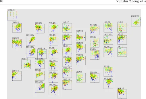
In Figure 6, we present another visualization example using a set of scatter-plots. Here, the colors of vectors denote ranges of values of cost performance evalu-ation. In several scatterplots, vehicles those cost performance are highly evaluated
Fig. 6 Visualization of a vehicle specification dataset using scatterplot. Colors of vectors denote cost performance evaluation.
(drawn in pink) are well-separated from vehicles those cost performance are poorly evaluated (drawn in blue). Several of the scatterplots assign multiple common vari-ables to their axes, such as appearance and total evaluations. This result suggests that the evaluation of appearance strongly correlates to the cost performance and total evaluation.
The two figure show that the layout of scatterplots never overlap them while not causing large empty spaces, by the effort of the rectangle packing algorithm.
5 Conclusion
In this paper, we presented a technique for visualizing high-dimensional data as a set of well-selected and arranged scatterplots. Our technique first selects meaning-ful pairs of dimensions, and computes the similarity between arbitrary pairs of the dimension pairs. It then calculates the ideal positions of scatterplots representing the dimension pairs based on their similarity distances, and finally adjusts their positionsby a rectangle packing algorithm. We presented examples of applying our proposed technique to visualize image segmentation and vehicle specification datasets.
As a future work, we would like to perform additional experiments in various applications. Specifically, we would like to apply our technique to larger datasets containing hundreds of dimensions and tens of thousands of vectors to demonstrate its scalability. In addition, we would like to apply our technique to various fields of datasets to demonstrate its usability as a generic visual analytics tool. Meanwhile, we also would like to numerically and subjectively evaluate our technique. For example, we would like to compare the distances among the scatterplots on the display space with their similarity distances.
References
[Correa 12] C. D. Correa, T. Crnovrsanin, K.-L. Ma, Visual Reasoning about Social Networks Using Centrality Sensitivity.IEEE Transactions on Visualization and Computer Graphics, 18(1), 106-120, 2012.
[Elmqvist 08] N. Elmqvist, P. Dragicevic, J. Fekete, Rolling the Dice: Multidimensional Visual Exploration using Scatterplot Matrix Navigation,IEEE transactions on Visualization and Computer Graphics, 14(6), 1141-1148, 2008.
[Feiner 90] S. Feiner, C.Beschers, Worlds within Worlds: Metaphors for Exploring n-dimensional Virtual Worlds,ACM Symposium on User Interface Software and Technology (UIST ’90), 76-83, 1990.
[Grinstein 01] G. Grinstein, M. Trutschl, U. Cvek, High-Dimensional Visualizations, KDD Workshop on Visual Data Mining, 2001.
[Harel 02] D. Harel, Y. Koren, Drawing Graphs with Nonuniform Vertices,Advanced Visual Interfaces (AVI) 2002, 157-166, 2002.
[Inselberg 90] A. Inselberg, B. Dimsdale: Parallel Coordinate: A Tool for Visualizing Multi-Dimensional Geometry,IEEE Visualization, 361-370, 1990.
[Itoh 06] T. Itoh, H. Takakura, A. Sawada, K. Koyamada, Hierarchical Visualization of Net-work Intrusion Detection Data in the IP Address Space,IEEE Computer Graphics and Applications, 26(2), 40-47, 2006.
[Itoh 09] T. Itoh, C. Muelder, K. Ma, J. Sese, A Hybrid Space-Filling and Force-Directed Layout Method for Visualizing Multiple-Category Graphs, IEEE Pacific Visualization Symposium, 121-128, 2009.
[Keim 94] D. A. Keim, H.-P. Kriegel, VisDB: Database Eploration Usng Multidimensional Visualization,IEEE Computer Graphics and Applications, 14(5), 40-49, 1994.
[Leban 05] G. Leban, I. Bratko, U. Petrovics, T. Curk, B. Zupan, VizRank: Finding Infor-mative Data Projections in Functional Genomics by Machine Learning, Bioinformatics Applications Note, 21(3), 413-414, 2005.
[Lin 09] C. Lin, H. Yen, J. Chuang, Drawing Graphs with Nonuniform Nodes Using Potential Fields,Journal of Visual Languages and Computing, 20(6), 385-402, 2009.
[Mihalisin 90] T. Mihalisin, E. Gawlinski, J. Timlin, J. Schwegler, Visualizing a Scalar Field on an n-dimensional Lattice,IEEE Visualization, 255-262, 1990.
[Sips 09] M. Sips, Selecting Good Views of High-Dimensional Data Using Class Consistency?C
Eurographics/IEEE-VGTC Symposium on Visualization, 831-838, 2009.
[Ward 94] M. O. Ward, XmdvTool: Integrating Multiple Methods for Visualizing Multivariate Data,IEEE Visualization, 326-336, 1994.
[Wilkinson 05] L. Wilkinson, A. Anand, R. Grossman, Graph-Theoretic Scagnostics, IEEE Symposium on Information Visualization, 157-164, 2005.
[Wong 97] P. C. Wong, R. D. Bergeron, 30 Years of Multidimensional Multivariate Visualiza-tion, Scientific Visualization: Overviews Methodologies and Techniques,IEEE Computer Society Press, 3-33, 1997.
[Data-seg] UCI Machine Learning Repository, Image Segmentation Data Set, http://archive.ics.uci.e.,du/ml/datasets/Image+Segmentation