A PARALLEL ARCHITECTURE FOR CURVE-EVOLUTION PARTIAL DIFFERENTIAL EQUATIONS

Image Anal Stereol 2003;22:121-132 Original Research Paper

A PARALLEL ARCHITECTURE FOR CURVE-EVOLUTION

PARTIAL DIFFERENTIAL EQUATIONS

E

D

P

D

School of Mines of Paris, Center of Mathematical Morphology, 35, Rue Saint Honoré, 77 300 Fontainebleau, France

e-mail: {dejnozke,dokladal}@cmm.ensmp.fr

(Accepted May 20, 2003)

ABSTRACT

The computation of the distance function is a crucial and limiting element in many applications of image processing. This is particularly true for the PDE-based methods, where the distance is used to compute various geometric properties of the travelling curve. Massive Marchinga_{is a parallel algorithm computing the distance}

function by propagating the solution from the sources and permitting simultaneous spreading of component labels in the influence zones. Its hardware implementation is conceivable as no sorted data structures are used. The feasibility is demonstrated here on a set of parallely-operating Processing Units arranged in a linear array. The text concludes by a study of the accuracy and the implementation cost.

Keywords: distance function, hardware for image processing, partial differential equations, parallel computing.

a_{Short preliminary study published in: Dejnožková and Dokládal (2003b) (algorithm) and Dejnožková and Dokládal} (2003a) (architecture)

INTRODUCTION

Recently, the image processing methods based on Partial Differential Equations (PDE) have gotten an ever increasing attention. The examples of application can be found in numerous domains such as filtering (non-linear diffusion), active contours used for segmentation of either static images (Voronoï graph, watershed, shortest path, object detection) or sequences (object tracking) or more recent methods as shape from shading. The implementation of the PDE-based method requires the computation of non-linear functions. They are often solved by iterative and recursive algorithms characterized by a high computational cost. Therefore, only a limited number of real-time applications exists. The most common existing custom chips implement non-linear filtering,

i.e. the non-linear diffusion (Perona and Malik, 1988; Gijbels et al., 1994). One can find some experiments with super-computers (Sethian, 1996) or some examples of PDE-based segmentation using the level-sets implemented on graphic hardware (Rumpf and Strzodka, 2001).

The design of a custom chip becomes meaningful not only for the acceleration but also for the implementability on embedded systems (Suri et al., 2002). Many authors put forth a considerable effort to reformulate existing sequential algorithms in a parallel form or to speed up the convergence (Weickertet al., 1998). However the number of necessary iterations remains excessively high.

The motivation of our work is to define a general type of parallel architecture fitting the needs of the above-mentioned applications. There are several reasons why few architecture propositions have been made for interface (curve-based) algorithms. The curve traveling in a continuous space n _{is implicitly}

described in a discrete space

n_{by the distance to the}

curve, as proposed first in Osher and Sethian (1988). The distance function is the computation support of the level-set methods. Its zero-level set represents the traveling interface. Its accurate computation is very important because its geometrical properties (e.g. the curvature) are then used to describe its evolution in the time. The interface evolution imposes frequent and random memory accesses. Also, the numerical solution of a classical variational formulation leads to deformations of the implicit description of the curve (Kimmel, 1995) imposing more or less frequent reinitializations. In the work of Zhaoet al.(1996) and Gomez and Faugeras (1992) can be found propositions of algorithm without re-initialization paid by the necessity to search the propagation speed on the zero-level set even for the points situated elsewhere. Because of the complexity and high computational cost, the classical re-initialization approach is still leading (Paragios, 2000). Repetitive re-initialization alternated with another type of processing increases the requirements on the implementing architecture.

of 3D surfaces, minimal path search (Kimmel and Sethian, 2001) or continuous watershed (Meyer and Maragos, 1999).

In Gijbelset al.(1994) has been proposed a linear-array, SIMD architecture for PDE-based filtering by linear diffusion. An efficient hardware (parallel) implementation of a (weighted) distance function preserving the accuracy and the necessary sub-pixel precision for the continuous interface evolution is still needed. The goal of this paper is to show that the same architecture type can also be used for interface evolution algorithms.

This paper is organized as follows. After a brief review of existing distance computing algorithms, we analyse the principles of the Massive Marching. Section “Hardware implementation” presents its hardware implementation. Experiment results state the achieved implementation parameters such as the surface requirements, clock rate and necessary fixed-point precision for a given error.

REVIEW OF EXISTING ALGORITHMS The sub-pixel accuracy is one of the essential features required from algorithms computing the distance function for the level-set methods. The initial condition, a closed curve 0 placed arbitrarily in

n_,

represents the zero-level set of the searched distance functionuxy . Forn 2 we have:

0 xy

2

uxy 0 (1)

Recall that u is discrete, i.e. only ui j i j

2 _is known. Other necessary characteristics required from the distance computing algorithms are the preservation of the accuracy, computation on a narrow band for the active contours and simultaneous propagation of components labels.

Current algorithms used to find u given 0 are

from the hardware implementation aspect optimal only for a particular type of applications. Two types of algorithms exist: the first type proceeds by scanning the entire image and the second type propagates a narrow-band solution from the initial interface.

The algorithms using successive scannings are simple to implement. However, they suffer from a serious drawback that the next scan cannot begin before the previous one ends. Therefore, the scanning-based methods are optimal only for those applications where the solution on the entire image is required. A classical example is the algorithm of Danielsson (1980) which is based on two coordinates description and its overall complexity is N , where N is the

number of points in the image. It yields the square

of the distance function, which imposes to compute the square roots before the distance can be used for other computation, e.g. the curvature. Moreover, this algorithm is not conceived to operate with a sub-pixel precision. This problem is resolved in Tsai (2000) which proposes asweeping algorithm (inspired from Boué and Dupuis (1999)). By using a new numerical scheme, it yields the exact distance and not the square and it reduces the numerical error of the classical Godunov scheme. The complexity of this algorithm is

MN where Mis the number of data points and N

is the number of grid points. However it is not possible to calculate the influence zones of different sources.

The algorithms operating in the narrow band are more appropriate for the propagation of labels. Their implementation is complicated by using sophisticated data structures and the complexity isNlogN. The

Fast Marching introduced by Sethian (1996) is the most often used propagation technique in combination with the PDE-based methods. The algorithm allows to compute the distance function by realizing the principle of Huygens, as it is introduced in Verbeek and Verwer (1990), by propagating equidistant waves. For this, the Fast Marching algorithm needs to use an ordered data structures with a real-number

priority. In every iteration can be processed only

the point with the highest priority. The maximum priority represents a global information and makes this algorithm sequential. Moreover, the hardware implementation of data structures using a real-number priority is difficult because of operations like insertion, reading and re-positioning of elements.

This is not the case of the USP algorithm (Eggers, 1997) which does not use any sorted data structures. However, the result it yields is the square of the distance and it requires to memorize the current iteration number. It does not operate in sub-pixel accuracy and the complexity is n

3

for images of

n npoints.

IMPLEMENTATION ISSUES

The filtering as well as the segmentation algorithms respond to some function of geometrical properties of the level-set functionusuch as gradient or curvature. These geometrical properties are obtained directly from the values of u or its derivatives (Sethian, 1996; Sapiro, 2000). The computation of the derivatives is an elementary operation. For every point concerned, these operations are performed on the nearest neighborhood and are independent each of the other. Hence they can be executed in parallel (Dejnožková, 2002).

Image Anal Stereol 2003;22:121-132

operations, the SIMD (Single Instruction Multiple Data Stream) architecture is the natural choice to reduce the processing time. We propose a divide-and-conquer approach in order to obtain a more balanced processors’ activity and to limit the space on the chip. Thus one can benefit from a quasi parallel implementation by dividing the input data into blocks. Recall that the SIMD architecture consists in an array of processors with an interconnection network for the communication. Each processor has its private non-shared memory. A single controller broadcasts instructions to all the processors. The processors then execute the instructions simultaneously at a given time. The choice of the algorithm to implement and the architecture type come together. Compared to the filtering, other techniques as the continuous watershed or active contours require computation of a (weighted) distance to the given markers. These algorithms use sophisticated ordered data structures (such as hierarchical queues or a sorted heap) which can penalize the execution time on the SIMD architectures. The processing of such data structures introduces a sequential approach. Only one point (with maximal priority) can be processed at a time. Another reason why the SIMD architecture would be less efficient for this type of algorithms is the random access to the memory.

In the next section we show the implementation of the Massive Marching algorithm used for the computation of a distance function. This algorithm is fully parallel. Hence the execution time on an architecture withPprocessors istparallel tsequential

P.

MASSIVE MARCHING

ALGORITHM

Throughout this paper we use the following notations. Let pxpyp

be a point of an isotropic,

rectangular and unit grid. V p denotes the

4-neighborhood of p defined as V pxpyp 1

xp 1

yp

! . The pointqis a neighbor ofpifq

V p ,

u p denotes the value of the distance function inp.

NUMERICAL SCHEME

Numerical schemes allow to obtain the value of the distance function in a point according to the values of the neighbors. The numerical scheme is a discretization of the eikonal equation:

∇u

#"$ (2)

where " is the weight for a weighted distance. Some

propositions of numerical schemes can be found in

Sapiro (2000) or Tsai (2000). The most often used scheme is, in the domain of the Level Set, the scheme proposed by Godunov (Sethian, 1996).

%

max u p'& u(xp 1

yp

)0

2

&

max u p'& u(xpyp 1

0

2*

1 2

+", p- (3)

In order to obtain the maximum values of the terms, we have to consider the neighbors with minimum values ofu. The Godunov scheme requires to determine the maximal real solution of a quadratic equation (3).

Suppose that the distance u in the point p

can be expressed by the following function of the neighborhood V p of the point p and the weight

", p

u p. umin p)/ fdiffV p0", p12 (4)

umin p is the distance value of the minimal neighbor:

umin p3 minq

i4 V

5p6

uqi . The formulation of fdiff

depends on the choice of the numerical scheme. The Godunov scheme can be rewritten in the form of Eq. (4) where fdiffreads as

fdiff

ux p!& uy p

2 /

"7 p

2 2 &98

ux p0& uy p

2 :

2

(5) and whereux p3 min u1xp

1 yp

and uy p;

min u1xpyp 1

In Eq. (5) the minimum real solution is considered. If there is no real solution then the distance value is computed only from the minimal neighbor and fdiff

", p .

INITIALIZATION

0is a closed curve which generally lies between

the points of the grid

2_{. Its accurate inter-pixel} location is identified by the distance map u to 0.

However, if it is to be described implicitly on a discrete support

2_{, the curve}

0 may not be placed

arbitrarily. Its location is determined by the switching function ϕ p where signϕ p1 indicates whether a

given point plies inside or outside 0(as introduced

in Sethian (1996)). Hence, 0 is located between

adjacent points for which signϕ<=1 differs. The exact

distance u of these points to 0 is obtained by some

interpolation method.

less complicated forms (for examples see Osher and Shu (1991); Siddiqi et al. (1997)). The majority of practical applications use a linear approximation. In the following, consider a linear interpolation and

ϕ

const. for all p >

2_{. Since u can only have a finite} number of constant values for all points adjacent to

0, the initialization of the distance function reduces to

u:

2?

c1 c2<<<@cn , where allci . The number

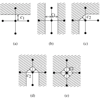
of the constants depends on the number of neighbors from which the interpolation is calculated. The Fig. 1 shows all the possible 4-neighborhood configurations for the linear interpolation.

A A A A A A A A A A A A A A A A A A A A

B B B B B B B B B B B B B B B B B B B B

c1

(a) C C C

C C C C C C C C C C C C C C C C C C C C C C C C C C C

D D D D D D D D D D D D D D D D D D D D D D D D D D D D D D

E E E E E E E E E E E E E E E E E E E E F F F F F F F F F F F F F F F F F F F F c1

(b) G G G G G

G G G G G G G G G G G G G G G G G G G G G G G G G G G G G G G G G G G G G G G G G G G G G

H H H H H H H H H H H H H H H H H H H H H H H H H H H H H H H H H H H H H H H H H H H H H H H H H H

c2

(c)

I I I I I I I I I I I I I I I I I I I I I

J J J J J J J J J J J J J J J J J J J J J

K K K K K K K K K K K K K K K K K K K K K K K K K K K K K K K K K K K K K K K K K K K K K K K K K K

L L L L L L L L L L L L L L L L L L L L L L L L L L L L L L L L L L L L L L L L L L L L L L L L L L

c2

(d) M M M

M M M M M M M M M M M M M M M M M M

N N N N N N N N N N N N N N N N N N N N N

O O O O O O O O O O O O O O O O O O O O O O O O O O O O O O O O O O O O O O O O O O O O O O O O O O

P P P P P P P P P P P P P P P P P P P P P P P P P P P P P P P P P P P P P P P P P P P P P P P P P P

c2

(e)

Fig. 1. Configurations of the 4-neighborhood for the initialization.

If the central point lies on the object’s edge,i.e.the sign of neighbors changes with respect to the central (interpolated) point only in one direction (see Fig. 1(a) or 1(b)), the interpolation is computed only from

ϕ<= of these neighbors. If the sign changes in both

directions (corner or isolated point) the resulting value is computed fromϕQ= of the two neighbors (Fig. 1(c)

to 1(e)).

Hence the initialization of u p can be realized

efficiently as a logical function of signϕ p1

signϕq1R<<1 signϕq4 and the result of the

function is used to retrieve the corresponding value from a look-up-table containing the constantsci.

PROPAGATION

We use the following sets to define the algorithm:

S

is the set of points initialized by the interpolation,

T

is the set of points marked as active T

U qi

qi V

S

andVqi'W

S

V

/0 . The algorithm reads as

follows:

InitializationX

Initialize the neighborhood of the curve with a signed distance (setS

)

X

Initialize the distance value u of the other points to∞

X

Mark the neighbors ofS

asactive(setT

)

Propagation

whileT

V

Y , do in parallel for allp

T

:

Z

Compute new distance valueX :

Jacobi step:

un[ 1

p. u

n

min p1/

min fdiff \V

p]", p1^_`"7 p (6)

X

Gauss-Seidel step:

un[ 1

p. u

n[ 1

min p1/

min fdiff \V

p]", p ^ `"7 pa (7)

Z

Activation of new points to process:X

deletepfromT

, insertpinS

X

ifu p.b NBwidththen for allqi qi V p such

thatun[ 1

qic& u

n[ 1

pd εqi (8)

insertqi ?

T

where NBwidth is the desired width of the narrow band1_{. (The values of unprocessed points in t}

n are

automatically carried over to the next iteration and are noted as values attn[ 1.)

At each iteration, the value is calculated for the

active points. The algorithm does not use any kind

of sorted processing. Consequently, the front of the propagation is not equidistant to the initial curve. Two situations exist where the points that are currently being calculated will have to be reactivated later: 1. The value of the point is calculated on an

incomplete neighborhood which imposes a two-step algorithm

2. The points are activated by a propagation front coming from a source which is not necessarily the closest one which is detected byactivation rule.

1_{To obtainuon the entire image let NB}

Image Anal Stereol 2003;22:121-132

Two-step based algorithm

We say that the point value is computed on an incomplete neighborhood since adjacent (mutually dependent) points may be processed simultaneously. The calculation is therefore performed in two steps. The steps are named after their similarity with the algorithm of Markov chain approximation by PDE as introduced in Boué and Dupuis (1999). The first one,

the Jacobi step, calculates the value of the distance

function attn[ 1 given only the values obtained at tn.

The second one, theGauss-Seidel step, recalculates the distance value attn[ 1by using also the values obtained

attn[ 1.

The algorithm computes the value u p from the

least neighbor. Hence, the infinite values are not considered for the computation. As mentioned above, in the Jacobi iteration, the first estimation of un[ 1

p

is obtained by using the values of neighbors from the previous iteration which is recomputed once more in the Gauss-Seidel step.

Activation rule

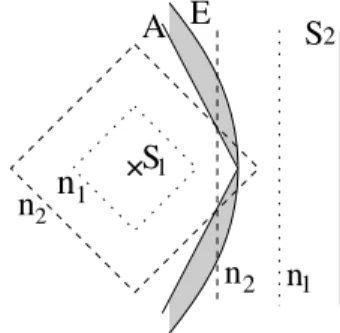
The activation rule has two important roles: the supervision of the propagation end and the detection of the overlapping of the propagation waves (see Fig. 2).

2

n n1 2

S1

2

n

A _S

n

E

Fig. 2.Example of an overlapping of the propagating

waves and zone of reactivation (in gray). S1, S2 are

the propagation sources. The dashed lines represent

the propagation waves after n1and n2iterations.

We calculate the distance function uxf

mindistx S1 distx S2

. Let E denote the set

of points equally distant from S1 and S2, E

x

distx S1g distx S1 . The points to the left

(resp. right) from E are closer to S1 (resp. S2). Note that in this exampleE is a parabola.Adenotes the set of points activated simultaneously by the two fronts coming from the two sources. Since the propagation front of Massive Marching is not equidistant to the propagation source, the setsAandE do not coincide. The zone delimited by A and E contains points that were activated from S2 whereas they are closer toS1. These points will be reactivated again by the front

coming from S1 in order to lower their value from distxS2 to distxS1.

Suppose thatun

p has just been calculated and p

is deactivated. We search for an estimator of un[ 1 qi

to know whether the neighbor qi of p should be

activated in order to compute or to re-compute its value. Since the goal is to obtain the minimal solution the main idea is to test whether the valueuqi could

be brought down by consideringpas the least neighbor ofqi. Suppose that pis the least neighbor ofqi. Then

in the next iteration qi will receive its value from p.

From Eq. (4), fdiff p is the difference between the

distance valueu p of a given point pand the least of

the neighborsumin p . The new valueuqi will satisfy

uqi;h u p)/ inffdiff.

LetKminbe the lower bound of fdiff:

Kmin p. inffdiffV p0", p1. (9)

"7 p is an arbitrary but time invariant function.

Kmin is a predictor of the least increment of u in one iteration. All neighbors qi of p such thatuqi&

u p3d Kmin p should therefore be (re-)activated and

(re-)calculated since the new value u p may affect

uqi in the next iteration. Hence, ε in Eq. (8) must

satisfy:

ε p-h Kmin pd 0

Remark: The lower bound of fdiff of the Godunov scheme (from the section 2.1) is

Kmin pYi

", p

2

2 (10)

Note thatKmin is constant whenever" is constant in

(2) and becomes a function of " whenever" varies

over the image.

Setting ε b Kmin is useless because it would

authorize the activation of points that will not be updated and the propagation could go backwards. By letting ε d Kmin one can authorize fewer

reactivations (lower execution time) paid by some error (proportional to ε& Kmin) in the result (Dejnožková,

2002).

LABEL PROPAGATION

X

Jacobi step

ifux p anduy p have the same label then use Eq.

(6)

else useun[ 1

p u

n

min p)/ F p

X

Gauss-Seidel step

1. ifux p anduyhave the same label use Eq. (6)

else useun[ 1 p u

n[ 1

min p)/ F p

2. preceives the label ofun[ 1 p

COMPUTATION ERROR

Two types of error exist: numerical scheme error and incomplete neighborhood error.

Numerical scheme error

As the majority of first order schemes also the Godunov scheme suffers from “shortsightedness” as it uses only the nearest neighborhood. Moreover, Tsai (2000) explains that when the propagation starts from isolated points it creates diamonds instead of circles. In Sethian (1999) Sethian proposes a switching mechanism between the first and second order scheme in order to improve the accuracy. Nevertheless, in ∞ the Godunov scheme converges to the exact solution.

Incomplete neighborhood error

This error is caused by the computation on an incomplete neighborhood (see section “Two-step based algorithm”). Massive Marching calculates simultaneously the values of adjacent points, i.e.

values depending each on the others. Therefore the calculation is performed in two steps.

Also all the methods referenced in the introduction allow to recalculate the points several times in order to obtain more accurate solution to Eq. (2). The scanning-based methods recalculate during each scanning all the points of the image. Successive scannings have to be repeated until the convergence. Methods for the narrow band use a variable number of recalculations, implemented by using a sorted heap, depending locally on the neighborhood of every particular point. At every recalculation the point receives a new value of the distance according to the new values of the neighbors. Massive Marching authorizes to reactivate the neighborqiif the pointpreceives a new valueu p

inferior touqi`& ε (see condition Eq. 8).

An additive error (typically at the fourth decimal place) may still appear in some special cases (as corners etc.), see Dejnožková (2002). The experiments have shown that the two-step calculation gives sufficient accuracy for most practical applications (see section “Experimental results”). Should more accurate results be required then the Gauss-Seidel step can be repeated.

COMPUTATION COMPLEXITY

In order to obtain the calculation complexity of Massive Marching we first assume that " const.

over the entire image.

The value of an active point p is obtained in a constant time 1 after which the point deactivates

itself. The point activates all its neighbors that verify the condition (8). The function (4) is strictly positive, no point can therefore reactivate the neighbor from which it has received the activation. If the propagation starts from one point representing the source, the algorithm complexity is N , withN be the number

of points in the image.

For sources having more complicated geometrical forms or more than one source the complexity may exceedN since some points may be activated more

than once. We show that the number of reactivations is bounded. Consider two isolated points a and b such that there is a point c, c Va , c Vb and a

V

Vb. Suppose that the two propagation fronts arrive

respectively viaaandband meet inc. The two fronts have different speed and in the iterationnthe distance values in aandb verify

un

a.& u

n

b

h 2Kmin. The

faster front will stop incwhereas the slower one will continue. It can be shown that its propagation will stop afteriiterations, where

i b

un

bc& u

n

a

2Kmin

& 1

In images with"j const., the waves propagate with

unit increment of u in one iteration in vertical and horizontal direction, whereas in the diagonal directions the increment is obtained only after two iterations. See illustration at Fig. 2. The waves arriving fromS1and

S2meet first on the intersection ofAandE since both waves have the same speed on the horizontal direction. Later, see the iterationn2for example, the waves meet outside the skeleton since the wave arriving from S1 arrives diagonally and is therefore slower. The slower wave will continue its propagation up to the skeleton of the distanceEwhere it stops.

For images with bounded support, the term

un

ak& u

n

b

is upper bounded and hence the number of reactivations also. For images where "

V

const.,

this term is also limited and depends on" .

HARDWARE IMPLEMENTATION

Image Anal Stereol 2003;22:121-132

GLOBAL ARCHITECTURE

For the simulation and validation, we have chosen the division of the input image into the columns,i.e.

one processing unit per column of the image. In a given moment the processing units process in parallel all the points in a row. We give below a description of the proposed (and tested) access to the neighbors. The processing units are controlled by the single Global Control block. It reads high-level instructions from the Code Memory. Each high level instruction indicates the action executed on the entire image in one scan and the code does not have to be decomposed in the elementary operations. The algorithm for computing a distance function on the entire image (given in section “Propagation”) resumes to these high-level instructions:

interpolate

loop (if any point is active)

Jacobi_Step

Gauss-Seidel_Step

The conditionany point is activeis the OR operation over all the activation flags.

The Global Control block not only controls the execution of the algorithm but also allows to change the values of the approximation registers inside each processing unit. Thus we can implement the approximation of almost any non-linear function.

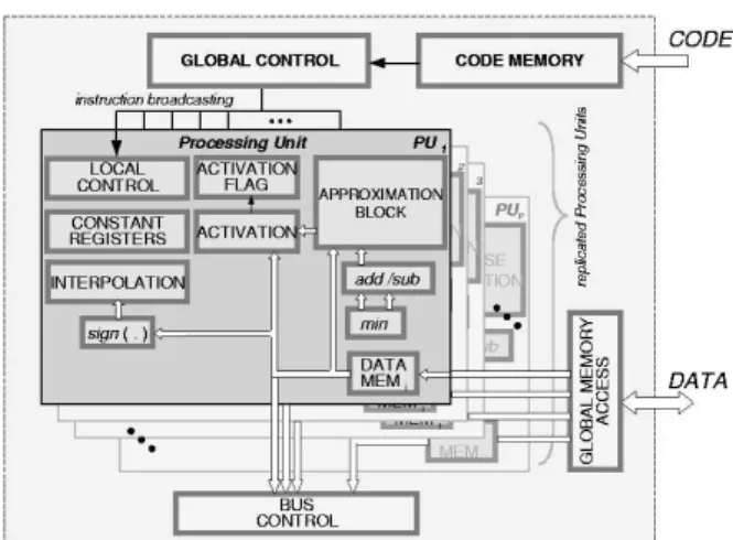
Fig. 3.Global architecture with replicated Processing Units (PUs).

PROCESSING UNIT

The Processing Unit (see Fig. 3) contains specific blocks implementing different stages of the algorithm: theINTERPOLATION BLOCKensures the initialization of the algorithm, and the APPROXIMATION BLOCK computes new pixel values. Each PU has a register containing the ACTIVATION FLAGs for its part of the

image. The activation flag is used as a mask controlling the PU activity. All the Processing Units, whose currently processed point is active (the activation flag is set) execute the instructions, otherwise they are idle, except of sending their values to the east- and west-side neighbors.

Note that the input data are stored in a non-shared data memory. Therefore, all the units can access to its data simultaneously at the given time. The memory is a double-port memory; before the execution of the algorithm, the data are uploaded by using a global access port (not given in the schematics) and read after. Recall that the Massive Marching uses the 4-neighborhood. In order to reduce the number of interconnections, we use bi-directional buses for the communication with the adjacent PUs. The bus direction is controlled by the signals t_east and t_west derived fromclk 2.

Neighborhood retrieval

The complete neighborhood of a point (cf. Fig. 4(b)) is obtained in two clock cycles in the following way (Fig. 4(a)). With a rising edge of the clock a newSOUTHvalue is read from the local data memory whereas the old valuesSOUTHandCENTERare shifted upwards (e.g. 112, 113, 114). The values EAST and WEST are read from the bus on the falling clock edges. First, the WEST value is read from the west-side adjacent PU while theSOUTHpoint value is being sent to the east-side adjacent PU. On the next falling edge is read theEASTpoint while theCENTERpoint is being sent to the west-side adjacent PU. The complete neighborhood is ready immediately after the reading of theEAST point (indicated by the dashed line). The same communication protocol also applies to filtering.

(a)

(b)

Note that the choice of the image division affects only the communication procedure between the adjacent processing units and not their internal architecture.

Approximation block

Instead of computing the exact value of Eq. (5), requiring computation of a square and square root, we propose to use an approximation. The approximation allows to preserve the necessary sub-pixel precision while reducing the implementation cost. Two types of approximations have been tested, the piecewise linearization and look-up-table (LUT). The functional scheme of the tested approximation blocks is given by Fig. 5. The Eq. (5) is rewritten in the form

u p

ux p)/ uy p

2 / gdiff

ux pc& uy p

(11)

which is, for the hardware implementation, approximated by either a linear approximation or a look-up-table

ˆ

uLinlApprox p

ux p)/ uy p

2 / ai

ux& uy

)/ bi

(12)

ˆ

uLUT p

ux p)/ uy p

2 / ai (13)

The number of operations to obtain ˆuLinlApprox p

reduces to three additions, one subtraction and two multiplications and for ˆuLUT p only two

additions and one multiplication (paid by higher memory requirements for comparable accuracy). The computation is done with a fixed-point precision. A comparative study of the implementation cost is presented below.

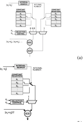
The implementation of the approximation is given by Fig. 5. The input signals are

ux & uy

and ux/

uy. (The terms ux and uy are obtained by two

comparators in the MIN block (Fig. 3)). The former enters also in the Interval Search block generating the address (interval number) of the register containing the corresponding approximation constants ai and bi (cf.

Fig. 6(a)). TheSELECTION CONTROLblock is testing whether the values ux, uy are finite. If both values

are finite (pixels have already been activated) then the distance is computed by using Eq. (11). If only one of the valuesux,uyis finite then the distance computation

reduces to addition of one to the finite value: the approximation constants are replaced in order to add 1 to the minimal neighbor. Recall that both values cannot be infinite in the same time since such a point would not be activated.

(a)

(b) Fig. 5. Internal block architecture of the Approximation Block; (a) Piecewise linearization, (b) Look-Up-Table.

Fig. 6.Interval Search and Activation Request block.

The computation process is completely pipelined. After an initial latency of 10 clock periods, the result is obtained in one clock period. The approximation block as it is given here can calculate the distance in one clock cycle only for"m 1. For"

V

1, the multiplier

must perform two additional multiplications. The overall bandwidth of the architecture will be lower unless two additional multipliers (or approximations) are used.

Pixel activation

Image Anal Stereol 2003;22:121-132

signals ARN, ARS, ARE, ARW - Activation Request to North, South, etc.). As soon as all the flags are inactive the algorithm ends.

EXPERIMENTAL RESULTS

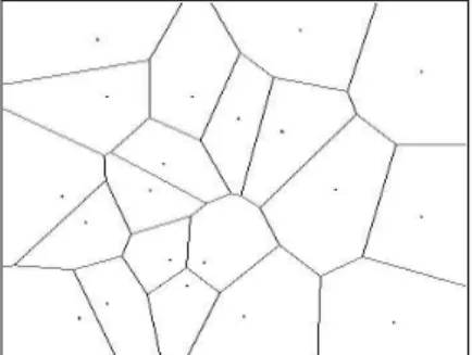
In order to prove the validity of the algorithm, we illustrate the behaviour of Massive Marching on computation of the Voronoï tesselation for a given set of points in a 2D euclidian space. In this case, we consider ", p 1 for n p po (see Fig. 7). Note

that if needed, the propagation of labels can be done simultaneously with the propagation of the distance.

(a) Exact, computed on Delaunay triangulation

(b) Massive Marching

(c) Fast Marching

Fig. 7. The Voronoï tessellation obtained by Massive Marching, compared to Fast Marching.

The result achieved by Massive Marching is compared to the exact result and to the result obtained by the sorted heap algorithm (Sethian, 1996). Slight differerence is due to i) an error of the Fast Marching induced by the direction of the scanning and ii) an approximation error of Massive Marching.

We have tested the accuracy of the result with respect to two factors: i) the approximation type of the Godunov numerical scheme and ii) the number of fractional bits of the fixed-point implementation of the approximation block. We have observed the error in q ∞ in the result with respect to the exact solution

simulated with “double” precision in C. Recall that the norm q ∞ corresponds to the maximum of the vector

elements. Here, it represents the upper bound of the error.

0 0.2 0.4 0.6 0.8 1 0.7

0.75 0.8 0.85 0.9 0.95 1

|u_x(p)−u_y(p)|

fdiff

(a) Original function of the Godunov scheme

0 0.2 0.4 0.6 0.8 1 0.7

0.75 0.8 0.85 0.9 0.95 1

|u_x(p)−u_y(p)|

fdiff

(b) Linear approximation with 4 intervals

0 0.2 0.4 0.6 0.8 1 0.7

0.75 0.8 0.85 0.9 0.95 1

|u_x(p)−u_y(p)|

fdiff

(c) Inequally spaced

LUT approximation

with 5 intervals

0 0.2 0.4 0.6 0.8 1 0.7

0.75 0.8 0.85 0.9 0.95 1

|u_x(p)−u_y(p)|

fdiff

(d) Inequally spaced

LUT approximation

with 15 intervals

0 0.2 0.4 0.6 0.8 1 0.7

0.75 0.8 0.85 0.9 0.95 1

|u_x(p)−u_y(p)|

fdiff

(e) Inequally spaced

LUT approximation

with 30 intervals

(a)

(b)

(c)

(d)

(e)

Fig. 9. Iso-distance lines obtained with various approximations (8+8 bits of precision); (a)

Original function of the Godunov scheme,

(b) Linear approximation with 4 intervals,

(c) LUT approximation with 5 intervals, (d) LUT approximation with 15 intervals, (e) LUT approximation with 30 intervals.

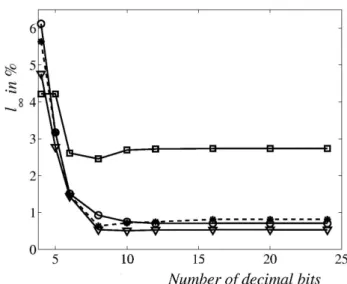
Fig. 10. Error (in q ∞) of the look-up-table

approximation compared to the exact solution depending on the fractional part width. Rectangles: LUT 5 intervals, circles: LUT 15 intervals, triangles: LUT 30 intervals; asterisks: piecewise linearization.

Two approximation types of the functiongdiffwere used: a piecewise linearization with four intervals

andlook-up-tableapproximation with five, fifteen and

thirty steps, see Fig. 8. The first and the last elements in the look-up-tables are exact (equal to 1kr 2 and 1) in

order to minimize the error in the left, right, up and down and diagonal directions. The other values are obtained as to distribute the error evenly over the entire interval 0

1. The distance results can be visually

assessed in Fig. 9 on the iso-distance lines given in the same figure for 8+8 bit precision. The test image contains three sources: a letter M, straight line and a point. The approximation error (inq ∞) with respect to

the exact result is given in Table 1.

Table 1. Error of approximation of the Godunov scheme given by Fig. 9.

Approx. type Linear. LUT LUT LUT

(interval no.) 4 5 15 30

Errorq ∞(%) 0.3 3.9 1.2 0.9

Image Anal Stereol 2003;22:121-132

Table 2.Overall (approximation plus rounding) error

inq ∞ of the result in Fig. 9(b, c, d and e) to the exact

result Fig. 9(a).

Approx. type Linear. LUT LUT LUT

(interval no.) 4 5 15 30

Error q ∞ 8 bits

(%) 0.64 2.45 0.92 0.54

Error q ∞ 16 bits

(%) 0.81 2.74 0.70 0.53

Simultaneously with the error introduced by the approximation and rounding error, see Fig. 10, we have observed the implementation cost in terms of the number of equivalent NAND gates in the netlist, reported by the compilator, before the optimization and routing on a specific chip (only for precision 8+8 and 8+16 bit integer+fractional part). For the surface estimation cf. Tables 3 and 4 below.

Table 3.Surface estimation of the approximation block 8+8 bits of precision (integer+fractional part).

Approx. type Piecewise lin. LUT LUT LUT

(interval no.) 4 5 15 30

Surface after optimization (NANDs) 10132 4031 6920 13856

Memory bits 128 80 240 480

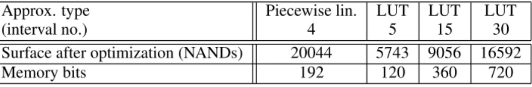
Table 4.Surface estimation of the approximation block 8+16 bits of precision (integer+fractional part).

Approx. type Piecewise lin. LUT LUT LUT

(interval no.) 4 5 15 30

Surface after optimization (NANDs) 20044 5743 9056 16592

Memory bits 192 120 360 720

Note that when using the piecewise linearization the surface requirements increase considerably (about twice of equivalent NANDs) if the accuracy increases from 8+8 to 8+16 bits (integer plus fractional part). On the other hand the surface occupation grows linearly when the look-up-table is used: increase by some 20% to 40% of equivalent NANDs and by one third of memory bits. The nonlinear increase of the implementation cost between the 8+8 and the 8+16 accuracy is due to the use of a highly optimized multiplier/accumulator.

CONCLUSIONS

This paper proposes a SIMD-type architecture for curve-evolution PDEs. This architecture has already been used for filtering by linear diffusion, see Gijbels

et al. (1994). In this paper is shown that the same

architecture type can also be used for the narrow-band like algorithms.

Obviously, the activity of Processing Units arranged in a linear array is unbalanced for narrow-band like algorithms. The activity distribution depends on the geometric form of the objects. This inconvenience is the price paid for the advantage

that without major modifications this architecture can run algorithms consisting of several stages, e.g. filtering followed by watershed or voronoï tessellation computation. The only modification consists in reconfiguration of the approximation blocks by uploading new values in the look-up-tables or the linear approximation registers. The algorithm is then executed by broadcasting corresponding high level instructions to the Processing Units.

For implementation on a FPGA, the maximum clock frequency we have obtained is 150MHz. One point is processed in two clock cycles (Jacobi plus Gauss-Seidel) which gives a theoretical bandwidth of one Processing Unit 75 10

6 _points

s

1_{. The worst} execution time estimation for the QCIF format (176 pixels wide by 144 high) with the distance source in a corner is 400µs.

We have observed that even if implemented sequentially in some situations (for denoised filtered images) the Massive Marching outperforms algorithms using ordered structures. For heavily noised input images, the Massive Marching performance remains comparable to other algorithms despite frequent reactivations.

Future work: Extension of Massive Marching

algorithms on big 3D images is penalized by excessive memory requirements of large, real-number-priority ordered structures. The use of Massive Marching may be advantageous because of the absence of any ordered waiting structures.

A better activity distribution would be achieved with processing units retrieving points waiting in a FIFO-like queue. Suppose a completely pipelined, random-access capable prefetch so that the neighborhood is retrieved in one clock cycle. The theoretical execution time will be t N

P cycles,

where Pis the number of pipelined processing units. The surface activity will be more balanced. An efficient neighborhood prefetch therefore needs to be found so that several pipelined processing units could be used.

REFERENCES

Boué M, Dupuis P (1999). Markov chain approximations for deterministic control problems with affine dynamics and quadratic cost in the control. SIAM J Numer Anal 36:667–95.

Danielsson P (1980). Euclidean distance mapping. Comput Vision Graph 14:227–48.

Dejnožková E (2002). Massive marching : A parallel computation of distance function for PDE-based applications. Tech. Rep. N-17/02/MM, ENSMP, Center of Mathematical Morphology.

Dejnožková E, Dokládal P (2003a). A multiprocessor architecture for PDE-based applications. Visual Information Engineering, VIE 2003. Proceedings. Dejnožková E, Dokládal P (2003b). A parallel

algorithm for solving eikonal equation. In: IEEE International Conference on Acoustics, Speech and Signal Processing, ICASSP. Proceedings.

Eggers H (1997). Fast parallel euclidian distance transformation inZn_{. SPIE Proceedings 3168:33–40.}

Gijbels T, Six P, Gool LV, Catthoor F, Man HD, Oosterlinck A (1994). A VLSI architecture for parallel non-linear diffusion with applications in vision. IEEE Workshop on VLSI Signal Processing .

Gomez J, Faugeras O (1992). Reconciling distance functions and level sets. Tech Rep No: 3666, INRIA. Kimmel R (1995). Curve Evolution on Surfaces. Ph.D.

thesis, Technion Israel Institute of Technology.

Kimmel R, Sethian JA (2001). Optimal algorithm for shape from shading and path planning. J Math Imaging Vis 14:237–44.

Meyer F, Maragos P (1999). Multiscale morphological segmentations based on watershed, flooding, and eikonal PDE. In: Nielsen M, Johansen P, Olsen O, Weickert J, eds., Scale-Space Theories in Computer Vision, no. 1682 in Lecture Notes in Computer Science. Springer-Verlag, 351–62.

Osher S, Sethian J (1988). Fronts propagating with curvature-dependent speed: Algorithms based on Hamilton-Jacobi formulations. J Comput Phys 79:12– 49.

Osher S, Shu CW (1991). High-order Essentially Non-oscillatory schemes for Hamilton-Jacobi equations. SIAM J Numer Anal 28:907–22.

Paragios N (2000). Geodesic Active Regions and Level Set Methods : Contributions and Applications in Artificial Vision. Ph.D. thesis, Université de Sophia Antipolis. Perona P, Malik J (1988). A network for multiscale

segmentation. Proceedings IEEE International Symposium Circuits and Systems CISCAC88 :2565–8. Rumpf M, Strzodka R (2001). Level set segmentation in

graphics hardware. In: Proceedings ICIP 2001. Sapiro G (2000). Geometric Partial Differential Equations

and Image Analysis. Cambridge: Cambridge University Press.

Sethian JA (1996). Level Set Methods. Cambridge: Cambridge University Press.

Sethian JA (1999). Fast marching methods. SIAM Review 41:199–235.

Siddiqi K, Kimia B, Shu CW (1997). Geometric shock-capturing ENO schemes for subpixel interpolation, computation and curve evolution. Graph Model Im Proc 59:278–301.

Suri J, Singh S, Reden L (2002). Computer vision and pattern recognition techniques for 2-D and 3-D MR cerebral cortical segmentation: A state-of-the-art review. Int J Patt Anal Ap 5:46–76.

Tsai Y (2000). Rapid and accurate computation of the distance function using grids. Tech. Rep. 17, Department of Mathematics, University of California, Los Angeles.

Verbeek P, Verwer B (1990). Shading from shape, the eikonal equation solved by grayweighted distance transform. Patt Recogn Lett 11:681–90.

Weickert J, ter Haar Romeny BM, Viergver MA (1998). Efficient and reliable schemes for nonlinear diffusion filtering. In: IEEE Trans Image Proc, vol. 7. 398–410. Zhao H, Chan T, Merriman B, Osher S (1996). A variational