On intervened negative binomial distribution and some of its properties

ON INTERVENED NEGATIVE BINOMIAL DISTRIBUTION AND SOME OF ITS PROPERTIES

C. Satheesh Kumar, S. Sreejakumari

1. INTRODUCTION

Since 1985, intervened type distributions have received much attention in the literature. These types of distributions provide information on the effectiveness of various preventive actions taken in several areas of scientific research. (Shan-mugam, 1985) introduced an intervened Poisson distribution (IPD) as a replace-ment for positive Poisson distribution where some intervention process changes the mean of rare events. The IPD has been further studied by (Shanmugam, 1992), (Huang and Fung, 1989) and (Dhanavanthan, 1998, 2000). (Scollnik, 2006) developed the intervened generalized Poisson distribution and (Kumar and Shibu, 2011) considered amodified version of IPD. (Bartolucci et al., 2001) stud-ied an intervened version of geometric distribution with following probability mass function (p.m.f.).

1

2 1

1

(1 )(1 ) 1

1

( )

(1 ) 1 ,

x x

x

x

p P X x

x



   



  





 _

  

 _

  _{ }

 _{ }



(1)

in which x1, 2,3, ..., 0  1 and  0.

Through this paper we develop an intervened version of negative binomial dis-tribution, which we called as intervened negative binomial distribution (INBD). Negative binomial distribution have found applications in several areas of re-search such as accidental statistics, birth and death process, medical sciences, psy-chology etc. For details see (Johnson et al., 2005). In most of these fields there are situations in which observations commence only when at least one event occurs due to some intervention. For this reason a distribution with support {1, 2,3, ...} is quite relevant and hence we develop a distribution which is suitable for ac-commodating such intervention mechanisms.

factorial moments. We also obtain a recurrence relation for probabilities of INBD in section 2. In section 3 we consider the estimation of parameters of INBD by various methods of estimation such as method of factorial moments, method of mixed moments and method of maximum likelihood. A real life data is consid-ered for illustrating these procedures.

2. INTERVENED NEGATIVE BINOMIAL DISTRIBUTION

Let Y be a random variable having zero truncated negative binomial distribu-tion with following p.m.f., in which 0  1, r > 0 and y = 1,2,3,... .

1

( ; , ) ( ) (1 )

1

r y

y r

p y r P Y y

r

    _   _   

  , (2)

where _{   [1 (1 ) ] .}r 1 _{The characteristic function of Y is} ( ) (1 ) [(1r it) r 1]

Y t e

 _ _ _  _{ (3)}

Let Z be a random variable following negative binomial distribution with p.m.f.

1

( ; , , ) ( ) (1 ) ( ) ,

1

r z

z r

f z r P Z z

r

    _   _   

  (4)

in which z = 0,1,2,...,  > 0, r > 0 and  0 such that 01. The characteristic function of Z is

( ) (1 ) (1r it) .r

Z t e

 _{ } _  ₍₅₎

Assume that Y and Z are statistically independent. Define X = Y + Z. Then the characteristic function of X is

( ) ( ). ( )

X t Y t Z t

  

_( , , ) ((1_{  r e}it)r _1) (1_eit) .r ₍₆₎

where

( , , )_{  r }[(1 _) (1 _)]r

   

( ) ( , , )[(1 ) r 1](1 ) r

X

P s _   r _s  _{ }s  ₍₇₎

Clearly P_X(1) 1 .

Result 2.1Let X follows INBD with p.g.f. (7). Then the probability mass function gx= P(X=x) of INBD is the following, for x1, 2,3, ..., in which 0< θ <1 and

 >0.

1 2

0 ( , , )

( ) ( )

! [ ( )]

x x

y x

y

x r

g x y r y r

y x

r

    _

 

 



 

 _{ }   

 



Proof From (7) we have the following:

0

( ) x

X x

x

P s g s









₂ 1

0 0

( , ) ( )

( ) ( )

! [ ( )]

x x

y

x y

x s

x y r y r

y x

r

  



 

 



 



 

 _{ }   

 





On equating coefficient of sx _{on right hand side expression of (9) and (10), we} get (8).

Remark 2.1When r =1, (8) reduces to the p.m.f. of intervened geometric distribu-tion as given in (1).

Result 2.2For any positive integerk,the kth _{factorial moment}  k

 of INBD is

  1 2 2

( ) (1 ) ( )

( ) [ ( )]

k k

k

k r k

r r

  

  

 

 

  (11)

in which 1

1 (1 )

 _ _  _, 1

2 (1 )

 _ _  _{and for k1,}

2

0 1

( ) [ ( )][ ( )] .

y k

y

y

k k y r y r

k

 



   _{ }     _ _

   



  0

( ) ( )

X k

k

H t   t









P_X(1 )t

_( , , )([1 (1_{  r  t}) ]_ r _1)[1 (1_{ t})_]r

(11t) (1r 2t)r  (1 ) (12t)r

2 1

0 0 1

2 0

1 1

( )

1

(1 ) ( ) .

y k

k

k y

k k

k y r y r

t

k y y

k r

t k



 



 



 





 _{          } 

 

 _{     }



       

 

 

 

  _{ }

 

 



(13)

On equating coefficient of (k!) t on the right hand side expressions of (12) -1 k and (13), we get (11).

Remark 2.2 Putting k=1, 2, 3 in (11) we get the first three factorial moments of INBD as given below.

 

 

 

2 1

1

2 2 2

2 1 1 2

2

3 3 2

2 1 1 2 1 2

3

( 1) [ ( 1) 2 ]

( 1) ( 2) [ ( 1) ( 2) 3 ( 1) ( )]

r r

r r r r r

r r r r r r r r

   

     

       

  

     

         

(14)

Result 2.3 The mean E(X) and variance V(X) of INBD with p.g.f. (7) are the fol-lowing:

2 1

( )

E X r r (15)

and

2

2 2 1 1 1

( ) (1 ) (1 ) (1 ) ( )

V X r  r    r (16)

Proof follows from (14) in the light of the relation

2

( ) ( ( 1) ( ) [ ( )]

V X E X X E X  E X

_{     } 2 2 1 [ 1 ]   

  

Remark 2.3 When r =1 in (15) and (16) we get the E(X) and V(X) of intervened geometric distribution as

2 1

( )

E X    and

2

2 2 1 1 1

( ) (1 ) (1 ) (1 )

V X         .

Result 2.4INBD is over-dispersed or under-dispersed according as

2 2 2

2 (r 1) 1 r( 1)

        or 2 2 2

2 (r 1) 1 r( 1)         Prooffollows from Result 2.3.

Result 2.5The following is a simple recurrence relation for probabilities of INBD, for x ≥1.

1 1

1 0

( 1) x k (1 k ) ( ; , , ),

x x k

k

x g r     g  x   r

 



 



in which

1 0

( , ) ( )

( ; , , ) .

( 1) ( 1)

x

x x k

k

x k r

x r

r x k

 

   

  



 

 

  





Proof From (10) we have

0

( ) x

X x

x

P s  s g







₂ 1

0 0

( , ) ( )

( ) ( )

! [ ( )]

x x

y

x y

x s

x y r y r

y x

r

     _

 



 



 

 _{ }   

 





'

1 1

( ) ( 1) x

X x

x

P s x g s



 





( ) ( , ) (1 )

1 1 (1 )

r X

s

rP s r

s s s



 

  

  

 

    

 _{ }_{ }

    

 

 

0 0 0 0

( )k x k ( )k x k

x x

x k x k

r    s  g r    s  g

   



 

 

0 0

1

( , ) x( )x k

x x k

x r

r s g

x

       

 

    

 _{ }

 



1 1

0 0

(1 )

x

k k x

x k x k

r      g s



 





0 0

1

( , ) x ( )x x k

x k

x k r

r s

x k

      

 

     

 _{ }



 



1 1

0 0

(1 ) [ ; , , ]

x

k k x

x k

x k

r   g x   r s



 



 

 

 _   _

 

 

Now on equating coefficients of sx _{on the right hand side expressions of (20)} and (21), we get (17).

3. ESTIMATION

Here we discuss the estimation of parameters of the INBD by method of fac-torial moments, method of mixed moments and the method of maximum likeli-hood.

Method of factorial moment

In method of factorial moments, the first three factorial moments of the INBD are equated to the corresponding sample factorial momentsm1, m2 and m3 and thus we obtain the following system of equations:

2 1 1

r r m (22)

2 2 2

2 1 1 2 2

( 1) ( 1) 2

r r  r r   r   m (23)

3 3 2

2 1 1 2 1 2 3

( 1)( 2) ( 1)( 2) 3 ( 1) ( )

r r  r  r r r   r r     m (24)

where 1 and 2 are given in (11). Now, the parameters of the INBD are esti-mated by solving the non-linear equations (22), (23) and (24) using MATHCAD.

Method of mixed moments

In method of mixed moments, the parameters are estimated by using the first two sample factorial moments and the first observed frequency of the distribu-tion. That is, the parameters are estimated by solving the following equation to-gether with (22) and (23).

1

[(1 ) (1 )]r_r p ,

N

  

   (25)

where p1 is the observed frequency of the distribution corresponding to the ob-servation x=1 and N is the total observed frequency.

Method of maximum likelihood

Let a(x) be the observed frequency of x events, y be the highest value of x ob-served. Then the likelihood of the sample is

( ) 1

[ ( )]

y

a x x

L g x







which implies

log L = 1

( ).log[ ( )]

y

x

a x g x





Assume that the parameter r of INBD is known. Let ˆ and ˆ denotes the maximum likelihood estimates of  and  respectively. Now, ˆ and ˆ are ob-tained by solving the normal equation (26) and (27) given below.

log 0 L 



  implies

_{2 1}

1 1

( ) ( ) [ ] 0

y y

x x

x a x r a x  

 

  

log 0 L 



  implies

1

( ). ( , ) 0

y

x

a x D  







in which

1

1 0

1

0

. ( ). ( ). .

( , )

1

( ). ( )

x

y y

x

y y

x

x y r y r y

y _r

D

x

x y r y r

y



  

 



 





 

 

   

  

   

 

 

 

_{   }



  _{ }

  

 _{ } 

 _{ } 

 





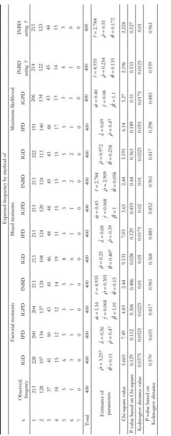
Here estimator of r is used for obtaining the maximum likelihood estimates ˆ and ˆ of  and  respectively. Let r denotes the factorial moment estimator of r and r denotes the mixed moment estimate of r. Table 1 gives the data re-lated to the distribution of number of articles of theoretical statistics and prob-ability for years 1940-49 and initial letters N-R of the author’s name, for details, see (Kendall, 1961). Here we present the fitting of intervened geometric distribu-tion (IGD), intervened Poisson distribudistribu-tions (IPD), intervened generalized Pois-son distributions (IGPD) and intervened negative binomial distributions (INBD). From Table 1, it is obvious that INBD is more suitable for the data compared to IGD, IPD and IGPD.

ACKNOWLEDGMENTS

The authors would like to express their sincere thanks to the Editor and the anonymous Referee for carefully reading the paper and for valuable suggestions.

Department of Statistics C. SATHEESH KUMAR

University of Kerala, Kariavattom, Trivandrum, India

Department of Statistics S. SREEJAKUMARI

TABLE 1

Distribution of number of articles of

theo

retical sta

tistics and

probability for ye

ars

from 1940-49 and i

nitial letters N-R of

th e au th or ’s name Exp ect ed f reque ncy by meth od of Fa ct oria l moment s M ix ed moments M ax imum likelihood x Ob se rv ed . freqe ncy IGD IPD IGPD INBD IGD IPD IGPD INBD IGD IPD IGPD

INBD _usin

g

r



INBD _using

r

1

213

228 200 204 213 213 213 213

213 222 191 206 214 215 2 128

107 134 137 124 108 124 120

124 113 140 134 122 123 3 37 41

50 43 45 46 48 48

45 43 48 43 45 44 4 18 15

12 12 14 19 11 15

13 15 17 13 14 15 5 3

6 3 3 3 8 3 3

3 5 3 3 4 3 6 1

3 1 1 1 6 1 1

2 2 1 1 1 0 7 0

0 0 0 0 0 0 0

0 0 0 0 0 0 Tota l 400

400 400 400 400 400 400 400

400 400 400 400 400 400 Estim ate s of par amet ers ˆ 3.25 7 ˆ 0.1 1     ˆ 0. 56 ˆ 0. 47     ˆ 1.16 ˆ 0.068 ˆ 1.01       4. 93 5 ˆ 0.30 1 ˆ 0.1 3

r  

    ˆ 0.2 5 ˆ 0. 407     ˆ 0. 68 ˆ 0.39     ˆ 0. 43 ˆ 0.068 ˆ 1       2.78 4 ˆ 2.90 9 ˆ 0.0 58

r  

    ˆ 0. 97 2 ˆ 0.2 58     ˆ 0. 69 ˆ 0.47     ˆ 0. 40 ˆ 0.0 8 ˆ 1.1       4. 93 5 ˆ 0. 25 4 ˆ 0.1 35

r  

    2.784 ˆ 0. 51 ˆ 0.172

r  

REFERENCES

A. A. BARTOLUCCI, R. SHANMUGAM, K. P. SINGH (2001), Developments of the generalized geometric

model with application to cardiovascular studies, “System Analysis Modeling Simulation”, 41, pp. 339-349.

P. DHANAVANTHAN (1998), Compound intervened Poisson distribution, “Biometrical Journal”, 40,

pp. 641-646.

P. DHANAVANTHAN (2000), Estimation of the parameters of compound intervened Poisson distribution,

“Biometrical Journal”, 42, pp. 315-320.

M. HUANG, K.Y. FUNG (1989), Intervened truncated Poisson distribution, “Sankhya”, Series B, 51,

pp. 302-310.

N. L. JOHNSON, A.W. KEMP, S. KOTZ (2005), Univariate Discrete Distributions, John Wiley and

Sons, New York.

M.G. KENDAL (1961), Natural law in Science, “Journal of Royal Statistical Society”, Series. A,

124, pp. 1-18.

C.S. KUMAR, D.S. SHIBU (2011), Modified intervened Poisson distribution, “Statistica”, 71, pp.

489-499.

D.P.M. SCOLLNIK (2006), On the intervened generalized Poisson distribution, “Communication in

Statistics-Theory and Methods”, 35, pp. 953-963.

R. SHANMUGAM (1985), An intervened Poisson distribution and its medical application, “Biometrics”,

41, pp. 1025-1029.

R. SHANMUGAM (1992), An inferential procedure for the Poisson intervention parameter,

“Biomet-rics”, 48, pp. 559-565.

SUMMARY

On intervened negative binomial distribution and some of its properties