Sharif University of Technology
Scientia IranicaTransactions A: Civil Engineering http://scientiairanica.sharif.edu
A comparison among data mining algorithms for outlier
detection using ow pattern experiments
M. Vaghe
a;, K. Mahmoodi
b, and M. Akbari
a a. Faculty of Civil Engineering, Persian Gulf University, Bushehr, Iran.b. Faculty of Marine Engineering, Amirkabir University of Technology, Tehran, Iran. Received 17 January 2016; received in revised form 15 May 2016; accepted 29 October 2016
KEYWORDS Outlier detection; Data mining; Flow pattern; Sharp bend channel; Vectrino.
Abstract.Accurate outlier detection is an important matter to consider prior to applying data to predict ow patterns. Identifying these outliers and reducing their impact on measurements could be eective in presenting an authentic ow pattern. This paper aims to detect outliers in ow pattern experiments along a 180-degree sharp bend channel with and without a T-shaped spur dike. Velocity components have been collected using 3D velocimeter called Vectrino in order to determine the ow pattern. Some of outlier detection methods were employed in the paper, such as Z-score test, sum of sine curve tting, Mahalanobis distance, hierarchical clustering, LSC-mine, self-organizing map, fuzzy C-means clustering, and voting. Considering the experiments carried out, the methods were ecient in outlier detection; however, the voting method appeared to be the most ecient one. Briey, this paper calculated dierent hydraulic parameters in the sharp bend and made a comparison between them for the sake of studying how eective running the voting method is in mean and turbulent ow pattern variations. The results indicated that developing the voting method in the ow pattern experiment in the bend would cause a decrease in Reynolds shear stress by 36%, while the mean velocities were not signicantly inuenced by the method.
© 2018 Sharif University of Technology. All rights reserved.
1. Introduction
A true understanding of the ow pattern further improves the recognition of ow characteristics and the parameters eective in it. It is of high importance and results in creating optimum designs in the case of hydraulic structures such as spur dikes, preventing huge compensation and fatality. Spur dikes are hy-draulic structures constructed to protect canals and rivers against scour and erosion [1]. Whenever a spur
*. Corresponding author. Tel.: +98 77 31222401; Fax: +98 77 33440376
E-mail addresses: [email protected] (M. Vaghe); [email protected] (K. Mahmoodi); [email protected] (M. Akbari)
doi: 10.24200/sci.2017.4182
dike is located in the outer bank of a bend, the scour process becomes a complex phenomenon. The ow eld at a spur dike is coupled with a complex 3D separation of approach ow upstream and a periodic vortex shedding downstream of the spur dike [2,3].
The experimental data are considered as prelim-inary data for further numerical analyses and math-ematical modeling; therefore, they need to be error-free. In practice, measuring error-free data is nearly impossible, and some data inconsistent with the normal pattern of the statistical population arise for dierent reasons. Data collection for ow pattern determination is no exception and may encounter inaccuracies and inconsistencies as well. Such data play a pivotal role in predicting ow patterns. As they might have arisen due to an error in measurement, detecting and eliminating them from the collected values are the
requirements which help obtain high-reliability data; then, the results obtained from the data analysis would be perfect and reliable. An outlier can indicate any errors in data that may arise due to the natural behav-ior of the ow under unique circumstances. Therefore, detecting them can provide highly useful information on the nature of the ow unknown so far. Accordingly, detecting outlier, while collecting required data to determine ow pattern, is considered an inevitable necessity.
Outlier detection is a primary step in many data mining applications. Outlier detection has been used for centuries to detect and, where appropriate, remove anomalous observations from data. There are some factors involved in the existence of outliers consisting of mechanical faults, changes in system behavior, fraudulent behavior, human mistake, instrument error or simply through natural deviations in populations [4]. Goring and Nikora [5] suggested a new method for detecting spikes in acoustic Doppler velocimeter data sequences. The new method was shown to have supe-rior performance compared to various other methods, along with the added advantage that it required no parameters. Of the methods considered, the phase-space thresholding method is the most suitable one for detecting spikes in the data related to a down-looking ADV. They concluded that for ADV data with sampling frequencies from 25 to 100 Hz, the best solution is to use 12 points on either side of the spike to t a third-order polynomial that was interpolated across the spike. Mori et al. [6] examined the ADV velocity measurements in bubbly ows. They applied the despiking algorithm based on the 3D phase space method and discussed bubble eects on ADV velocity. The results showed that there is no clear relation-ship between velocity and ADV's correlation/Signal-to-Noise Ratio (SNR) in bubbly ow. Moreover, spike noise ltering methods based on low correlation and signal-to-noise ratio were not adequate for bubbly ow, and the true 3D phase space method signicantly removed spike noise of ADV velocity in comparison with the original 3D phase space method. Duncan et al. [7] developed a new method of outlier detection for both PTV and PIV data based on the original algorithm of Westerweel and Scarano [8]. The current method takes two to three times as long as the universal outlier detection method of Westerweel and Scarano (2005), which is mainly due to the time taken by the tessellation process. The changes included a dierent denition of neighbors based on Delaunay tessellation, weighting of neighbor velocities based on the distance from the point in question, and an adaptive tolerance to account for the dierent distances to neighbors. The new algorithm worked equally well for PIV and PTV up to a level of spurious data of about 15%, far higher than should be encountered with good experimental
techniques. Razaz and Kawanisi [9] presented several dierent techniques for detecting and replacing multi-point spikes in the acoustic Doppler sensor data time series. Among the methods considered, the modied wavelet method was conrmed to be the most suitable approach for detecting spikes. To improve the per-formance of the wavelet method, cutos, consisting of the universal threshold and a robust measure of scale, were employed. The developed methods for replacing identied spikes combine times series analyses with a straightforward method, i.e. polynomial interpolation, to generate substitutions retaining both the trends and uctuations in the surrounding clean data. The results indicated that the methodology was capable of restoring the contaminated signal in such a way that its statistical and physical properties correlate well with those of the original record.
This study mainly aims to detect outliers in ow pattern data collected via Vecterino velocimeter using various outlier detection methods and, consequently, to suggest solutions for identifying such data in a sharp bend. A variety of denitions have been proposed for outliers so far, although none of them have been comprehensive and they have been only described rather than dened; actually, providing a denition of outliers depends on the type of data and their use. In this paper, outliers are considered as the data not consistent with the normal pattern of the total data, and they signicantly dier from other observations in a way that they appear to be generated with a dierent mechanism [10].
Researchers have categorized outlier detection methods in dierent categories. In this paper, they are classied in four groups as follows:
1. Statistical methods [11]: These approaches are based on specic distribution of observations, or statistical estimations of distribution of unknown parameters, mostly with high-dimensional data, and when there is no information available on distribution of data, these methods are useless;
2. Distance-based methods [12]: These methods detect outliers by calculating the distance between the points by means of a distance metric function such as Euclidian function;
3. Cluster-based methods [13]: In these methods, the data are rst classied in clusters due to homo-geneity. If data do not belong to any clusters, or the cluster is considerably smaller than the others are, it seems to be an outlier candidate;
4. Density-based methods [14]: These methods have proven to be very eective in determining the density of the nearest neighbors in order to detect outliers.
least one outlier detection method is selected from each of the categories mentioned above to be employed un-der two conditions: with a T-shaped spur dike located in the bend and without spur dike. Therefore, Z-score test, sum of sine curve tting, Mahalanobis distance, hierarchical clustering, LSC-mine, self-organizing map, fuzzy C-means clustering, and voting are the methods employed in this study. In the following, these methods and characteristics of the case study will be introduced, and the factors or mechanisms causing outliers during the experiments together with the obtained results are discussed in the paper. Eventually, dierent hydraulic parameters in mean and turbulent ows after eliminating the detected outliers will be compared.
2. Methodologies
This section presents the experimental setup, dataset under investigation, and methods.
2.1. Experimental setup and procedure 2.1.1. Laboratory ume and spur dike
In this research, a bend ume with a central angle of 180 degrees, width of 1 m, and height of 0.7 m, glass sidewalls, and steel frames was designed and built in a hydraulic laboratory of Persian Gulf University of Bushehr, Iran. A plan view of the ume and its geometry is presented in Figure 1. As displayed, the ume consists of a 6.5 m long upstream straight reach and a 5.1 m long downstream straight reach. As seen in Figure 1, these two straight reaches are connected to each other by means of a 180 degree bend having external curvature radius of 2.5 m. Considering 1m width of the channel (B) and 2 m central radius of the bend (R), based on Leschziner and Rodi classica-tion [15], the ume has a sharp bend. The bed is rigid and the material with average diameter of 0.001 m is used to provide the desired bed roughness. To supply the required water in the channel, storages with the capacity of 30 m3 and a pump of 0.095 m3/s delivery
capacity are used. It is worth mentioning that the ow depth is of 0.2 m at the start of the bend, and it is
Figure 1. The schematic plan view of the laboratory ume and its geometry.
controlled using an adjustable buttery gate located at the downstream end of track during experiments. Therefore, Froude and Reynolds numbers are constant and equal to 0.34 and 119000, correspondingly [16].
As seen in Figure 1, the spur dike is T-shaped in the plan and installed at the outer wall at a 90-degree angle of the bend. The spur dike wing and web are 0.15 m long while their thickness and height are 0.01 m and 0.4 m, respectively. The spur dike used in laboratory is made of Plexiglas with semi-circle corners wing.
2.1.2. Velocimeter
In order to measure velocity components and model ow pattern, a three-dimensional velocimeter called Vectrino is used. This instrument is a new genera-tion of ADV series and is considered as one of the most advanced instruments known due to its high accuracy and the ability of recording three-dimensional velocities. Depending upon conguration of sensors, they are called either side-looking or down-looking probes connected to a computer by means of special cables, on which instrument software is installed. By connecting the instrument to computer, les can be managed simply and velocity monitoring is displayed using a software product installed on the computer. Data recorded by Vectrino are adjustable in a range of 0:01 to 7 m/s and the accuracy equals 0:5% of data (1 mm/s) [17]. In this study, to carry out experiments, frequency and time are assumed 25 HZ and 1 min, respectively; hence, the instrument is able to record at most 1500 data of velocity in three directions (U: velocity component in X-direction, V : velocity component in Y-direction, and W : velocity component in W-direction). In Figure 2, arrangement of Vectrino and its sensors on the channel are presented.
2.1.3. Mesh grids and study area
During the process of carrying out experiments to predict and present ow pattern, a ner mesh is applied around and downstream of spur dike, compared to a bend without spur dike. Overall, the 3D ow velocity prole has been measured at 36 cross-sections, 22 lon-gitudinal sections, and 5 depth levels. In this research,
Figure 2. Location of Vectrino and sensors over the open channel.
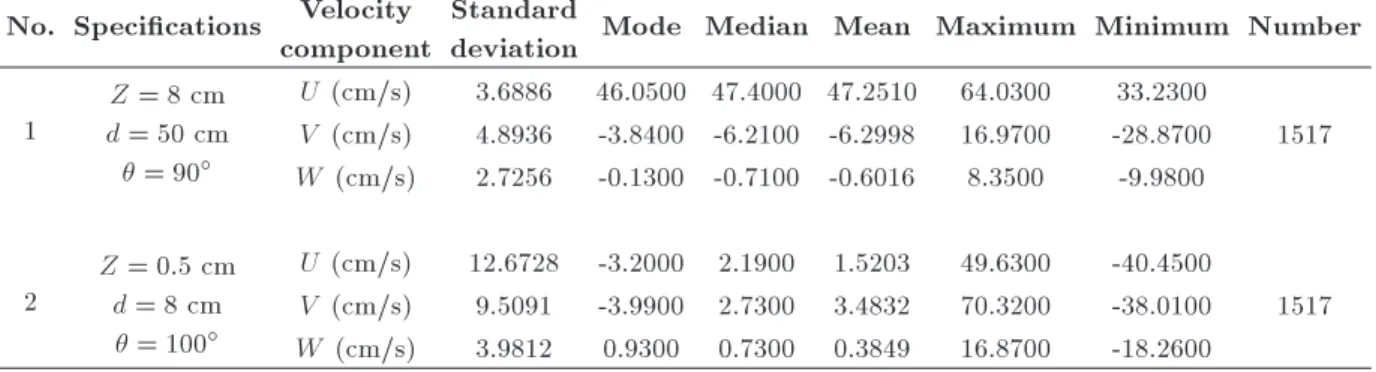
Table 1. Details of the data points. No. Specications Velocity
component
Standard
deviation Mode Median Mean Maximum Minimum Number 1
Z = 8 cm d = 50 cm = 90
U (cm/s) 3.6886 46.0500 47.4000 47.2510 64.0300 33.2300
V (cm/s) 4.8936 -3.8400 -6.2100 -6.2998 16.9700 -28.8700 1517 W (cm/s) 2.7256 -0.1300 -0.7100 -0.6016 8.3500 -9.9800
2
Z = 0:5 cm d = 8 cm
= 100
U (cm/s) 12.6728 -3.2000 2.1900 1.5203 49.6300 -40.4500
V (cm/s) 9.5091 -3.9900 2.7300 3.4832 70.3200 -38.0100 1517 W (cm/s) 3.9812 0.9300 0.7300 0.3849 16.8700 -18.2600
Figure 3. 3D velocity distributions of the investigated points (U, V, and W).
the performance of the outlier detection methods has been shown in a case study on the coordinate of two points (velocity values in U, V, and W directions) of the recorded points. One of these points has been recorded in the presence of the T-shaped spur dike along a sharp bend, whereas the other one has been without it. The details of the investigated samples are shown in Table 1, and their diagram is depicted in Figure 3.
In the second column of Table 1 (on the left side), Z represents distance from the channel bed; is the horizontal angle; d is dened as the distance from the outer wall of the bend.
2.2. Statistical methods 2.2.1. Z-score test
Z-score test is a statistical test commonly used for detecting outliers in univariate data sets. Outliers are detected using the arithmetic mean and standard devi-ation; hence, its eect depends on sample members [18]. The derived equations are described as follows (Eqs. (1) and (2)):
Zscore(i) =xiSDx; (1)
where: SD =
1 n 1
Xn
i=1(xi x)
21=2: (2)
According to a general rule, Zscore(i) values, whose
ab-solute values exceed 3, are candidate outliers. However, such a threshold limit value has problems in itself [18]. Moreover, the maximum absolute value of Zscore (i) is
dened as (n 1)=pn, and none of the outlier data's Zscore (i) might exceed it. In the case of small data
set, it is more obvious. Totally, selecting the threshold limit value is generally related to the dataset and the decision-maker's considerations. The threshold limit value for datasets is assumed 3.5 in this research. 2.2.2. Sum of sines curve tting
The curve tting of the data is one of outlier detection methods and can be used in both univariate and mul-tivariate datasets. In order to detect outliers through this method, the residuals (the dierence between the real and estimated values) are rst calculated and then the greater values are selected as a candidate outlier. There are a variety of methods for curve tting. In this research, the sum of sines model ts periodic function to a series of data points (Eq. (3)):
y =Xn
i=1aisin(bix + ci): (3)
Here, ai is the amplitude; bi is the frequency; ci is the
phase constant for each sine wave term. In addition, n is dened as the number of terms in the series. To calculate these parameters, Trust-Region [19] and
Levenberg-Marquardt [20] are used. The threshold value for the datasets is 3.5 in this research. Moreover, there are 5 terms in the series.
2.2.3. Mahalanobis distance
The Mahalanobis distance is a known parametric mea-sure that relies on the estimate of the multivariate parameters distribution and the data covariance [21]. The covariance matrix is dened as follows (Eq. (4)):
Cov =n 11 Xn
i=1(xi x)(xi x)
T: (4)
Thus, the Mahalanobis distance can be computed by the following relation (Eq. (5)):
Mi=
q
(xi x)TCov 1(xi x): (5)
In this way, xi can be an outlier candidate if the
calculated value of Mifor xisample under investigation
is greater than the threshold limit value of t. In order to apply the Mahalanobis distance method in this paper, as in two methods previously addressed, the threshold value is dened 3.5. In fact, for the cases in which the Mahalanobis distance exceeds 3.5, that sample is considered as an outlier.
2.2.4. Hierarchical clustering
The goal of clustering is to identify a structure in an unlabeled dataset by objectively organizing data into homogeneous groups where the within-group-object similarity is minimized and the between-group-object dissimilarity is maximized [22]. In clustering through hierarchical methods, the clusters are determined hier-archically in a descending or ascending order of size. In this method, the nal clusters are given hierarchical order, normally like a tree, based on their generaliz-ability. The tree is called a Dendrogram. In this research, the single-link divisive clustering algorithm [23] is employed. It is one of the oldest and simplest clustering methods, known as the nearest neighbor method. The following measure is used to calculate how similar c1 and c2clusters are (Eq. (6)):
dc1;c2= mini2c1;j2c2(di;j); (6)
where i is a sample from c1cluster and j from c2cluster.
Since the hierarchical clustering methods provide both more detailed and accurate information, they seem to be suitable for analysis in detail. However, they are highly complicated and not appropriate in terms of calculation for larger data sets. One way to evaluate the quality of the formed cluster tree in reecting the data is to compare the cophenetic distance with the main distance between the data. If the clustering is valid, there is a strong correlation between the data link in the cluster tree and the data distance in the
distance vector. The cophenetic correlation coecient can be used to compare these two distances. The closer calculated coecient is to 1, the better reector cluster tree will be. The cophenetic correlation coecient can be calculated thorough Eq. (7) [24]:
c = P
i<j(Yij y)(Zij z)
P
i<j(Yij y)2Pi<j(Zij z)2; (7)
where Yij represents the main distance between i and
j points in Y direction; Zij is cophenetic distance
between i and j in Z direction; y and z are averages of the values of Y and Z data groups, respectively.
In this research, to apply the hierarchical clus-tering method to the datasets, with regard to the conducted experiments and after trial and error, the values of two parameters of k (the number of clusters) and t (threshold) are assumed as 5 and 30, correspond-ingly. Euclidean function is selected for measuring the distance between data points.
2.2.5. LSC-mine
LSC-mine [25] is a density-based outlier detection method in multivariate data sets. In the pursuit of implying LSC-mine method, the following steps must be taken:
Calculating k-distance of p;
Finding k-distance neighborhood of p (Nk(p));
Calculating local sparsity ratio of object p (lsrk(p));
Calculating the pruning factor;
Calculating the local sparsity coecient of p (LSCk(p)).
The local sparsity coecient of k is dened as the proportion of the mean of local sparsity ratio of p to k-nearest neighbors (Eq. (8)):
LSCk(p) =
P
o2Nk(p)
lsrk(o)
lsrk(p)
jNk(p)j : (8)
A high coecient of local sparsity indicates that the neighborhood around the point is not dense and, accordingly, it seems to be an outlier. In this study, the value of K equals 100. The reason why a great value is attributed to K is to ascertain the accuracy of the algorithm's performance. It is a fact that the greater value of K is, the more accurate the results are. It is a point of note that k parameter value can be increased up to a specic value above which it may not change the results and will just rise the volume of calculations, resulting in longer time taken by the process. The threshold limit parameter based on the type of input data and trial and error is dened 7.6.
2.2.6. Self-organizing map
Self-Organizing Maps (SOM) [26] are unsupervised neural networks that cluster the input data into a xed number of nodes. They learn to cluster data based on similarity, topology, with a preference (but no guarantee) for assigning the same number of instances to each class. Kohonen's SOM are called a topology-preserving map because there is a topological structure imposed on the nodes in the network. A topological map is simply a mapping that preserves neighborhood relations. SOM apply competitive learning and use a neighborhood function to preserve the topological properties of the input space. In a competitive learn-ing, the output neurons compete amongst themselves to be activated, with the result that only one is activated at any one time. This activated neuron is called a winning neuron. SOM consist of components called nodes or neurons. Associated with each node are a weight vector of the same dimension, as the input data vectors, and a position in the map space. The neurons in the layer of SOM are arranged originally in physical positions according to a topology function. The usual arrangement of nodes is a two-dimensional regular spacing in a hexagonal or rectangular grid. The performance of the network is not sensitive to the exact shape of the neighborhoods. The procedure of placing a vector from data space onto the map is to nd the node with the closest (the smallest distance metric) weight vector to the data space vector. Distances between neurons are calculated from their positions with a distance function. There are several ways to calculate distances from a particular neuron to its neighbors. In this research, Euclidean distance function is used to nd the distances between the layer's neurons considering their positions.
Using the same procedure as employed by a competitive layer, SOM identify winning neuron i.
However, instead of updating only the winning neuron, all neurons within certain neighborhood Ni(d) of the
winning neuron are updated by the Kohonen rule. Specically, all such neurons, i 2 Ni(d), are adjusted
as follows (Eq. (9)):
iw(q) = (1 )iw(q 1) + p(q); (9)
where w is node's weight vector; is learning rate; and q is the step index. Here, neighborhood Ni(d)
contains the indices for all of the neurons that lie within a radius d of winning neuron i(d). Thus, when
vector p is presented, the weights of the winning neuron and its close neighbors move toward p. Consequently, after many presentations, neighboring neurons would acquire vectors similar to each other.
2.2.7. Fuzzy C-means clustering
The purpose of clustering is to identify natural group-ings of data from a large dataset to produce a concise
representation of a system's behavior. There are two basic types of clustering algorithms [27]: partitioning and hierarchical algorithms. Partitioning algorithms are considered here. These algorithms construct a par-tition of dataset X = fx1; x2; :::; xng of n objects into a
set of c clusters. c is an input parameter and specied by users. Partitioning algorithms typically start with an initial partition of the dataset and then iteratively optimize the objective function until it reaches the optimal state for the dataset. Consequently, parti-tioning algorithms use a two-step procedure. First, determine c representatives to minimize the objective function. Second, assign each object to the cluster with its representative \closest" to the considered object. Fuzzy C-Means (FCM) is a partitioning data clustering technique in which a dataset is grouped into C = fc1; c2; :::; cng clusters with every data point in the
dataset belonging to every cluster to a certain degree. In FCM, data elements can belong to more than one cluster, and assigning membership to each data point corresponds to each cluster center based on the distance between the cluster center and data point. Objective function in FCM is:
arg min c Xn i=1 Xc j=1! m
ijkXi cjk2; (10)
where: !m
ij = P 1 c
k=1
kXi cjk
kXi ckk
2
m 1: (11)
Partition matrix (membership values) W = !i;j 2
[0; 1], i = 1; :::; n; j = 1; :::; c, where each element Wi;j
tells the degree to which element Xi belongs to cluster
cj. Fuzzier m is any real number equal to or greater
than 1. The fuzzier determines the level of cluster fuzziness. m is commonly set to 2. jj jj is any norm expressing the similarity between any measured data and the center.
In FCM, the centroid of a cluster is the mean of all points, weighted by their degree of belonging to the cluster (Eq. (12)):
ck =
P
x!k(x)mx
P
x!k(x)m : (12)
The degree of belonging, !k, is related inversely to
the distance from data point x to the cluster center as calculated on the previous pass.
2.2.8. Voting method
Voting method is not new and performs using other methods' outcomes to detect and deal with outliers. In fact, the data, which are commonly recognized as outliers by most of methods, are most likely to be considered as outliers in this method. As such, the voting method leads to more accurate and reliable results.
Table 2. Outliers detected in datasets using Z-score.
No. Velocity component Outlier index Number
1
U 151 744 1305 1306 1437 5
V 496 1313 1437 3
W | 0
U 469 546 2
2 V 86 120 226 469 478 617 671 730 845 845 1237 10
W 115 175 204 468 706 830 834 845 1237 9
Table 3. Outliers detected in datasets using sum of sines curve tting method. No. Velocity
component Outlier index Number
1
U 744 1305 1306 1437 4
V 496 1437 2
W 1511 1
2 UV 128 169 469 546 59886 120 176 226 469 478 548 549 617 668 714 730 845 1237 1252 155
W 175 204 467 468 706 830 834 845 866 9
3. Results and discussion
This section undertakes the detection of outliers in the collected data through experiments for the sake of the ow pattern determination experiments (data provided in Table 1) using the methods elaborated above. A program has been written using MATLAB software in order to detect outliers based on each method, and the consequences of process are presented as follows.
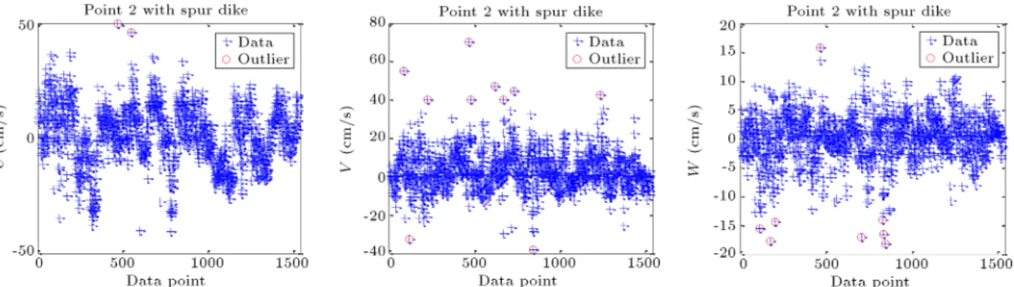
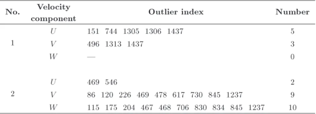
Table 2 provides the results of running Z-score test on the data sets. As obvious in the table, the maximum eect of the method is evident in Point 2 in both lateral and vertical directions. Moreover, outlier detection in such directions and at the downstream of spur dike extremely inuences the secondary ow strength variation and provides their true values at lower layers where the ow is exceedingly turbulent.
The outliers detected in the datasets are circled in Figure 4. This gure properly shows the necessity of outlier detection and its elimination from the time series of ow velocity components.
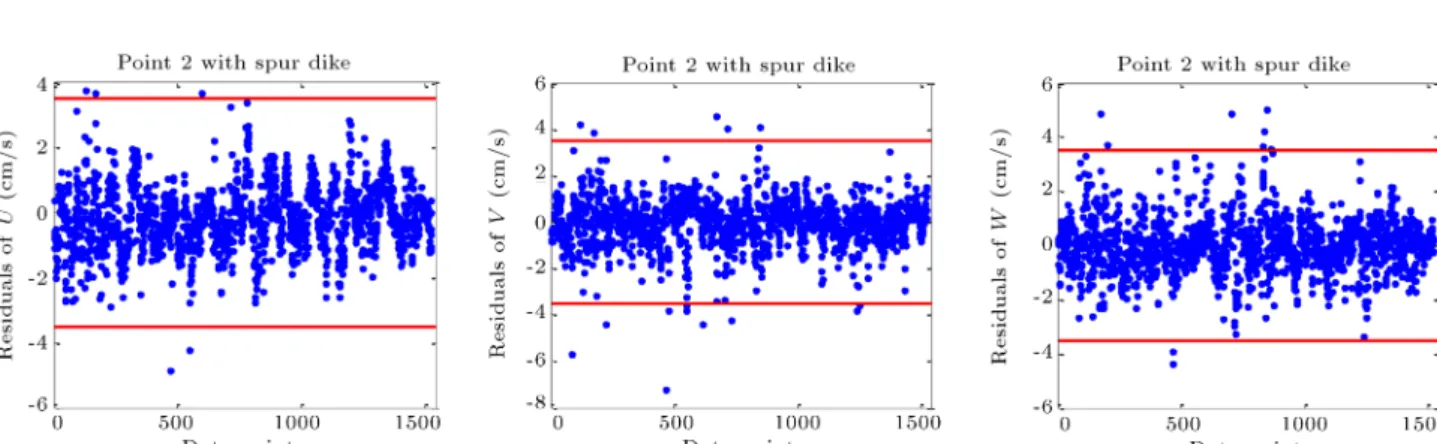
The results obtained thorough running curve t-ting method applying the sum of sines to the datasets are accessible in Table 3. By comparing Table 3 with Table 2, it can be stated that this method has marked more data as outlier candidates than Z-score. In order to indicate outlier detection using sum of sine curve tting, Figure 5 demonstrates the residuals of 3D velocity data after running the method on Point 2 as a dataset.
According to Figure 5, the sparsity of lateral velocity data due to higher turbulence and disorderly ow is estimated to be greater than those of the other two directions. Hence, the maximum number of the detected outliers related to lateral velocities in the experiment of bend with spur dike is identied by this strategy.
Table 4 presents details of the outlier detected through running the Mahalanobis on datasets. A point worth mentioning about Table 4 is that the results of this method are in accordance with those of Z-score test.
Table 4. Outliers detected in datasets using the Mahalanobis distance method. No. Velocity
component Outlier index Number
1
U 151 744 1305 1306 1437 5
V 496 1313 1437 3
W | 0
2
U 469 546 2
V 86 120 226 469 478 617 671 730 845 1237 10 W 115 175 204 468 706 830 834 845 1237 9
Figure 5. The residuals of the sum of sine curve tting (the horizontal line is the threshold parameter) in Point 2.
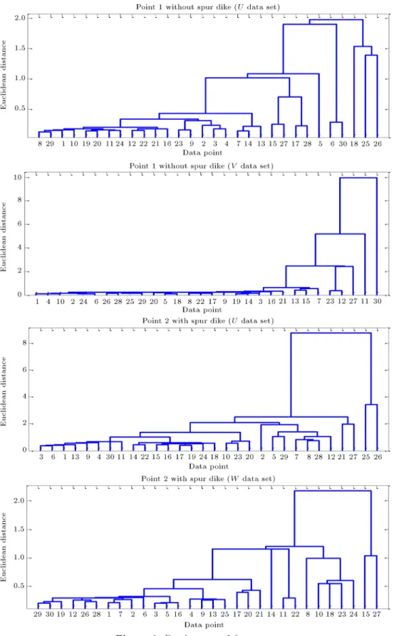
The results of running hierarchical clustering method on datasets are provided in Table 5, and cophenetic correlation coecient is given for each dataset, separately, in Table 5. As obvious in Table 5, this method fundamentally diers from the previous methods in terms of outlier detection through the ow pattern experiment along the bend (Point 1). Regarding the experiment with spur dike inside the bend, unlike previous methods, the longitudinal com-ponent of ow velocity bears the greatest proportion of outlier candidates. In addition, Figure 6 depicts the dendrogram of data sets. With regard to this gure and the comparison of correlation coecients provided in Table 6, it is evidently observed that the clustering tree and the reection of data of low coecient (such
as V in Point 1) and relatively appropriate coecients (such as W in Point 2) are in correlation. Since displaying all the indices on the horizontal axis in the dendrogram was impractical, the lower clusters were disregarded and only their 30 leaf nodes were represented. Consequently, some of the leaves in the diagram belong to more than one point.
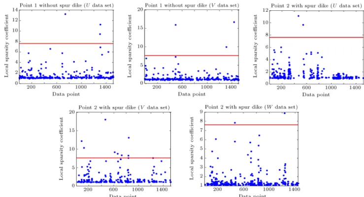
LSC-mine method results on data sets are shown in Table 7. A comparison between the results of this technique and the previous ones suggests that, by and large, the method has detected the minimum number of outliers in various directions.
Similarly, Figure 7 demonstrates the Local Spar-sity Coecient (LSC) values (data with a local sparSpar-sity ratio greater than the pruning factor (Pf)) in all the
Table 5. Outliers detected in datasets using hierarchical clustering method. No. Velocity
component Outlier index Number
1
U 1305 1306 744 151 1437 5
V 1313 23 497 496 1437 5
W 559 1193 2432 1431 872 1167 1511 7
2
U 45 46 70 74 86 186 188 549 558 671 676 845 317 598 779 469 546 17
V 226 478 617 671 730 1237 845 86 469 9
Figure 6. Dendrogram of data sets.
datasets along with the threshold limit value (horizon-tal line). The values falling above the horizon(horizon-tal line have been considered as the nal outlier candidates.
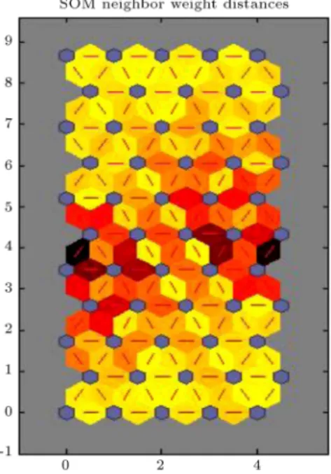
To cluster the input vector using self-organizing map, an 11-by-5 two-dimensional map of 55 neurons
is used. The two-dimensional map is of eleven by ve neurons, with distances calculated according to the link distance neighborhood function. Link distance is a layer distance function in MATLAB software used to nd the distances between the layer's neurons, given
Figure 7. Local Sparsity Coecient (LSC) for datasets. Table 6. Cophenetic correlation coecient calculated for
datasets.
No. Velocity component Cophenetic 1
U 0.509
V 0.3151
W 0.5386
2
U 0.4474
V 0.5837
W 0.6493
their positions. The two-dimensional self-organizing map has considered the topology of its inputs' space with parameters in Table 8. After training the SOM network, the data will be divided into 55 clusters. Here, as in fuzzy C-means clustering method, clusters whose
number of their members is less than 7 are considered as outlier candidates. Table 9 provides the results of running SOM on the data sets. Figure 8 indicates distances between neighboring neurons for Point 1, velocity component, U. This gure uses the following color coding:
The blue hexagons represent the neurons;
The red lines connect neighboring neurons;
The colors in the regions containing the red lines indicate the distances between neurons;
The darker colors represent larger distances;
The lighter colors represent smaller distances. Figure 9 shows how many data points are asso-ciated with each neuron. It is best if the data are distributed fairly and evenly across the neurons. In this example, overall, the distribution is fair even.
Table 7. Outliers detected in datasets using LSC-mine method. No. Velocity
component Outlier index Number
1
U 744 1305 1306 3
V 496 1313 1437 3
W | 3
2
U 469 546 2
V 86 120 469 617 668 730 841 845 8
Table 8. Self-organizing map network parameters.
Map dimensions 11 5
Number of neurons 55
Layer topology function Hexagonal
Neuron distance function Link distance function
Training algorithm Batch unsupervised weight/bias training Performance function Mean squared normalized error
Initial neighborhood size 3
Number of training steps for initial
covering of the input space 100
Number of epochs 200
Table 9. Outliers detected in datasets using self-organizing map method. No. Velocity
component Outlier index Number
1
U 744 1305 1306 151 1437 5
V 23 497 1313 496 1437 5
W 559 1193 1431 1432 1511 5
2
U 469 546 2
V 469 120 668 839 841 845 6
W 467 468 1237 3
Figure 8. Neural network training SOM neighbor weight distances for Point 1, velocity component U.
To apply the fuzzy C-means clustering method to a given dataset, it is needed to determine the number of clusters (C parameter), exponent for the partition matrix, maximum number of iterations, and minimum
Figure 9. Neural network training SOM sample hits for Point 1, velocity component U.
amount of improvement. In this research, C parameter value is selected by trial and error equal to 55. Other parameter values are as follows, respectively: 2.0, 1000, 1e-5. Clusters whose number of their members is less
Table 10. Outliers detected in datasets using fuzzy C-means clustering method. No. Velocity
component Outlier index Number
1
U | 0
V 13 159 299 540 960 1437 6
W | 0
2
U 45 46 70 549 558 845 6
V 187 706 828 1238 1252 5
W 467 468 669 717 721 1237 115 175 204 706 834 845 12
than 7 are considered as outlier candidates. Table 10 provides the results of running FCM on the data sets. Evidently, employing dierent approaches has led to various results. Some methods identied a data as an outlier, whereas the same sample was considered as normal by other techniques. Therefore, realizing whether a sample is a real outlier or not appeared to be a complicated problem; a substantial way to identify an outlier by the voting method. The outliers utilizing most of the methods can be potentially considered as outliers. In this way, the accuracy of the obtained results surprisingly increases.
In this paper, the samples marked as outliers in three methods are selected as the nal outlier candidates. In consideration of searching the points and calculating the frequency of each data, the binary search algorithm [28] is used. Table 11 presents the datasets' outlier identied by the voting method. Depending upon the nature of each algorithm, dier-ent methods result in various outcomes. One factor eective in the performance of each algorithm is taking correct parameters. To this end, it is attempted to select the best parameters for each algorithm regarding the nature of the data. As the voting method uses a comparability of the results obtained through the methods, its results can be taken as more accurate and reliable. In this study, further investigations have been based on the results (Table 11).
As seen in Table 11, Point 1 has fewer outliers
rather than Point 2. This is due to the installation of spur dike making the pattern of the turbulent ow around spur dike in the sharp bend more disorderly. Having detected outliers, they can be totally removed if there are few such data. Otherwise, they would be rectied or measured multiple times.
A noteworthy fact is that the outlier candidates chosen via such methods are not always indicative of error occurrence or fault in measurements. Perhaps, they are necessarily caused by variations of the system's nature circumstances (e.g., in ow conditions). The data may suggest an unknown behavior of the system under study so far. Indeed, detecting them can provide highly important information on the nature of the problem and lead to an even better understanding. Therefore, detecting outliers and the causes leading to such outliers must be investigated and the best approach be introduced; the strategy has been taken into account in this study.
In general, in this research, regarding various experiments, many critical factors probably involved in arising outliers are listed below:
Changes in ow condition;
Trivial uctuations of power and concluded eect on the discharge of the pump system;
Observational errors;
Spurious errors;
Systematic errors;
Table 11. Outliers detected in datasets using the voting method. No. Velocity
component Outlier index Number
1
U 151 744 1305 1306 1437 5
V 496 1313 1437 3
W | 0
2
U 469 546 2
V 86 120 226 469 478 617 730 845 1237 9 W 115 175 204 467 468 706 830 834 845 1237 10
Random errors;
Not following the correct measurement instructions;
Other factors such as environmental operative fac-tors, diculties with measurement devices, non-calibrated devices, human factors, such as optical illusions, the user's lack of experience and skill in using the measurement devices.
We should keep in mind that one method cannot always surpass other methods. One method may be eciently employed for a particular sort of data, while it is not ecient for another type. Therefore, this paper oers a process and while doing so, just the data selected by other methods as outliers are identied as the nal outlier candidates.
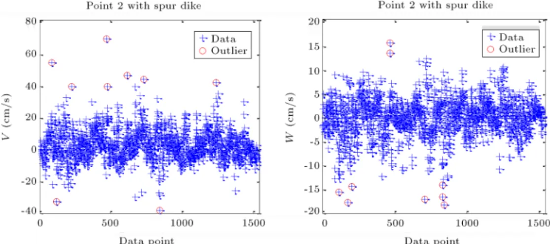
Figure 10 illustrates a dataset of vertical and lateral components of ow velocity in the case of bend with spur dike (Point 2) after running the voting method. As seen in the gure, employing the voting method integrates velocity time-series data and less disparity is evident through them.
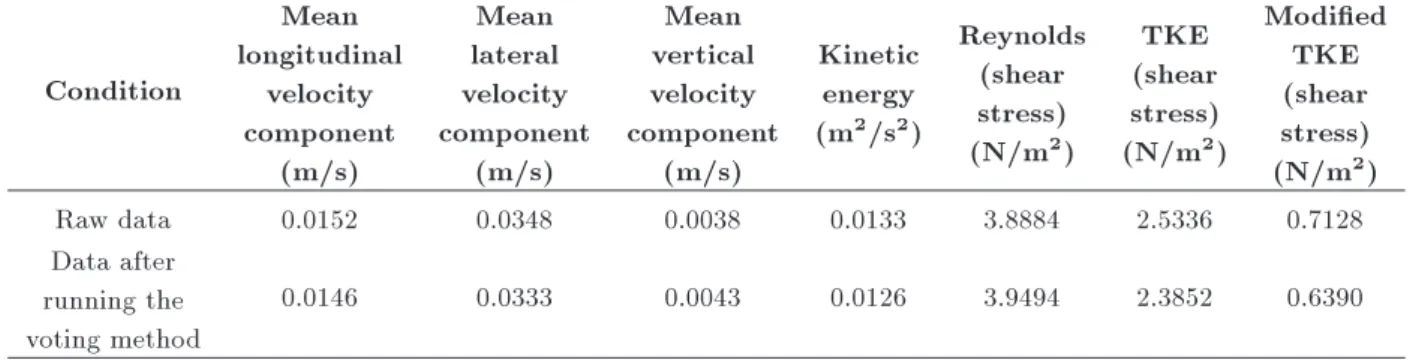
Concerning the accurate study of the eect of the detected outliers on ow pattern variations in the sharp bend, it is essential that dierent hydraulic parameters in turbulent ows be discussed. In Tables 12 and 13, kinetic energy and shear stress (using Reynolds [29],
TKE [30], and modied TKE [16,30]) parameters' values are compared with regard to the two considered points with and without a spur dike in the bend. Additionally, to observe mean ow pattern variations, the mean values of ow velocity components before and after outlier elimination from data sets are presented in these tables.
A noteworthy point in Table 12 is that after running the voting method on data sets, compared to other methods, the Reynolds shear stress parameter signicantly decreased by about 36%. Since there are no outliers reported in vertical direction in Table 11, the modied TKE before using voting method did not dier from the one after applying it. Overall, based on Table 12, it can be stated that in the case of the bend without a spur dike, running the voting method does not inuence the mean ow pattern aected by mean velocities, while 3D velocity components are signi-cantly exaggerated by spur dike installation at the bend apex, undergoing numerous variations. Considering Table 13, due to section constriction and a surge in ow velocity, in the centrifugal force and, subsequently, in the secondary ow strength, particularly at the downstream wing area (where Point 2 falls), a highly turbulent ow velocity will be dominant. As a result, it is not feasible to predict a certain order in ow patterns
Figure 10. The distribution of both lateral and vertical components of ow velocity by the voting method (Point 2). Table 12. A comparison between dierent hydraulic parameters governing the ow for the point without installation of spur dike in the bend (Point 1).
Condition
Mean longitudinal
velocity component
(m/s)
Mean lateral velocity component
(m/s)
Mean vertical velocity component
(m/s)
Kinetic energy (m2/s2)
Reynolds (shear stress) (N/m2)
TKE (shear stress) (N/m2)
Modied TKE (shear stress) (N/m2)
Raw data 0.4725 -0.0630 -0.0060 0.0022 0.4290 0.4270 0.3341
Data after running the voting method
Table 13. A comparison between dierent hydraulic parameters governing the ow for the point with spur dike in the bend (Point 2).
Condition Mean longitudinal velocity component (m/s) Mean lateral velocity component (m/s) Mean vertical velocity component (m/s) Kinetic energy (m2/s2)
Reynolds (shear stress) (N/m2)
TKE (shear stress) (N/m2)
Modied TKE (shear stress) (N/m2)
Raw data 0.0152 0.0348 0.0038 0.0133 3.8884 2.5336 0.7128
Data after running the voting method
0.0146 0.0333 0.0043 0.0126 3.9494 2.3852 0.6390
around spur dike. In spite of turbulence parameters, the mean ow parameters also undergo remarkable uctuations mainly found in resultant ow vertical component of strong up ows extant at downstream of the spur dike. According to Table 13, a 12% growth in vertical component at Point 2 reduced modied TKE, carried out using the voting system by 10%. Regarding other turbulence parameters, it can be said that running the voting method at Point 2 resulted in a decrease in all turbulence parameters except the Reynolds shear stress which increased by 1.5%.
4. Conclusion
Flow pattern analysis can provide highly important information on ow characteristics. Understanding the ow behavior under dierent circumstances can be achieved to some extent using experimental mea-surements. There are many causes of outliers in the measurements. Outliers may be produced by error of measurements or variations in the nature of the ow. Thus, detecting such data is vital from dierent viewpoints and can provide highly reliable results of the data. This paper employed a combination of Z-score test, sum of sines curve tting, Mahalanobis distance, hierarchical clustering, LSC-mine, self-organizing map, fuzzy C-means clustering, and voting methods to detect outliers in ow pattern experiments in a channel with a 180-degree bend with and without a T-shaped spur dike, individually. A comparison between dierent outlier detection methods indicates that one of the advantages of the voting method is that a compara-bility of the results of the other methods is applied and processed. It is highly recommended that before analyzing the collected data through ow pattern experiments, the procedure proposed in this paper be used in outlier detection. This paper has calculated dierent hydraulic parameters consisting of kinetic energy and shear stresses (using Reynolds, TKE, and modied TKE methods) in a bend with and without spur dike, and made comparison between them so as to study the impact of running the voting method on mean and turbulent ow pattern variations in a
sharp bend. Results showed that in the case of the bend without a spur dike, the mean velocities were not signicantly inuenced by the voting method, although it reduced the Reynolds shear stress by about 36%. Results were dierent in the case of the bend with a spur dike, and both mean and turbulence parameters of the ow underwent alterations, such that after the elimination of outliers detected through the voting method, under the inuence of installing the spur dike in the bend, a vertical velocity component faced a 12% growth, whereas modied TKE shear stress was decreased by 10%.
References
1. Basser, H., Karami, H., Shamshirband, S., Akib, S., Amirmojahedi, M., Ahmad, R., Jahangirzadeh, A., and Javidnia, H. \Hybrid ANFIS-PSO approach for predicting optimum parameters of a protective spur dike", Applied Soft Computing, 30, pp. 642-649 (2015).
2. Vaghe, M., Ghodsian, M., and Neyshabouri, S.A.A. \Experimental study on scour around a T-shaped spur dike in a channel bend", Journal of Hydraulic Engineering, 138(5), pp. 471-474 (2012).
3. Ghodsian, M. and Vaghe, M. \Experimental study on scour and ow eld in a scour hole around a T-shape spur dike in a 90 bend", International Journal of Sediment Research, 24(2), pp. 145-158 (2009).
4. Liao, T.W. \A clustering procedure for exploratory mining of vector time series", Pattern Recognition, 40(9), pp. 2550-2562 (2007).
5. Goring, D.G. and Nikora, V.I. \Despiking acoustic Doppler velocimeter data", Journal of Hydraulic En-gineering, 128(1), pp. 117-126 (2002).
6. Mori, N., Suzuki, T., and Kakuno, S. \Noise of acoustic Doppler velocimeter data in bubbly ows", Journal of Engineering Mechanics, 133(1), pp. 122-125 (2007).
7. Duncan, J., Dabiri, D., Hove, J., and Gharib, M. \Uni-versal outlier detection for particle image
velocime-try (PIV) and particle tracking velocimevelocime-try (PTV) data", Measurement Science and Technology, 21(5), p. 057002 (2010).
8. Westerweel, J. and Scarano, F. \Universal outlier detection for PIV data", Experiments in Fluids, 39(6), pp. 1096-1100 (2005).
9. Razaz, M. and Kawanisi, K. \Signal post-processing for acoustic velocimeters: detecting and replacing spikes", Measurement Science and Technology, 22(12), p. 125404 (2011).
10. Hawkins, D., Identication of Outliers, Chapman and Hall, London, UK (1980).
11. Filzmoser, P., Maronna, R., and Werner, M. \Out-lier identication in high dimensions", Computational Statistics and Data Analysis, 52, pp. 1694-1711 (2008).
12. Ramaswamy, S., Rastogi, R., and Kyuseok, S. \E-cient algorithms for mining outliers from large data sets", ACM SIGMOD Record, 29(2), pp. 93-104 (2000).
13. Hinneburg, A. and Keim, D.A. \An ecient approach to cluster in large multimedia databases with noise", SIGKDD, 98, pp. 12-19 (1998).
14. Hodge, V.J. and Austin, J. \A survey of outlier de-tection methodologies", Articial Intelligence Review, 22(2), pp. 85-126 (2004).
15. Leschziner, M.A. and Rodi, W. \Calculation of strongly curved open channel ow", Journal of Hy-draulic Division, 105(10), pp. 1297-1314 (1979).
16. Vaghe, M., Akbari, M., and Fiouz, A.R. \An exper-imental study of mean and turbulent ow in a 180 degree sharp open channel bend: Secondary ow and bed shear stress", KSCE Journal of Civil Engineering, 20(4), pp. 1582-1593 (2016).
17. Nortek, A.S., Vectrino Velocimeter User Guide, Nortek AS, Vangkroken, Norway (2009).
18. Schier, R.E. \Maximum Z Score and outliers", The American Statistician, 42(1), pp. 79-80 (1988).
19. Byrd, R.H. Schnabel, R.B., and Shultz, G.A. \Ap-proximate solution of the trust region problem by minimization over two-dimensional subspaces", Math-ematical Programming, 40(1), pp. 247-263 (1988).
20. Marquardt, D. \An algorithm for least-squares esti-mation of nonlinear parameters", SIAM Journal on Numerical Analysis, 11(2), pp. 431-441 (1963).
21. Gimenez, E., Crespi, M., Garrido, M.S., and Gil, A.J. \Multivariate outlier detection based on robust computation of Mahalanobis distances application to positioning assisted by RTK GNSS Networks",
In-ternational Journal of Applied Earth Observation and Geoinformation, 16, pp. 94-100 (2012).
22. Liao, T.W. \Clustering of time series data-a survey", Pattern Recognition, 38, pp. 1857-1874 (2005).
23. De Morsier, F., Tuia, D., Borgeaud, M., Gass, V., and Thiran, J.P. \Cluster validity measure and merging system for hierarchical clustering considering outliers", Pattern Recognition, 48(4), pp. 1478-1489 (2015).
24. Farris, J.S. \On the cophenetic correlation coecient", Systematic Biology, 18(3), pp. 279-285 (1969).
25. Agyemang, M. and Ezeife, C.I. \LSC Mine: algorithm for mining local outliers", 15th Information Resources Management Association, New Orleans, USA, pp. 23-26 (2004).
26. Kohonen, T., Self-Organizing Maps, Springer, New York, USA (1997).
27. Kaufman, L. and Rousseeuw, P.J., Finding Groups in Data: an Introduction to Cluster Analysis, John Wiley & Sons, New York, USA (1990).
28. Cormen, T.H., Leiserson, E.C., and Rivest, R.L., Introduction to Algorithms, 1st Edn., McGraw-Hill, New York, USA (1990).
29. Barbhuiya, A.K. and Dey, S. \Measurement of tur-bulent ow eld at a vertical semicircular cylinder attached to the sidewall of a rectangular channel", Flow Measurement and Instrumentation, 15(2), pp. 87-96 (2004).
30. Kim, S.C., Friedrichs, C.T., Maa, J.Y., and Wright, L.D. \Estimating bottom stress in tidal boundary layer from acoustic Doppler velocimeter data", Journal of Hydraulic Engineering, 126(6), pp. 399-406 (2000).
Biographies
Mohammad Vaghe received his BSc and MSc de-gree in Civil Engineering from Shiraz University (Iran). He earned his PhD in Hydraulic Structures from Tar-biat Modares University (Iran) in 2009. His research in-terests are in the elds of Numerical and Experimental Methods in Hydraulic Structures, River Engineering, and Hydrodynamics. He has presented 220 papers at national and international conferences and has pub-lished 120 journal papers. He is currently an Associate Professor at Persian Gulf University, Bushehr, Iran. Kumars Mahmoodi received his BSc degree in Civil Engineering from Persian Gulf University in Bushehr (Iran) in 2012; he also earned his MSc degree in Coastal Engineering from Amirkabir University of Technology (Iran) in 2014. He is mainly interested in computer sciences, data mining, programming, numerical methods in marine and hydraulic engineering, sediment transport, and coastal structures. He is the author of 3 published papers in journals and 22 presented papers at conferences. Also, he wrote a
reference book on C Programming Language.
Maryam Akbari earned her BSc and MSc degrees in Civil Engineering from Persian Gulf University, Bushehr (Iran) in 2012 and 2015, correspondingly. Her research interests are in the areas of hydraulic
struc-tures, hydrodynamics, and experimental and numerical modeling. She is the author and co-author of 15 published papers at national and international journals and 6 presented papers at conferences. She is currently a lecturer in Civil Engineering Department, Persian Gulf University, Bushehr, Iran.