Open Journal Systems

(1)

ORIGINAL ARTICLE

Research on Treasury Bond Futures Trading Strategy Based on

ARIMA Model

Zihan Zhang*

School of Finance, Central University of Finance and Economics, Beijing 102206, China. E-mail: [email protected]

Abstract: This paper uses the ARIMA model to analyze the yield to maturity of China’s 10-year Treasury Bonds, and uses this yield rate to establish an investment strategy for 10-year Treasury Bond Futures (continuous in the current quarter). And then the strategy was back-tested in periods. In this paper, firstly, based on the ARIMA model, the full-sample fitting of the 10-year Treasury Bond yield to maturity series is carried out, and the fitting effect is confirmed. Then, the signal indicators and position sequence are established by comparing the iterative predicted value and the observed value. According to this method, the investment process of Treasury Bond Futures is simulated, and the return change of the strategy is quantified. Back-testing shows that this strategy tends to perform better in the volatile and bear market periods of the bond market but to underperform in the bull market period.

Keywords: Treasury Bond Yield to Maturity; Treasury Bond Futures; ARIMA Model; Trading Strategy

1. Hypothesis of research

The 10-year Treasury Bond yield to maturity is used as an indicator for investment transactions, and other indica-tors are not considered in this research. Therefore, the main idea of this strategy is to construct a suitable trading sig-nal by modeling and asig-nalyzing the time series of the 10-year Treasury Bond’s yield to maturity, and then it simulates trading according to the instructions of the signal and back-test its effect.

The specific investment target selected is the 10-year China’s Treasury Bond Futures (continuous in the current quarter), of which the logic will be discussed below. The price curve of this target has good smoothness and it is suitable for research.

Considering the availability and completeness of the data and the complexity of model processing, it is assumed that the highest transaction frequency of the above investment targets by investors is the daily frequency, and the trans-action price is set to the closing price of the current day regardless of the long or short transtrans-action.

2. Sample fitting based on ARIMA model

2.1 Sample space

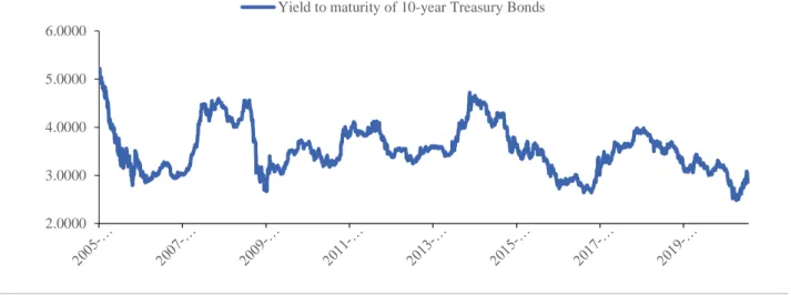
The yield to maturity data of 10-year Treasury Bonds from January 1, 2005 to July 24, 2020 is obtained. The trend is shown in the figure below.

This is an open-access article distributed under the terms of the Creative Commons Attribution Non-Commercial License

(2)

Figure 1. Yield to maturity of 10-year Treasury Bonds.

2.2 Construction of ARIMA model

First, the stationarity test of the return to maturity (TB_YTM) series is performed. The DF test result shows that the series can be considered as stable at the 5% significance level, so no difference is needed. ARMA model can be di-rectly applied, namely ARIMA (p, 0, q).

Variable Statistic P-value

TB_YTM -3.276 0.0160

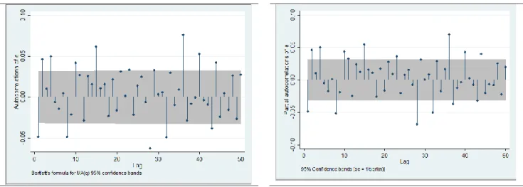
In order to determine the lag order p and q of AR and MA, we draw the ACF and PACF diagrams of YTM. The ACF chart is obviously tailing, indicating that q=0, while the PACF chart is truncated. From the graphical observation, it seems that AR (1) and AR (2) are both reasonable.

For further judgment, its AIC and BIC indicators are calculated.

Model AIC BIC

AR(1) -1599.398 -1587.610

AR(2) -1602.256 -1586.537

AIC and BIC have certain differences in parameter selection. Considering that BIC’s penalty for loss of freedom may be slightly severe, AR (2) is selected according to the value of AIC index.

In summary, the model we actually chose is ARIMA (2, 0, 0).

Figure 2. ACF graph of TB_YTM. Figure 3. PACF graph of TB_YTM. 2.0000

3.0000 4.0000 5.0000 6.0000

(3)

In addition, we need to check whether the residual sequence has autocorrelation. Actually, the ACF and PACF dia-grams show that there is no significant sequence correlation problem. And the result of DW test is that there is no serial correlation. Therefore, the model is effective enough.

Figure 4. ACF graph of residual sequence Figure 5. PACF graph of residual sequence

2.3 Fitting effect of ARIMA model

Figure 6. Fitting of the ARIMA model to the entire sample.

Judging from the graph above, the ARIMA model fits the change trend of TB_YTM quite accurately. To be more accurate, the MAE (Mean Absolute Error) and MER (Mean Error Rate) are shown as follows.

𝑀𝐴𝐸 =1

𝑁∑ |𝑌𝑇𝑀̂ − 𝑌𝑇𝑀| = 0.02135

𝑀𝐸𝑅 =1

𝑁∑

|𝑌𝑇𝑀̂ − 𝑌𝑇𝑀|

𝑌𝑇𝑀 = 0.612%

The MAE of this model is 0.02135, and the MER is 0.612%, which shows that the model has a good capacity of error control.

3. Iterative forecast based on ARIMA model

3.1 Iterative forecast method

The research in the last part basically confirmed the rationality and reliability of the ARIMA model for time series modeling and analysis.

2.0000 3.0000 4.0000 5.0000 6.0000

TB_YTM observed value

(4)

But logically, the fitting done in the previous part is actually based on the intra-sample prediction of the entire sample. In practical forecasting, at the current point in time, it is meaningless to “predict” history based on known in-formation, and it is impossible to “predict” immediate changes based on long-term information. Therefore, we should use a more scientific and rigorous method for prediction, that is, iterative out-of-sample forecast based on information updates.

The method of iterative forecast is to select the n-th (1 < n < N) period as the starting point of the iteration. It fits an appropriate model based on the data observations from the 1st to the n-th period and use the model to predict the n+1th period. Furthermore, after the information of the sequence is updated in the n+1 period, a new model is fit-ted based on the data observations from the 1st period to the n+1 period, and the data of the n+2 period is predicfit-ted; and so on to predict to the N-th period. Although we still use the same sample space, iterative forecasting continuously uses historical information when making forecasts at each time point, so it is essentially a dynamic out-of-sample forecast, which is more in line with the logic of forecasting in practice.

3.2 Effect of iterative forecast

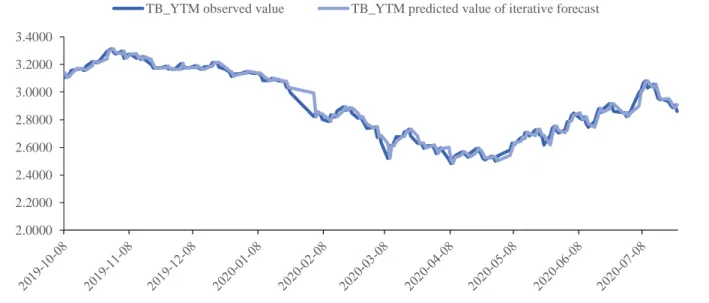
In the study of the 10-year Treasury Bond yield sequence, the starting time of iterative forecasting was selected on September 30, 2019, and the iterative forecasting was applied till July 22, 2020. Because this process requires continu-ous fitting and updating of the model every trading day, the relevant tests are omitted here. The forecast effect is shown in the figure below.

Figure 7. Iterative forecast of ARIMA model.

Refer to the formulas in the above section to calculate the Mean Absolute Error (MAE) as 0.02356 and the Mean Error Rate (MER) as 0.833%. This result is slightly higher than the error rate of the in-sample forecast, which is rea-sonable, and it more truly reflects the process of continuous updating of information in a sequence over time.

4. Construction of signal indicators and position sequence

4.1 Basic logic

Firstly, let us briefly discuss why the 10-year Treasury Bond yield to maturity is used as an indicator to indicate the trading of Treasury Bond Futures.

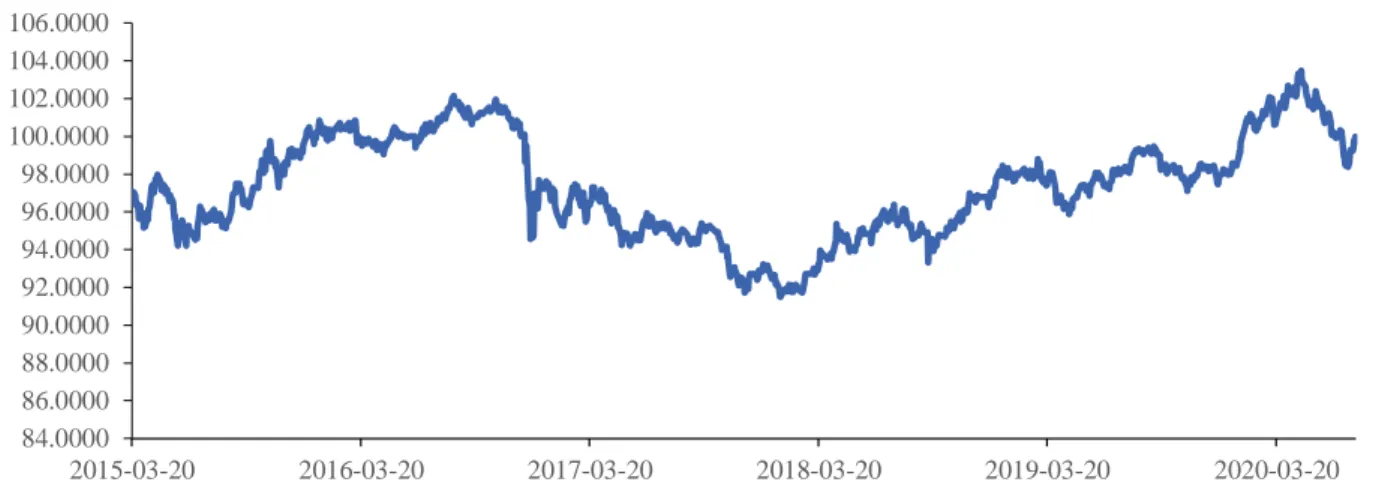
Trend of 10-year Treasury Bond Futures (continuous in the current quarter) from March 20, 2015 to the present is shown in the chart below.

2.0000 2.2000 2.4000 2.6000 2.8000 3.0000 3.2000 3.4000

(5)

Figure 8. Trend of 10-year Treasury Bond Futures (continuous in the current quarter).

From a logical analysis, since the yield to maturity of the Treasury Bond is essentially a discount rate, the price of the national debt futures will inevitably show a reverse change. From an empirical point of view and the correlation analysis between Treasury Bond Futures and Treasury Bond yields from March 20, 2015 until now, the correlation co-efficient is -0.9869, so Treasury Bond yields to maturity can be used as a good reflection of Treasury Bond Futures trading. In other words, the basic idea is to long Treasury Bond Futures when the yield to maturity of Treasury Bonds is expected to fall, and short Treasury Bond Futures when the yield to maturity of Treasury Bonds is expected to rise.

4.2 Construction of signal indicator

The focus of constructing signal indicators is the difference between the observed value and the predicted value of the ARIMA model. The predicted value given by the ARIMA model retains more of the inertia of historical information. Therefore, when the observed value curve passes through the predicted value curve from the lower to the upper side, it means that there is a short-term upward trend that breaks through inertia, and when the observed value curve crosses from the upper direction to the lower direction of the predicted value curve, it means that there is a short-term down-ward trend which breaks through inertia. At the same time, because the sequence itself is stationary and the ARIMA model is effective in modeling, when the observed value curve crosses the predicted value curve in a certain direction, the observed value curve will inevitably not diverge, but it will return to the predicted value curve again to form the next intersection.

Since a stronger yield to maturity of Treasury Bonds means a weaker Treasury Bond Futures prices, and vice versa, the signals indicators are as follows:

(1) Long signal:𝑌𝑇𝑀_𝑡−1≥ 𝑌𝑇𝑀̂ & 𝑌𝑇𝑀_𝑡−1 _𝑡< 𝑌𝑇𝑀̂_𝑡

(2) Short signal:𝑌𝑇𝑀_𝑡−1 ≤ 𝑌𝑇𝑀̂ & 𝑌𝑇𝑀_𝑡−1 _𝑡> 𝑌𝑇𝑀̂_𝑡

Since the observed value and predicted value curves are smooth, and the real numbers have tri-ambiguity, buying signals and selling signals must appear alternately.

4.3 Construction of position sequence

Based on the above analysis, we should go long Treasury Bond Futures when a long signal appears, and short Treasury Bond Futures when a short signal appears. After one signal appears, before the next signal appears, the posi-tion direcposi-tion indicated by the last signal should be maintained.

In detail, the position sequence is 1 for holding a long position, and -1 for holding a short position. If a long signal appears on day t, the value of the position sequence from day t+1 to the day when the next short signal appears is 1; if a short signal appears on day t, then from t+1 to the next long signal, the value of the position sequence on the day of oc-currence is -1. And so on.

84.0000 86.0000 88.0000 90.0000 92.0000 94.0000 96.0000 98.0000 100.0000 102.0000 104.0000 106.0000

2015-03-20 2016-03-20 2017-03-20 2018-03-20 2019-03-20 2020-03-20 Trend of 10-year Treasury Bond Futures (continuous in the current quarter)

(6)

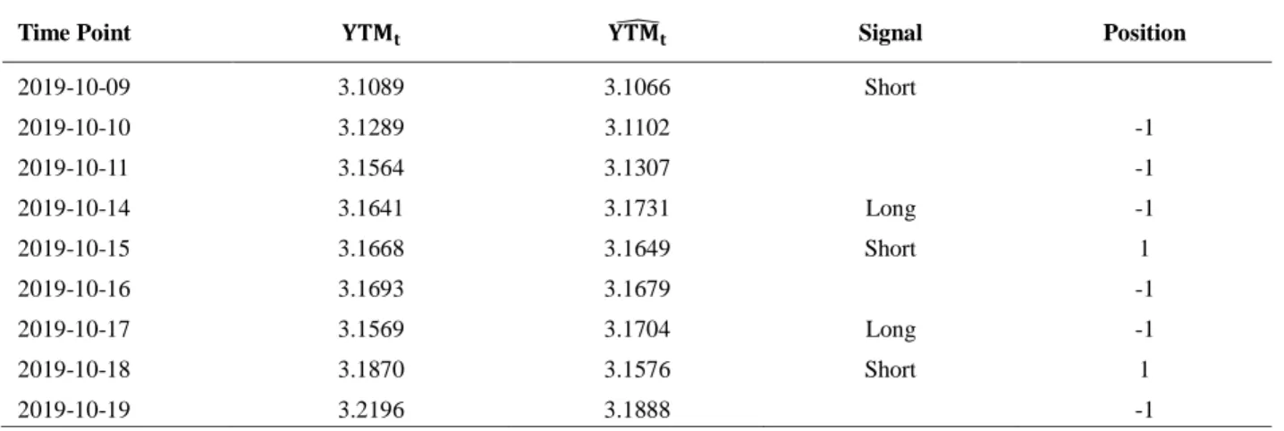
Taking the interval from October 9, 2019 to October 19, 2019 as an example, the trend of TB_YTM observations and forecasts, signal conditions and position sequence values are illustrated in the following table.

Time Point 𝐘𝐓𝐌𝐭 𝐘𝐓𝐌𝐭̂ Signal Position

2019-10-09 3.1089 3.1066 Short

2019-10-10 3.1289 3.1102 -1

2019-10-11 3.1564 3.1307 -1

2019-10-14 3.1641 3.1731 Long -1

2019-10-15 3.1668 3.1649 Short 1

2019-10-16 3.1693 3.1679 -1

2019-10-17 3.1569 3.1704 Long -1

2019-10-18 3.1870 3.1576 Short 1

2019-10-19 3.2196 3.1888 -1

5. Strategy backtest

5.1 Calculation of cumulative return rate

According to China’s futures trading system, assuming the Treasury Bond Futures transaction rate is 5‰, the cu-mulative return rate on the t (t > 2) day after the start of the test investment is:

𝐶𝑅 = 1

10000(10000 ∗ ∏ 𝑝𝑜𝑠𝑖𝑡𝑖𝑜𝑛𝑖∗ (1 + 𝑟𝑖)

𝑡

𝑖=1

− count(𝑠𝑖𝑔𝑛𝑎𝑙) + 0.5)

Among them, 𝑝𝑜𝑠𝑖𝑡𝑖𝑜𝑛𝑖 is the i-th number of position sequence, 𝑟𝑖 is the i-th number of the sequence of the

fu-tures price change rate on a single day, and count(𝑠𝑖𝑔𝑛𝑎𝑙) represents the number of signals (no matter long or short) that appear in a period of time. It should be pointed out that during a period of time, the initial signal only means mak-ing one transaction, while the followmak-ing signal is to do a backhand transaction, that is, two transactions for closmak-ing and opening positions.

5.2 Back-testing in different situations

The reference standard is set as the interval cumulative return rate for buying and holding Treasury Bond Futures, and the following back-testing is done in different periods.

(1) Shock period (2019.10.09-2020.01.07), the cumulative yield curve in this interval is:

Figure 9. Strategy returns during the shock period. -1.50%

-1.00% -0.50% 0.00% 0.50% 1.00% 1.50%

(7)

The comparison of strategy and benchmark is:

Interval Cumulative Rate

of Return Maximum Drawdown Daily win rate

Strategy 0.72% -1.90% 51.61%

Benchmark -0.46% -1.11% 45.16%

It can be seen that the strategy has stronger profitability and higher winning rate than the benchmark, but the risk of retracement is greater.

(2) Bull market period (2020.01.08-2020.04.30), the cumulative yield curve in this interval is:

Figure 10. Strategy returns during the bull market period.

Strategy 1.45% -1.43% 50.68%

Benchmark 4.92% -1.42% 57.53%

It can be seen that the strategy performs poorly during the bull market, with returns lower than the benchmark and risks higher than the benchmark.

(3) Bull market period (2020.05.11-2020.07.17), the cumulative yield curve in this interval is:

Figure 11. Strategy returns during the bear market period. 0.00%

1.00% 2.00% 3.00% 4.00% 5.00% 6.00%

Strategy cumulative return Benchmark cumulative return

-4.00% -3.00% -2.00% -1.00% 0.00% 1.00% 2.00% 3.00%

(8)

Strategy 2.14% -0.60% 48.89%

Benchmark -2.42% -3.92% 48.89%

It’s obvious that the strategy performs better than the benchmark in terms of both returns and risks, and it has ob-vious advantages.

6. Conclusion

According to the above back-testing results, this strategy tends to perform better in the bear market and shock pe-riods of the bond market and outperform the benchmark. This is mainly because frequent “arbitrage” generates more returns, and at the same time it avoids the substantial loss of simply holding long positions. However, in the bull market period, frequent transactions generate excessive costs, which is not as cost-effective as buying and holding.

References

1. Dong C. Bond quantitative trading operation method and evaluation using homeopathic indicators (in Chinese). China Bond 2019; (6).

2. Ding L, Chen M, Zou P. The empirical research on the price discovery function of Treasury Bond Future in China (in Chinese). Chemical Engineering Transactions 2015; (46).

3. Chen J. Bond pricing and yield curve modeling: A structural approach (in Chinese). Quantitative Finance 2020; (20).

4. Lu L. Combinational stock price forecasting based on multiple regression and technical analysis. Journal of Shanghai Institute of Technology (Natural Science) 2014; 14(3): 274–276.

5. Koijen RSJ, Lustig H, Stijn VN. The cross-section and time-series of stock and bond returns. Journal of Monetary Economics 2017; 88: 50–69.

6. Wang J, Tang S. Time series classification based on arima and adaboost. MATEC Web of Conferences 2020; 309(2): 03024.