ABSTRACT
KUEN-YUH WU. Spatial and temporal variations of bioaerosol concentrations. (Under The Direction of Dr. Russell W. Wiener)
Investigating microbiological contaminants in an environment is usually conducted by air sampling. Collection of representative samples in the environment may serve several functions, such as specification of species and sources, verification of control action, and accomplishment of the long-term goal to relate bioaerosol exposure to human health risk. However, the bioaerosol concentrations usually exhibit temporal, and spatial variations. These variations highly affect determination of representative samples in the environment. The study of temporal and spatial variations was conducted in three environments, two indoor sites within an office and laboratory research building and one outdoor adjacent site. The Andersen two-stage samplers were used to
collect bacteria. A hot-film anemometer were used to measure
air velocity in these two indoor sites. Bacterial samples were grown on TSA agar and incubated at 3 0°C for three days. The colony-formed units were counted. The counts were used to statistically study the relationship between the tested parameters (temperature, relative humidity,and air velocity)
and the collected bacterial concentrations. Variations in
TABLE OF CONTENT
ABSTRACT
TABLE OF CONTENT iii
LIST OF ABBREVIATION IIX
LISTS OF TABLES ix LISTS OF FIGURES xiii I. INTRODUCTION ixv
A. General Description ixv B. Definition of Bioaerosols 3 C. Bioaerosol and Indoor Air Quality 3 D. Bioaerosols and Health Effects 4 1. Allergy 4 2. Infectious diseases 5 E. Risk Assessment and Bioaerosols 6
F. The Intrinsic Complexities of Sampling Bioaerosols 7 G. Factors Associated with Sampling Bioaerosols 8 H. The Objectives of this Study 9
II.BACKGROUND AND LITERATURE REVIEW 14 A. Brief History of Sampling Bioaerosols 14 B. Review and Comparison of Bioaerosol Samplers 15 C. The Guidelines Published by the ACGIH Committee 19 D. Spatial and Temporal Variation for Exposure
III. METHODOLOGY AND EXPERIMENTS CONDUCTED 23
A. Sampling Bioaerosols 23 1. Sampling Location 23
2. Selection of Bioaerosol Samplers 23 3. Calibration of the Andersen Two-Stage Microbial
Samplers 24
4. Sampler Arrangement 25 5. Selection of Media (agar) 26 6. Preparation of Agar Plates 26 7. Sampling for Comparison of the Intra-Paired
Variation of Collected Bioaerosol
Concentrations 27
8. Sampling Procedures 29 B. Measurement of Air Movement 30
1. Instrument 30 2. Calibration of the Omnidirectional Probe 32
3. Procedures for Measuring Air Velocity 35
4. Measurement of Air Movement with a Single Probe 37
a) Measurement in the Nonventilated Room 37 b) Measurement in Room S-250 37 5. Synchronization of Collection of Bioaerosols
with Measurement of Air Movement 38
C. Data Analysis 39 1. Non-parametric Statistical Method 39 2. Analysis Based on Log-Normal Distribution 41
3. Test Based on Normal Distribution 41
4. Spatial Statistics 42 5. Temporal Variation 43
IV. RESULTS 45 A. Calibration of the Andersen Two-Stage Samplers 45
B. Comparison of the Intra-Paired Variation 45 C. Temporal and Spatial Variation for the Total Counts
1. Samples Collected in the Stairwell 49 2. Samples Collected in the Outdoor Environment 57 3. Samples Collected in the Ventilated Room 59
4. Samples Collected during the Day in the
Nonventilated Room 60 D. Respirable and Irrespirable Counts 63 1. Respirable Counts 66 2. Irrespirable Counts 66
E. Measurement of Air Movement 74
1. Calibration of Hot-wire Probes 74
2. Measurement of Air Movement in the Room S-250
Nonventilated Environment
4. Simultaneously Collecting Bioaerosols
and Measuring Air Movement in Room S-250 91
V DISCUSSION 94 A. Calibration of the Andersen Samplers 94 B. Intra-Paired Variation 95 C. Total Counts 96
1. Samples Collected in the Stairway without Human Activity 96 a. Temporal Variation 96
b. Spatial Variation 99 2. Samples Collected on the Roof of the Annex
Building 101 3. Samples Collected in the Ventilated Room
(S-250) 102
a. Spatial Variation 102 b. Temporal Variation 103 4. The Relationship between Collected Bacterial
Concentrations and Temperature and Relative Humidity 104
6. Sampler Arrangement 108 D. Respirable and Irrespirable Counts 110 1. Respirable Counts 110 2. Irrespirable Counts 112
E. Air Movement and Bacterial Concentration 113
1. Measurement of Air Movement 113 2. Simultaneous Collection of Bacteria and
Measurement of Air Movement 115
a. Air Velocity and Collected Bacterial
Concentrations 115 b. Spatial Variation and Air Velocity 118 VI. CONCLUSIONS 120
VII. FUTURE WORKS 123
LIST OF TABLES
1. Air velocity corresponding to the pressure drop for
calibration of the omindirectional probe. 3 6
2. Calibration of the critical flow rate for the Andersen
two stage sampler (pump air into the gasometer), 46
3. Calibration of the critical flow rate for the Andersen
two stage sampler (suck air out of the gasometer). 47 4. Calibration of flow rate for the Andersen two stage
sampler (suck air out of the gasometer). 47 5. Comparison of collection efficiency of the Andersen
two-stage sampler at different critical flow rate. 48 6. An example for the t test and distribution-free sign
test. 51
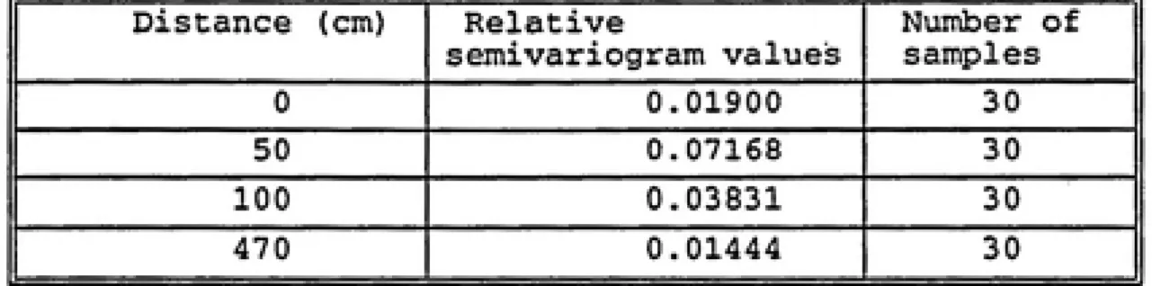
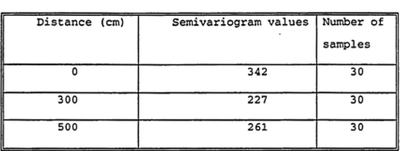
7. The comparison of spatial variation of samples collected at different distances between two samplers with
semivariogram and relative semivariogram values. 54 8. Variance component for samples collected in the room
without ventilation (data transformed to log scale). 56 9. The comparison of semivariogram values for samples
collected simultaneously by four samplers on the roof of the Annex Building. 58
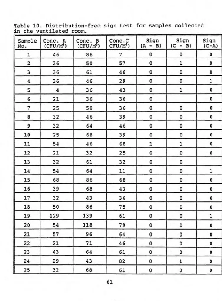
10. Distribution-free sign test for samples collected in the
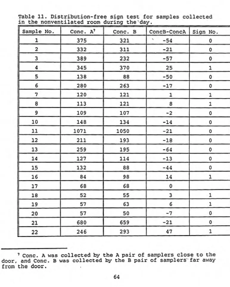
11. Distribution-free sign test for samples collected in the
nonventilated room during the day. 64
12. Relative semivariogram values for respirable counts
(samples collected in the stairwell). 67
13. Spatial variation for respirable counts (samples
collected in the ventilated room). 68
14. Spatial variation for respirable counts (samples
collected in the outdoor environment). 69
15. Comparison of spatial variation between respirable counts
and irrespirable counts for samples collected in the
stairwell. 70
16. Comparison of spatial variation between respirable
counts and irrespirable counts for the outdoor samples.71 17. Spatial variation with distribution-free sign test
(samples were collected in the ventilated room). 72
18. Spatial variation with distribution-free sign test for
samples collected at stairwell during the day. 75
19. The calibration data for the first probe. 77 20. The calibration data for the second probe. 78 21. Air conditioner on but hoods off (Air velocity was
measured at the door of the room S-250). 79
22. Air conditioner and hoods on (Air velocity was measured
measured at the middle of the room S-250) . 81
24. Air conditioner and hoods on (Air velocity was measured
at the middle of the room S-250). 81 25. Air conditioner and hoods off (Air velocity was measured
deep inside the room S-250). 83 26. Air conditioner off but hoods on (Air velocity was
measured deep inside the room S-250). 83
27. Air conditioner and hoods off (Air velocity was measured
at the door of the room S-250) . 84 28. Air conditioner off but hoods on (Air velocity was
measured at the door of the room S-250) . 84
29. Air conditioner and hoods off (Air velocity was measured
at the middle of the room S-250). 86
30. Air conditioner and hoods off (Air velocity was measured
at the middle of the room S-250). 86
31. Air conditioner on but hoods off (Air velocity was
measured deep inside the room S-250). 87 32. Air conditioner and hoods on (Air velocity was measured
deep inside the room S-250). 87
33. Still air in the stairwell at the basement. 89
34. Measurement of air movement close to the door 90
35. Measurement of air movement close to the door 9 0
36. Measurement of air movement far away from the door 92
LIST OF FIGURES
1. Sampler arrangement in the indoor environment with no ventilation 131 2. Sampler arrangement in the outdoor environment 131
3. Sampler arrangement in the indoor environment with a
ventilation system 131 4. Pattern of temporal variation in bioaerosol concentration
collected indoors without human activity and
ventilation 131
5. The layout for calibration of the Andersen two-stage
sampler --- pumping air out of a gasometer 132 6. The layout for calibration of the Andersen two-stage
sampler --- pumping air into a gasometer 133
7. The layout for simultaneously sampling bacteria and
measuring air velocity 134 8. The relationship between logarithm of bacterial
concentrations and temperature (samples are collected in
the nonventilated environment) 13 5
9. The relationship between logarithm of bacterial
concentrations and relative humidity (samples are collected in the nonventilated environment) 13 6
11. Bacterial concentration v.s. time (samples were collected
outdoors) 138
12. Bacterial concentrations v.s. time (samples were collected
in the room S-250) 13 9
13. Bacterial concentrations v.s. time (samples were collected during the day) 140 14. The calibration curve for the first probe 141 15. The calibration curve for the second probe 142 16. Bacterial concentrations v.s. air velocity (samples were
collected in the room S-250) 143
17. RMS v.s. air velocity (the probe was 110 cm off floor) 144 18. Bacterial concentrations v.s. RMS (samples were collected
in the room S-250) 145
19. Bacterial concentration v.s. turbulence intensity 146 20. Spatial variation and the condition of air movement 147 21. The distribution of mean air velocity at each condition of
air movement 148
22. The distribution of RMS at each conditions of air movement
149
I. INTRODUCTION A. General description
Bioaerosols were responsible for the outbreak of
Legionnaires' disease which caused 29 deaths in Philadelphia in 1976 (J.C. Feeley 1988). Bioaerosols also have been
linked to complaints of illnesses by occupants of tightly sealed building (P.S. Hockaday 1988 and Wallingford. 1986).
Investigations of the outbreak of Legionnaires' disease and
building-associated symptoms have been conducted by air sampling to find the etiological agents.
Air sampling may contain short-term and long-term
objectives. The short term objectives include; 1)
identifying bioaerosol species, 2) identifying sources of bioaerosols, and 3) providing means to monitor corrective
procedures. The long-term objective is to relate health
risk to bioaerosol exposure,
A number of sampling difficulties exist related to attaining representative bioaerosol samples including the
following:
1. No personal sampler, with high collection efficiency,_
is currently available.
">^:^'!;?^^^'/^-f^^^s%^^^5^"^^
2. Desiccation of the collected microorganisms in the
sampler results in underestimation of bioaerosol
concentration (C.S. Cox, 1988).
3. For the all-glass liquid impingers (AGI), loss of water due to the long sampling time may result in
overestimation of microbial concentration.
4. Bioaerosol concentration in an environment may vary with time (temporal variation^) and with locations
(spatial variation^).
Facing these difficulties, investigators usually estimate
bioaerosol concentration using short-term sampling at a fixed location in an environment. Bioaerosol concentrations usually exhibit temporal and spatial variations at the sampling location. Due to the temporal and spatial variations,
estimation of bioaerosol concentrations challenges investigators (or industrial hygienists).
Accurate estimation of bioaerosol concentrations should be
based on collection of representative samples in an
^. Variation associated with sampling different times at the
same location.
environment. Representative samples may be collected by
understanding temporal and spatial variations, and determining
the factors associated with these variations in an
environment. This study investigates temporal and spatial variation in three environments. The relationships between bioaerosol concentrations and temperature, relative humidity, and air velocity are tested in these environments.
B. Definition of bioaerosols
The American Council of Government and Industrial Hygiene (ACGIH) defines bioaerosols as airborne microorganisms, large
molecules or volatile compounds that are released from a living organism (M.A. Chatigny and J.M. Macher, 1989). Airborne microorganisms may include bacteria, fungi, viruses,
and protozoa. Bacterial, fungi, and protozoa are also called viable particles (aerosols) since they can reproduce
themselves at extracellular state. Other particles are called
nonviable particles. Antigens and endotoxins are two major molecular components in bioaerosols. The particle size of
bioaerosols varies from less than 0.1 |im to greater than 100 um,
C. Bioaerosols and indoor air quality
the production and transport of biological aerosols.
Reservoirs within an environment provide a set of conditions
in which microorganisms survive. Amplifiers allow the microorganisms to multiply. Disseminators act to introduce the microorganisms and their metabolites into the air. The primary requirement for the growth and amplification of microorganisms in the indoor environment is the presence of
moisture which can occur in a building regardless of the amount of outdoor air being supplied to the space (P.R. Morey
1987)
In an indoor environment, not only airborne microorganisms but also their derivatives could be potential hazards to residents. Antigens could be derived from microorganisms, arthropods, or animals. Endotoxins are excreta of bacteria and molds. Fungi excrete mycotoxin. Antigens, endotoxins, and mycotoxins are also potential health hazards for residents.
Microorganisms also produce volatile organic compounds and
cause odor problems in indoor environments.
D. Bioaerosols and health effects:
Bioaerosols in the indoor environment may cause allergy
and infectious illnesses. 1. Allergy
may result from exposure to allergens from home humidifiers,
air coolers, and car air conditioners. Occupational outbreaks
usually reoccur on Monday evenings or on the evening of the first day back to work with symptoms worsening toward the end of the work week (R.S. Bernstein and et al. 1983). Bacteria and fungi have been implicated in these outbreaks but pure
strains of organisms found in humidifier water were tested and
found to be ineffective. Protozoa may also play a role in
outbreaks.
2. Infectious diseases
Several communicable infectious diseases are transmitted in indoor environments. Influenza, the common cold, measles,
Rubella, chicken pox, and tuberculosis are transmitted by airborne microorganisms. Dissemination usually involves coughing or sneezing which adds infective organisms to the
air. The large droplets evaporate rapidly and form small
droplets which can remain airborne for long periods and can be
capable of penetrating the human lower respiratory tract (H.A. Burge 1989) .
The noncommunicable diseases include Legionnaires' disease
and Pontiac fever. Legionella pneumophila was first
(CNS), in addition to the lungs. About 1% to 7% of persons
exposed develop the disease after an average incubation period of five to six days (K. Kreiss and M.J. Hodgson, 1988) .
Pontiac fever, a flu-like illness, was caused by Legionella pneumophila serogroup 1 and was first described as a
building-related disease in Pontiac, Michigan in 1968. The air conditioning system was contaminated with Legionella
pneumophila and served as the mode of dissemination. The attack rate among exposed people is 95% to 100% (J.C Feeley
1988) . .
E. Risk assessment and bioaerosols /
Risk assessment of bioaerosol exposure will be one of the most important steps for preventive medicine. Risk is the
probability that people in a given environment will contract influenza, infectious diseases, or sick-building symptoms. The probability may have a certain relationship to bioaerosol concentration in the environment. Assessment of bioaerosol exposure and identification of bioaerosol hazards, two of four
elements of risk assessment (the other two are the dose-response relationship for bioaerosols and risk characteristics of bioaerosols), can be done by sampling bioaerosols.
dose may be estimated through bioaerosol concentrations,
microorganic species in a sample, and virulence of each species in a sample. Therefore, the dose can be quantified by
sampling bioaerosols.
F. The intrinsic complexities of sampling bioaerosols
Bioaerosols may behave aerodynamically like inert aerosols. The major physical properties of particles include settling, diffusion, resuspension, and coagulation. They determine the
distribution of particle concentration in an environment.
Diffusion coefficients of aerosols are much smaller than those
of gaseous chemicals except for very small particles--less
than 0.1 |im (Hinds, 1982). Distribution of aerosols and bioaerosols in an environment is probably not homogeneous without rigorous mixing. In the nonventilated environment, settling and resuspension of particles may be related to the concentration variation of airborne particles over time.
Sampling inert aerosols is simpler than sampling bioaerosols. Bioaerosols include several microorganisms. They may be collected by the same sampler, but not all of them grow
under the same conditions. For example, fungi and bacteria
can be collected with the Andersen microbial sampler, but cannot grow well on the same media and at the same
can be collected by the same sampler, but not all of them grow well at the same conditions. For example, pathogenic bacteria
usually grow well at 35°C, but vegetative bacteria may grow
well at 25°C to 30°C (M.J. Chatgny and J.M. Macher, 1989).
Sampling may cause damage to microorganisms. Some of the
collected microorganisms may die in the sampler due to desiccation while sampling is conducted. Some of the collected microorganisms do not grow well on the media or under the incubation conditions. The remaining collected microorganisms may grow to form colonies. The count of colonies formed only represents a fraction of the collected microorganisms in a sample.
Due to the complexities of sampling bioaerosols, bioaerosol samples contain more variations than chemical samples. Variability of the assessment of bioaerosol exposure
includes temporal, spatial, and methodological variability
(Spear, 1991) . Few researchers have reported variability of sampling particles (C.H.Yeh, 1986).
G. Factors associated with sampling bioaerosols.
Sampling viable bioaerosols is done by collecting samples
oxygen, air movement, pressure fluctuations, air ionization, radiation, pollutants, the microbial samplers, and size
distribution of airborne microorganisms (C.S. Cox 1988). These factors influence the distribution of airborne
particles, the collection efficiency of samplers, and the viability of airborne microorganisms.
Sampling bioaerosols is also limited by these factors. Some of them are environmental factors such as radiation, air
ions, and pollutants. Some of them vary with the sampling
strategy and are responsible for methodological variability,
such as sampling time, sampling flov; rate, and media. Oxygen may not be important in a field study since oxygen concentration could be assumed constant. The other factors of
temperature, relative humidity, air movement, pressure fluctuations, and size distribution of airborne microorganisms
may be uncontrollable outside of the laboratory.
H. The objectives of this study
Despite the complexities of sampling bioaerosols, air sampling may be required for some suspected problem
environments. The ACGIH committee recommends that air
sampling may fail to confirm the medical or epidemiological information. The reasons may include the following:
1. Environments are dynamic systems and bioaerosol
concentration varies with time. It may take a long period of time from the outbreak of disease to the time
when air sampling is conducted. The pathogenic conditions may disappear in the meanwhile.
2. The sampling strategy may not be well-designed. Because there are no standard sampling protocols for bioaerosols, investigators may not know when, where, and how to collect bioaerosol samples in a suspected environment.
In the past several years, the ACGIH committee has published several guidelines that have recommended microbial samplers, media, and sampling time and sampling flow rate for each type of sampler. Even though the recommendations from the ACGIH committee still need improvement, these guidelines
are currently the best available.
By following ACGIH guidelines, this study has been designed to investigate temporal and spatial variations of the sampling of bioaerosols. In this study, methodological variation has been minimized by the following steps:
1. Exclusive use of the Andersen two-stage samplers to
2. Restriction of culture media to trypticase soy- agar (TSA) for each sample.
3. Control of the incubation of samples through similar conditions, SC'C and three days (72 hours) .
After minimizing the methodological variation, temporal and spatial variation can be studied. Temporal and spatial variations are not independent of each other. The degree of variation may vary with location, and spatial variation may differ with times. Temporal variation has been separated from the spatial variation by collecting samples at specific locations in an environment. Bacteria are collected at these
locations on different days and at different times on a
particular day. Spatial variation has been identified by
running two or four samplers at the same time at several fixed
locations in an environment. Analysis of spatial variation has been tested by comparing bacterial concentrations and
distances between the fixed locations using statistical methods.
Three environments, a well-mixed, a ventilated, and a nonventilated environment, were chosen in which to collect samples. An outdoor environment was selected as the
well-mixed environment; a research laboratory with two fume hoods
represented the ventilated room; and a stairwell at the
nonventilated environment. Temporal and spatial variations have been independently analyzed in each environment. In
these three distinct environments, radiation, air ions,
pollutants and pressure fluctuations are independent of spatial and temporal variations since they are assumed
homogeneous in each environment.
Viability of bacteria varies with temperature and relative humidity in an environment (S.J. Webb, 1967) . Temperature and relative humidity were measured while samples were being collected. Air velocity was also measured during each
sampling period because air velocity and turbulence affect
both bioaerosol distribution in an environment and the collection efficiency of the Andersen impactors (R.W. Wiener, K. Okazaki, and K. Willeke, 1988). The relationship between collected bacterial concentration and temperature, relative humidity, and air velocity also were studied with statistical
methods.
Since infectivity of a given species of microorganism is
markedly dependent on aerosol particle size (C.S.Cox 1988), the colony-formed units of each sample were separated into
respirable colonies and nonrespirable colonies. Spatial variations of respirable counts and nonrespirable counts collected in the three environments were studied with spatial
Finally, suggestions for future work to interpret temporal and spatial variations of bioaerosol concentrations on a
II.BACKGROUND AND LITERATURE REVIEW
A. Brief history of sampling bioaerosols
As late as the 19th century and early part of the 20th
century, infectious diseases such as cholera were the primary
threat to human health. Identification of the cause of disease relied on collection of microorganisms.
Sampling bioaerosols can be traced back to 1873 v;hen Cunningham collected air samples in a jail to detect the cause of cholera. He found many fungus spores and pollen grains but no correlation between particle levels and disease rate. His inability to isolate and quantify the cholera organism was due to his failure to recognize basic principles of bioaerosol sampling (Gregory, 1973).
After Cunningham's initial work, several sampling instruments were developed. Sampling methods explored by these instruments were reviewed by Ruehe (1915), Hahn (1929)
, and by the American Committee on the Apparatus in
Aerobiology (1941) . The chief methods might be classified as
1. collection of bacteria on porous solid filters, 2.
collection of bacteria in a fluid medium, and 3. collection of bacteria on a solid culture-medium. The slit-to-agar sampler
developed in 1958 (Andersen 1958) are examples of the
development of the modern bioaerosol samplers.
In 1963, at the International Aerobiology Symposium, University of California, Berkeley, several recommendations were published for problems involved in sampling airborne microorganisms: 1) The sampling of bioaerosols, as conducted at that time, was essentially an art. 2) The loss of viability due to sampling was very difficult to assess. 3) Data obtained with other than the standard reference samplers
should be correlated with at least some results collected with
a standard reference sampler. 4) The AGI-3 0 impinger was recommended as the standard sampler with a statement of sampling medium, duration of sampling, the volume of medium, the collection temperature, the holding time, and temperature between the sampling and the assay. 5) If the concentration of bioaerosols had been too low to be adequately collected by the AGI-30, the Andersen microbial sampler would have been employed as the standard sampler with sampling flow rate and medium volume stated in each stage (P.S. Brachman and et. al.
1964).
B. Review and comparison of bioaerosol samplers
Among those many types of current bioaerosol samplers, it is necessary to select an adequate microbial sampler to meet
ͣ
- ͣ""f'S^W'^J'"'T".-^
the objectives of an air sampling investigation. Sampling bioaerosols usually allows an investigator to identify species and estimate concentrations of microorganisms in an environment. To collect a representative concentration and full spectrum of species of microorganisms, it is necessary
that a sampler must possess a high collection efficiency^ and recover the microorganisms deposited in the sampler. Collection efficiency and recovery rate* of some bioaerosol
samplers have been compared.
L.L Lembke et al. (1981) compared the Andersen six-stage microbial sampler with the AGI-30 sampler in solid-waste handling facilities, and they found that no difference existed between the two samplers. The Andersen six-stage sampler, however, had a higher precision with a coefficient of
variation 0.23 than the AGI-30 with a coefficient of variation
0.38. The higher variation for the AGI-30 sampler might be attributed to the analytic process since spraying microorganic
solution on media to culture causes additional error.
J.M. Macherand and M.W. First (1984) evaluated the spiral
\ The collection efficiency of a sampler equals bioaerosol concentration in the air divided by bioaerosol concentration
collected using this sampler,
*. The recovery rate of a sampler is defined as the number of colony-form units collected using this sampler divided by the total
sampler, the gelatin filter, the membrane filter, the liquid impinger, and the Andersen sampler. Collection efficiency of the gelatin filter and the membrane filter were the highest,
but the recovery rate of bacteria for both samplers was unsatisfactory due to dehydration of microorganisms on the
filters.
N.J. Zimmerman, P.C. Reist, and A.G. Turner (1986)
compared the effectiveness of the May three-stage glass impinger with the Andersen two-stage microbial sampler. Colony counts collected by the May sampler were about 82% of the Andersen two-stage microbial sampler.
T. Smid et al. (1989) evaluated the Andersen six-stage sampler, slit sampler, air surface sampler, and Reuter
centrifugal air sampler (RCS). Measurements were conducted in
a flour mill. All CFU concentrations were between 10 and 3700
CFU/m\ The SAS sampler underestimated CFU counts by
approximately 50%. There was no difference in sampling efficiencies among the Andersen N-6 sampler, the slit sampler, and the RCS sampler.
M.P. Buttner and L.D. Stetzenbach evaluated the SAS
collected bacterial concentrations. Differences in the
collection of sporeforming bacteria were not observed with
increase sampling time. For nonsporeforming bacteria, the difference was not significant with run times of 5 and 10 minutes, but significant differences were observed at 20
minutes. The Andersen six-stage sampler collected higher concentrations of spore forming bacteria and nonsporeforming
bacteria than those collected with the AGI-30 sampler.
y.J. Kang and J.F. Frank (1989) evaluated the AGI-30
impinger, the Andersen six stage sampler, the RCS sampler, and membrane filter samplers by spraying sporeforming and
nonsporeforming bacteria in a chamber. They showed that the
Andersen six-stage sampler collected the highest
concentrations of sporeforming bacteria and vegetative cells
with the highest precision. The membrane filter and the Andersen sampler collected almost the same concentrations of
nonsporeforming bacteria, but the Andersen sampler still had
the highest precision.
Based on the previous evaluation of bioaerosol samplers,
the Andersen microbial impactors are considered the best sampler among the current bioaerosols samplers. The accuracy
of this sampler can be improved by correcting colony counts
published the positive-hole tables for correcting colony counts collected with the Andersen two-stage and six-stage
samplers.
The positive-hole method corrects the colony-formed units by addressing the probability that several individual viable particles go through the same jet, deposit on the same location in a agar plate, and form only one colony. The fundamental assumptions of the positive-hole method are uniformity of particle collection along with the possibility
that particle collection should be equal for holes in each concentric ring on an impactor stage.
C. The guidelines published by the ACGIH Committee
Since 1986, the ACGIH Committee has published several
guidelines for sampling bioaerosols. These guidelines are described below:
1. Sampler: The Andersen impactors are considered as a standard collection instrument for viable particles
(ACGIH Committee activities and reports, 1986). However, the ACGIH Committee also recommends that the slit-to-agar samplers and the All Glass Impingers also collect bioaerosols most efficiently (ACGIH Committee,
a. Malt extract agar (MEA) is for fungi: The
ingredients per liter of distilled water (PH = 4.5 to
5.0) are Malt extract 20 g, dextrose 20 g,
peptone 1 g, and agar 20 g.
b. Tryticase soy agar (TSA) is for bacteria and hemophilic actinomycetes: The ingredients per
liter of distilled water (PH = 7.0 to 7.2) are
Casein peptone 15 g, soy peptone 5 g, sodium
chloride 5 g, and agar 15 g (ACGIH Committee
1987).
3. Incubation conditions:
Fungi: 5 days to 7 days at 25°C to 3 0'C. Bacteria: 2 days at 30°C to 37^C.
4. Sampling time: 1 to 3 0 minutes for the Andersen
impactors and the AGI-30 samplers.
5. Sampling flow rate: 28 1pm for the Andersen
impactors, and 12.5 1pm for the AGI-30 samplers.
6. Number of samples: duplicate or triplicate samples
are recommended.
7. Sampler disinfection: Ideally, microbial samplers
should be sterilized before each use. Those
samplers which used petri dishes can be swabbed with 70% alcohol solution. All glass liquid
sterilized.
8. Bioaerosol concentration may vary from less than 1 CFU/m^ to greater than 37 00 CFU/m^ for the
Andersen microbial impactors. If samples were
collected in a liquid impinger, serial dilution of a
liquid sample may cause errors so that those number of
counted colonies on a plate should not be less
than 30 or more than 300 colonies.
9. Sampling location: Samples should be collected near the potential sources.
10. When to sample: Sampling should be conducted in relation to possible sources or amplifiers in an environment. Sampling should be based on human activities and the operation of the heating, ventilation, and air conditioning (HVAC) system.
D. Spatial and temporal variation for exposure assessment.
Spatial and temporal variations of aerosol concentrations
have been considered when mathematical models were set up to
describe and predict aerosol concentrations in an environment.
P.B. Ryan, J. D. Spengler and P.F. Halfpenny (1988) used the
sequential box model to simulate air quality in airliner
cabins. This model was based on mass balance of homogeneous
as a box which was homogeneous for carbon dioxide (CO2) and water vapor. For aerosols, the sequential box model might be applicable, but each room (or cabin) might be divided into several boxes. W.W. Nazaroff and G.R. Cass (1989) proposed a multicomponent and multibox model to simulate indoor aerosol
dynamics. This model considered all mechanisms responsible
for loss and production of aerosols, such as ventilation,
filtration, deposition, and coagulation of aerosols. The
fundamental principle of this model was also the mass balance of aerosols in a section contained in a chamber, but was very
complicated.
The sizes of boxes in the above two models may depend on spatial variation. Temporal variation of aerosol
concentration may be associated with the mechanisms of loss
and production of aerosols. Few works have been done on this topic. H.C. Yeh, et al. (1986) concluded that temporal and spatial variations were associated with the structures of
chambers and particle sizes. Larger particles caused higher
variation since larger particles cannot follow the flow
streamlines and may deposit either on the floor or the side
III. METHODOLOGY AND EXPERIMENTS CONDUCTED
A. Sampling bioaerosols 1. Sampling location
Three environments (well-ventilated, ventilated, and
nonventilated) were chosen in which to collect samples. The well-ventilated environment was on the roof of a laboratory and office building of the Environmental Protection Agency (EPA, 79 TW Alexander Drive Research Triangle Park, North Carolina). The nonventilated environment was in a stairwell at the basement of the building. The ventilated environment was a laboratory room (S-250) in the building. There are two
controllable hoods in room S-250.
2. Selection of bioaerosol samplers
In this study, the criteria for selecting a bioaerosol
sampler were the highest collection efficiency for particles
and the highest recovery efficiency for viable particles.
Among the current available samplers, the optimal choice is
the Andersen microbial sampler (M.A. Chatigny and J.M. Macher,
1989). Four Andersen two stage microbial samplers were used
3. Calibration of the Andersen two stage microbial samplers
The Andersen two stage microbial sampler is equipped with a critical orifice. The critical flow rate is 28.3 1pm. The cut-off point for the first stage is 8.0 |am and 0.65 \im for the second stage at this flow rate. Samples collected with this sampler are classified as irrespirable for samples depositing on the first stage and respirable for samples
depositing on the second stage.
The manufacturer instructed that "calibration of this
sampler may not be necessary if vacuum pressure is maintained at 10 or 14 inch mercury "(manufacturer's manual). This confusing instruction made an investigation of the calibration methodology of this sampler necessary. Andersen samplers were calibrated v;ith two methods: a) following the manufacturer's manual, but replacing a dry gas meter with a gasometer and an
1 inch hose with a 1/2 inch I.D.tube (Figure 5). b) pumping . air out of the gasometer, connecting the outlet of a sampling pump to the gasometer, and pumping air into the gasometer with a 1/2 inch I.D. tube (Figure 6). Each sampler had been identified by its own critical orifice number (973, 985, 1045,and 1046). They were calibrated at vacuum pressures of
4. Sampler arrangement
Four sampler arrangements were designed to study temporal and spatial variation in the three different environments. In
the nonventilated room, a pair of samplers (the critical
orifice number 1045 and 1046) was used to collect samples. The intra-paired distance was 0, 50 or 100 cm. Since the distance between the two samplers was short, only two samplers were used to avoid enhancing air movement due to sampling. When the inter-paired distance was 47 0 cm, two pairs of samplers (973 and 1045, 985 and 1046), one close to the door and the other far from the door, were designed to collect samples for variance component analysis. The intra-paired distance was 0 cm (Figure 1).
In the outdoor environment, three samplers were located at each corner of a right triangle. The distance between
samplers A (1045) and C (973) was 100 cm and the distance
between sampler C and D (985) was 200 cm. Sampler B (1046) was located side by side with sampler A (Figure 2).
In the ventilated room, the design of the sampler
arrangement was based on the available space of the room
(Figure 3) . Sampler A (973) was located at the doorway,
sampler B (1045) located in the middle of the room, and
sampler C (985) was located deep inside the room. The
between samplers B and C was also 300 cm. Sampler D (1046) was used to replicate sampling for Sampler A, B or C, and
located side by side with sampler A, B of C.
All samplers in each sampler arrangement were
simultaneously run to collect samples. Each set of samples
(referred to as a run) was collected at the same time to eliminate temporal variation. Spatial variation was studied by comparing measured concentrations for each run. Samples were collected after 5:00 pm weekdays or during the day on weekends to reduce the influence of human activity. However,
one set of samples was collected during the day with a time period of one hour between each run to study the impact of human activity on spatial variation in the nonventilated room.
5. Selection of media (agar)
Trypticase soy agar (TSA) and blood agar are rich media. They are recommended for bacterial samples by the manufacturer of Andersen impactors. Rich media have widely been employed for the repairing of injured cells or for the enumeration of both injured and uninjured cells. Most injured E. coli were recovered on TSA, Recoverability was dependent on the severity of damage and the duration of exposure to stress (W.A. Hoadley and M.C. Cheng 1974). TSA was used to culture bacterial samples in this study.
a) Weigh 15 g tryptic soy broth (Difco or Becton
Dickinson) and 7.5 mg agar (Difco) and put them into
500 ml water to prepare 3% (w/v) tryptic soy broth
and 1.5% (w/v) stock solution.
b) Dissolve the solute completely by heating and mixing
on a hot plate-stirrer (Corning).
c) Autoclave the medium solution at 121''C and 1.1 atm for 15 min. The sterilized medium solution should
solidify and cool down to room temperature and then
be stored in a refrigerator at 4°C. Whenever agar
plates were needed, they were poured (usually 2-3
days before the sampling day) from stock solution.
d) Melt the cold solidified media solution in the water
bath (Blue M) at 100 °C, and keep it at 56°C for 2-3
hours.
e) Add 1 ml of cycloheximide solution (0.5 mg
cycloheximide in 0.25 ml alcohol and 0.75 ml deionized distilled water) into 500 ml medium solution and stir the solution for one minute.
f) Pour the hot media solution in petri dishes. Each
petri dish should contain about 22 ml media.
7. Sampling for comparison of the intra-paired variation of
Based on the previous calibration results (Table 2, 3, and
4), the critical orifice flow rates for the orifice number (973 and 985) of two of four Andersen two stage microbial
samples are not 28.3 1pm. It would be easy to control the
sampling flow rate of a sampler if a sampler was run at the
critical sampling flow rate. To study the influence of a
different critical sampling flow rate for samplers on the
total collection efficiency, two pairs of samplers were used
to collect samples at the middle of the stairway in the
basement. The first pair of samplers were numbers 985 and
1045. The second pair of samplers were 1045 and 1046, have
critical flow rates were 28 1pm. The first pair of samplers
were run eight times consecutively. Then, the second pair of
samplers were run additional eight times.
Since two pairs of samplers were not run simultaneously,
the intra-paired differences of collected bacterial
concentrations could be dependent on the mean concentrations.
They might not be good indicators of the influence of the
different critical flow rate on collection efficiency of the
Andersen two stage samplers. The average coefficient of
variation for each pair of samplers was computed. If an
collection efficiency of the Tmdersen two stage samplers,
8. Sampling procedures
a) Connect the sampling system: a sampling pump and an Andersen two-stage sampler with a vacuum pressure
gauge.
b) Loosen three plastic screws and remove the first and
second stage off the three bolts.
c) Disinfect both stages with sterilized cotton boluses
rinse with 70% alcohol solution.
d) Position agar collection plates on each stage of the sampler, assemble the sampler, and tighten the
plastic screws.
e) Turn on the sampling pump and start to collect samples.
f) Turn off the sampling pump after 10 minutes and record sampling time after sampling was completed.
g) Disassemble this sampler, remove the agar plate from
the sampler, and cover each petri dish.
h) Repeat steps d to g.
i) Incubate samples on agar plates at 3 0°C for three
days.
k) Look up the positive hole correction table (J.M. Macher 1989), correct the counts on each plate,
sum the corrected counts on both plates, and record the corrected counts based on each plate and two
stages.
B. Measurement of air movement
1. Instrument
The hot-wire or hot-film anemometer (DANTEC, Holland and New York USA) is at present the most widely used measuring system for analysis of the microstructure of velocities in turbulent gas or liquid flow. The anemometer has some remarkable features: a) small sensing-element dimensions and high spatial resolution with little interference to flow, b)
fast response time due to small sensor mass, and c) high
system sensitivity.
The hot-film anemometer used in this study consists of three major elements: the probe, the constant temperature anemometer (CTA) main unit, and the computer with the ACQwire software to execute measurements of air velocity.
The omnidirectional probes are provided with a spherical
sensor, 3 mm in diameter. The sphere is made of quartz, with the sensor deposited as a nickel thin-film protected by a 0.5
measurement in flow fields with unknown flow directions in gases or nonconducting liquids. The probe constitutes the
fourth arm of a Wheatstone bridge which connects the probe and
the CTA unit.
The CTA main unit is the heart of this anemometer. It detects and outputs the bridge voltage, which is a measure of
the flow velocity. The CTA is a 56C system, a
general-purpose, high-precision anemometer system. This system
contains a 56C17 CTA bridge and a 56N20 signal conditioner. The maximum frequency is 150 kHz for the 56C17 bridge, and the optimal ambient temperature range is 5°C-4 0°C. The ambient
relative humidity range is 20%-80%. The 56N20 signal
conditioner contains high-pass and low-pass filter circuits to set bandwidth for the desirable signal.
The probe detects highly variable air velocity and immediately sends voltage signals (analog) to the CTA system. As soon as voltage signals arrive, the CTA system receives,
processes, and amplifies the voltage signals, then sends the
amplified voltage signals (analog) to an IBM computer system. The computer digitalizes and allocates voltage signals in a
calibration curve, the ACQwire program can compensate for the temperature variation and compute the air velocity at the ambient temperature. The ACQwire software also computes mean air velocity, turbulence intensity, energy, and several statistical parameters based on this data file (DANTEC's
instruction. New York, USA).
2. Calibration of the omnidirectional probe (following the
manufacturer's instructions)
a) Set bandwidth, shape, and cable length in the CTA Bridge (56C17) as 11 (25kHz), 11 (wire probe), and
1000 (4 m cable). After the internal switches are
set, the 56C17 CTA bridge is plugged into the 56C01
CTA module.
b) Connect a DC-voltmeter to the relevant BBC-connector
on the rear panel.
c) Set the Function Switch to position STD.BY. and turn
on the power.
d) Connect the probe with a probe support and a 4 m
cable to the BBC-socket.
e) Set the BRIDGE ADJ. switch to 00 and set the slotted screw to FINE (counterclockwise) by means of a
screwdriver.
"^~-*!r .%.-w.'°'ara-*^f^*^»».jy»>TWEw^^;>ij;r<-1 g,7!:-<«is»,yg!^aws»:w w^'ji nffHAi?yT;8wg3eg*wj^ ͣ-ͣͣ
?ͣ
output by means of a screwdriver.
g) Set the Function Switch to the position TEMP, and the unit is ready for balancing and resistance
measurements of connected resistances from 3 to 3 0 Q. h) Shift the left-hand BCD-switch BRIDGE ADJ. from 0
towards 9 by means of the pushbutton placed below the display. Shift the digits until the voltmeter
shifts from a positive to a negative value.
i) Shift one digit back with the pushbutton above the display. The voltmeter then shows 0 or a positive value. If the voltmeter does not shift polarity, 9
is kept.
j) Adjusted the slotted screw FINE to 0 Volt.
k) Set the function switch to STD.BY. and disconnect the
probe cable.
1) Short the BBC-plug designated PROBE after balancing by connecting the supplied adaptor to the probe plug and setting the adaptor switch to SHORT.
m) Set the function switch to TEMP. The voltmeter then shows the resistance value of the circuit which is connected to the PROBE plug. The measured total
resistance (Rtot) of ^he circuit and the probe is
and connect a shorting probe to the free end of the cable,
o) Set the adaptor switch to SHORT and measure the
circuit resistance (Re).
Re = Rtot - 5 (Q) (eq. 2-2) .
p) Calculate the cold resistance of the probe R^ based d
Rc2 and R^ (the resistance of the cable) at T^^ as :
Ro = Rtot " (Re + Rl) (^) (eq. 2-3) .
q) Select the overheat ratio (a):
a = (R - Ro)/Ro (eq. 2-4) .
where R^ was the sensor's cold resistance at ambient
temperature (Ta^^) < snd R is the sensor's heated
resistance,
R = R20 [1 + a2o(T - 20)] (eq. 2-5).
where a2o is the thermal resistivity coefficient at
temperate 2 0°C, and R20 is the probe resistance at
temperature 2 0°C.
r) Connect the adaptor to the NBC-plug PROBE. Set the switch to SHORT and adjust BRIDGE ADJ. until the voltmeter shows the desired resistance. The desired
total hot probe (RTOT(hot)) resistance,
RTOT(h,,, = (l+a)R„ + R, + Rl (Q) (eq. 2-6).
s) Calibrate the probe with a calibrator (TSI) which
with homogeneous turbulence. The probe is
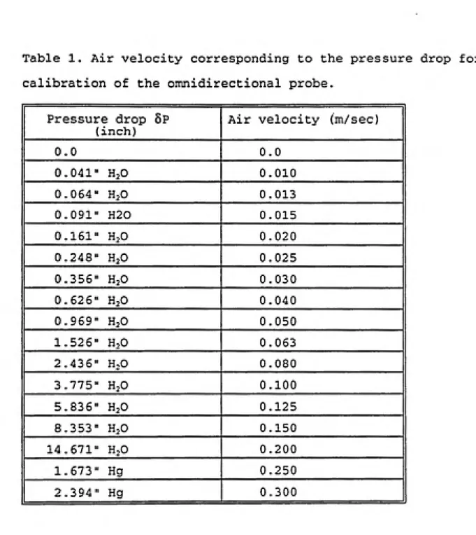
calibrated using data in Table 1.
3. Procedures for measuring air velocity
a) Connect the probe and the CTA system with the cable
of the calibrated length.
b) Turn on the computer, the CTA system, and the voltmeter.
c) Access the ACQwire program.
d) Load the calibration file. e) Activate the velocity channel.
f) Load the parameter file and calibration file. Select
sampling time and frequency.
g) Set the velocity range.
h) Measure air velocity with the "acquire raw data"
menu.
i) Input the current temperature (°C) of the
Table 1. Air velocity corresponding to the pressure drop for calibration of the omnidirectional probe.
Pressure drop 6P j (inch)
Air velocity (m/sec)
1 0.0
0.0 1
0.041" H2O 0.010 0.064" H2O 0.013
0.091" H20
0.015 1
0.161" H2O0.020 II
0.248" H2O 0.0250.356" H2O
0.030 II
0.62 6" H2O0.040 1
0.969" H2O0.050 1
1.52 6" H2O 0.0632.43 6" H2O
0.080 1
3.775" H2O 0.1005.83 6" H2O 0.125
8.3 53" H2O
0.150 II
14.671" H2O 0.2001.673" Hg
0.250 1
1 2.3 94" Hg
0.300 1
j) Convert the raw data (in voltage) to velocity after
the measurement is done.
k) List data or export data to a ASCII code file.
4. Measurement of air movement with a single probe a) Measurement in the nonventilated room.
The measurement of air movement in the nonventilated room
provides information to help explain why spatial variation
increases with an increase of distances between samplers. The
measurement was conducted with one probe located at the either
sites of B-B and C-C pairs of samplers (Figure 1). The
sampling frequency was 5 Hz/sec. The sampling interval was
102.4 seconds. The total number of samples for each set of
data was 512. Eight sets of data were collected at each
location. Measurement of air movement started ten minutes
after the probe was moved.
Five sets of data were collected to study the influence of
door opening on air movement at both locations. The door of
the nonventilated room was opened once for 3 0 seconds or five
times within 30 seconds while measurement was being conducted.
b). Measurement in room S-250.
The measurement was conducted with a single probe located
consecutively at the position of samplers A, B and C (Figure
3) . At each location, air velocity was measured at four
conditions of air movement: the heating ventilation and air conditioning system (HVAC) and the hoods on, the HVAC system on and the hoods off, the HVAC system off and the hoods on, and the HVAC system and the hoods off. Eight sets of data
were collected at each location for each air movement
condition.
5. Synchronization of collection of bioaerosols with measurement of air movement
In this experiment, bacteria were collected with two pairs of the Andersen two-stage samplers. Air movement was measured with two probes which collected data simultaneously. Two pair of samplers were located at the front of two hoods respectively. The distance between one pair of samplers and the face of one hood was 50 cm. Samplers were 80 cm off the floor (Figure 7) and each probe was immediately above and on the center line of each pair of samplers 30 cm (110 cm off
floor).
Bacterial samples were collected at four conditions of air movement: the HVAC system on and the hoods off, the HVAC
system and the hoods on, the HVAC system off and the hoods on,
or the HVAC system and the hoods off. For each condition of
air movement, two sampling runs were collected. Four
samplers were simultaneously operated to collect samples in
velocity was measured. If air velocities at both locations
had been approximately equal, samples could be collected and
air velocity would be measured during the sampling period.
The sampling time was ten minutes and the interval of
measurement of air velocity was 6.83 minutes. Air velocity
was usually measured ten minutes after the change in
conditions.
C. Data analysis
1. Non-parametric statistical methods
In the traditional statistical methods, data is usually
analyzed based on the assumption that the errors follov; the
normal distribution. Data may not be normally distributed so
analysis of data with a t test, or F test may not be accurate.
Use of small samples precludes the application of the central
limit theory.
Without an assumption of distribution, non-parametric
statistical methods may be adequate to analyze data with small
sample sizes. The non-parametric methods have been
recommended for analysis of bioaerosol data (H.A. Burge and
W.R. Solomon, 1987). Nonparamettric methods are usually less
powerful than parametric methods, assuming that the
distribution of the errors is known.
The sign test is one of the simple nonparametric tests for
paired samples. This method is useful for the analysis of
data in this study, such as samples collected with the A-A
pair of samplers (Figure 1) in the nonventilated room. By
comparing concentrations of samples collected with the Aj
sampler with those of samples collected with the Bi sampler
(the A-A pair of samplers contains of A and B samplers), the
number of sample concentrations at location A greater than
those at location B belongs to a binomial distribution under
the null hypothesis. The probability that the number of
sample concentrations collected at location A are greater than
those collected at location B can be computed by the chance,
0.5, for Al > Bl or Bl > Al. This method is used to determine if concentration of samples collected at location A is equal
to those collected at location B. The null hypothesis is
concentrations of samples collected at location A equal
concentrations of samples collected at B. The analysis is
tested at alpha level of 0.05. The test is based on
P{X > x} > 0.025 and P{X < 10 - x} > 0.025 (eq. 2-7) .
X is the random variable, and x is the number of sample
concentrations collected at location A greater that those
collected at location B. An example will be given in the next
chapter.
2. Analysis based on log-normal distribution
Most pollutant concentrations appear to belong to a
normal distribution (N.A. Esmen and Y.Y. Hammad, 1977) . Data was transformed by taking logarithms and was then analyzed with the t test, multivariable regression or variance component analysis. Regression analysis was used to find the relationship between the concentration of samples and independent variables: temperature, relative humidity, and wind speed. The applicability of transformation will be diagnosed by plotting residues v.s. predicted values.
3. Spatial statistics
The crucial parameter in geostatistics is the semivariogram, based on the secondary stationary assumption (B. Preat, 1987). The assumption is that the mean and the variance of concentrations of bioaerosols are constant in an
environment and the covariance is independent of the sampling site but dependent on the distance between sampling sites. The semivariogram value was computed by the equation,
SW = (I (C^i-Cbi)2)/n (eq. 2-8).
and i = 1, 2 .., n. Cj, and C^ were bioaerosol concentrations collected at location A and location B respectively. The
semivariogram may be thought of as an average variance. If
data belong to the normal distribution, the unbiased estimator
for variance, 5^, is
'^WJW
s^ = Z (Xi -x*)V(N-l) (eg. 2-9).
where x* = Lx^/N, and N is the number of samples. If N = 2,
and Xi = Ca and Cj,, the estimated variance
= tC, -(C. + Cb)/2]2 + [Cb - (C3 + Cb)/2]2
= (C^ - Cb)V2 (eq. 2-10),
which looks like semivariogram. The average of (Cg -C^)^ could
be thought of as the unbiased estimator for variance, so
semivariogram could be an indicator of spatial variation.
The relative semivariogram is computed to eliminate the
influence of the mean concentration of a pair of samples on
the semivariogram values. The relative semivariogram value is
defined by the following:
RSW = [2 ((C3i-Cti)/(C,i+Cbi))']/n (eq. 2-11).
and i = 1, 2, ...., n. The formula is very similar to the
coefficient of variation. Coefficient of variation is defined
as o/|i and usually estimated with s/x*. The square of
coefficient of variation is (s/x*)^. If x^ = C^ and C^,
(s/x*)2 = ^
{[C, -{C3 + Cb)/2]2 +[(Ct - (C, + Cb)/2]2} * [(C, + CJ/2]-2
= 2*[(Ca - Cb)/(C3 +Cb)]' (eq. 2-12).
The relative semivariogram was computed for samples collected
on different days. The mean bioaerosol concentrations were
highly variable over time. The relative semivariogram values
can be used as an index to compare spatial variation of
sampling bioaerosols on different days. The semivariogram or
relative semivariogram values present spatial variation adequately since the t test and the sign test do not reject
equal concentrations collected by two samplers so that
concentrations can be assumed equal.
4. Temporal variation
Autocorrelation coefficients were computed as indicators of temporal variation, by using the equation,
r(h) = C(t)*C(t+h)/Var(C) (eq. 2-13). C(t) is bacterial concentration collected at time t, C(t+h) is bacterial concentration collected at t+h, Var(C) is variance
of bacterial concentration for a particular data set, and r(h)
is the r*"^ order autocorrelation coefficient for this
particular data set. r(h) indicates that bacterial
concentration collected at time t+h depends on bacterial
concentration collected at time t.
Other methods are used to present temporal variation for
a particular data set. Variance component analysis directly
estimates and tests the significance of temporal variation.
The alternative is plotting bacterial concentration with time
on a particular day. The plotting method was used by Yeh H.c.
to compute an autocorrelation coefficient or when autocorrelation coefficient is not significant, plotting
bacterial concentrations with time presents temporal variation
clearly.
IV.RESULTS
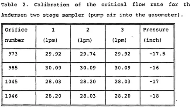
A. Calibration of the Andersen two stage samplers Table 2 shows the results of Andersen two-stage calibration. Results indicates critical flow rate varies with orifice nuii±)er. Based on the critical flow rates, these four samplers may be classified into two groups. Group 1, the orifice number starting at 900, has a critical flow rate of 30 1pm, and group 2, the orifice number starting at 1000, has a
critical flow rate of 28 1pm.
Only the 973 orifice, however, has a fl6w rate of 28 1pm
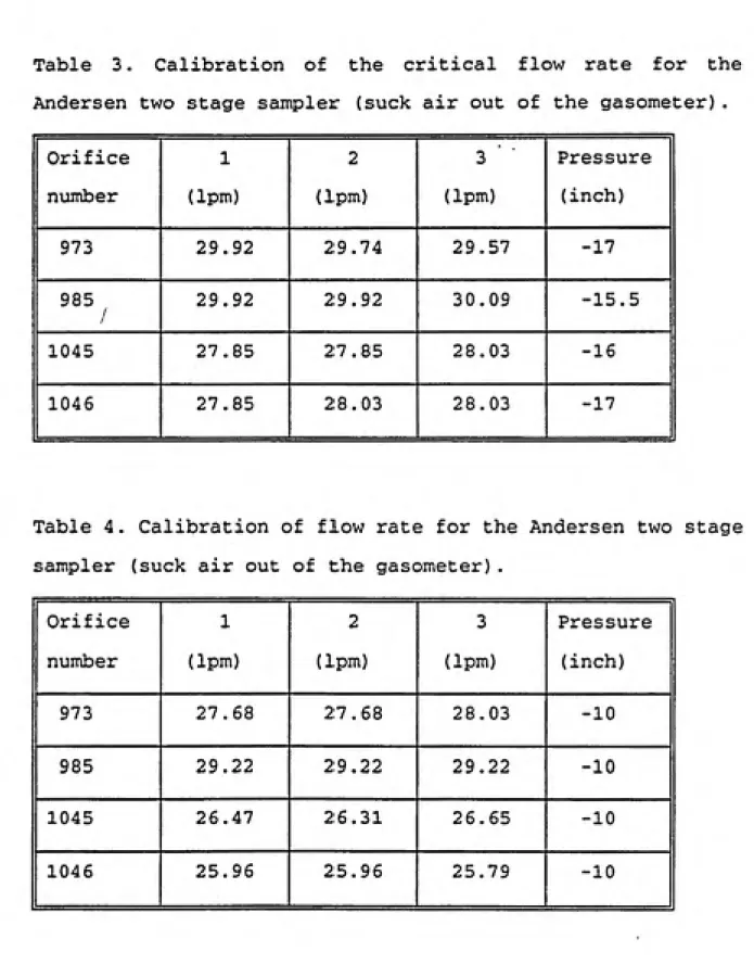
at a vacuum pressure of 10 inches Hg. The 985 orifice has flow rate higher than 28 1pm at a vacuum pressure of 10 inches Hg. Both 1045 and 1046 orifices have flow rate less than 28 1pm at a vacuum pressure of 10 inches Hg (Table 3. and 4.).
B. Comparison of the intra-paired variation
Although the critical sampling flow rates of the group 1 samplers (973 and 985) are higher than those of group 2 samplers (1045 and 1046), results show that sampling bacteria with the sampler (985) does not cause additional variability, compared with the samples collected with the group 2 samplers.
Semivariogram values can be compared to evaluate relative
variability.
Table 2. Calibration of the critical flow rate for the Andersen two stage sampler (pump air into the gasometer).
Orifice number
1 (Ipm)
2
(Ipm)
3 (Ipm)
Pressure
(inch)
1 973
29.92 29.74 29.92-17.5 II
1 985
30.09 30.09 30.09-16 1
1 1045
28.03 28.20 28.03-17 1
Table 3. Calibration of the critical flow rate for the
Andersen two stage sampler (suck air out of the gasometer).
Orifice
number
1 (Ipm)
2 (1pm)
3 ͣ
(1pm)
Pressure
(inch)
973 29.92 29.74 29.57 -17
985 /
29.92 29.92 30.09 -15.5
1045 27.85 27.85 28.03 -16
1046 27.85 28.03 28.03 -17
Table 4. Calibration of flow rate for the Andersen two stage sampler (suck air out of the gasometer).
Orifice
number
1
(Ipm)
2 (Ipm)
3 (Ipm)
Pressure
(inch)
973 27.68 27.68 28.03 -10
985 29.22 29.22 29.22 -10
1045 26.47 26.31 26.65 -10
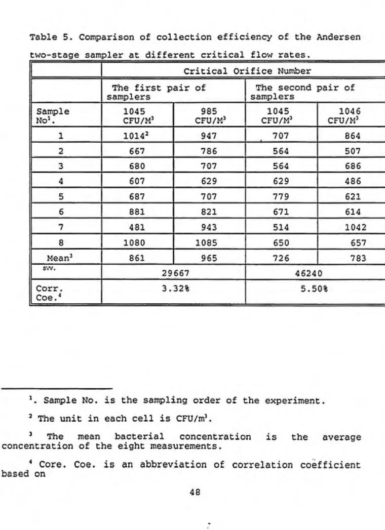
Table 5. Comparison of collection efficiency of the Andersen two-stage sampler at different critical flow rates.
Critical Orifice Number The first pair of
samplers
The second pair of samplers Sample No^ 1045 CFU/M^ 985 CFU/M^ 1045 CFU/M' 1046 CFU/M'
1 1014^ 947 707 864
2 667 786 564 507
3 680 707 564 686
4 607 629 629 486
5 687 707 779 621
6 881 821 671 614
7 481 943 514 1042
8 1080 1085 650 657
Mean^ 861 965 726 783
S'A'.
29667 46240
Corr.
Coe."
3.32% 5.50%
^. Sample No. is the sampling order of the experiment.
^ The unit in each cell is CFU/m\
^ The mean bacterial concentration is the average
concentration of the eight measurements.
The semivariogram value of the first pair of samplers (985 and 1045) is lower than that of the second pair of samplers
(Table 5.). The correlation coefficient of the first pair of samplers is also lower than that for the second pair of
samplers,
C. Temporal and spatial variation for the total counts.
1. Samples collected in the stairwell
A total of 30 runs of samples were collected at each
distance between samplers (Fig.l). Data is first analyzed with the sign test. Then, the semivariogram values or the relative semivariogram values are computed.
Data in Table 6 shows bacterial concentrations collected
with two Andersen two-stage microbial samplers located
adjacent on a particular day in the nonventilated environment. The collected bacterial concentrations are highly variable in
this environment. This highly variable data is analyzed with
the sign test. The null hypothesis asserts that mean bacterial concentrations collected with sampler A equal those of sampler B.
Hq: Ca = Cb (or Cb/C, -1 = 0)
Hi: C3 > Cb (or d, > C^)
With the t test, the statistics is T, and
T = N°-^*(u-H)/s. (eq. 3-1) .
N is the sample size and is equal to 10. u is the mean of
(Ca/Cb - 1) and is equal to -0.0906. |i is the true mean of (Ca/Ct, - 1) and is equal to 0 given C^ = C^. s is the standard deviation of (Ca/Cb - 1) and is equal to 0.1475.
T = 10°-^*(-0.0906-0)/0.1475 = -1.942. (eq. 3-2). According to a two-tail test, Pr{ T < -1.942 or T > 1.945} >
0.05. Ho cannot be rejected at the 0.05 level. Therefore, the
null hypothesis is accepted. Bacterial concentrations
collected with sampler A are equal to those collected with
sampler B.
with the distribution-free sign test, the sign number is
1 if Cfc Ca > 0. The sign number is 0 if Cb Ca < 0. If C^ -Cb = 0, the data is discarded. The sum of the sign numbers
is the statistics of the distribution-free test. For the
sample size of 10, the critical number is 2 at 0.05 level.
Since the statistics of these data in Table 6 is 3 > 2, Hq
cannot be rejected at 0.05 level. The null hypothesis is also
accepted. The distribution-free test also shows
Table 6. The Example for the t test and distribution-free
sign test^.
1 Sample
No.
A <C,)
CFU/M'
B (CJ
CFU/M^ 1
Sign
II 1
250 264 0.0561 II
2 321 286 -0.109
0 1
1 ^
500 307 -0.3860 1
II ^
300 264 -0.120 1
1 ^
471 414 -0.1210 II
1 ^
343 300 -0.125 07 343 271 -0.21
0 1
1 ^
193 221 0.145 11 ^
364 343 -0.0580 1
1
ͣ
^^
314 321 0.022 1SUM -0.906 3^
^. Samples were simultaneously collected with two samplers
located side by side.
*. The sum of the sign numbers for the set of data is the
statistics for the distribution-free sign test.
that the bacterial concentrations collected with sampler A are equal to those collected with sampler B. In fact, the distribution-free sign test is based on binomial distribution. If samples were collected randomly, the probability that C^ > Cb or Cfc > C, would be 0.5. On the other hand, the probability that the sign number is 1 or 0 is 0.5. The sum of the sign numbers is the statistics, the number of data in which Ct, > C^. If the sum of the sign number is x, the probability that x is
equal to n will be
Pr{ X = n, n <= 10 }
= 10!/[(n!)*(10-n) !] *(0.5)'^*(0.5)^°-"
= 10!/[ (n!)*(10-n) !] * (0.5)^°. (eq. 3-3). Since the statistics of this set of data is 3, the
distribution-free sign test is based on
Pr{x<=3 } =Pr{x=0 } +Pr{x=l } + Pr{ X = 2 } + Pr { X = 3 } > 0.05,
and Pr{ x >= 7 } > 0.05.
Since Pr{ x < = 3 } +Pr{ x >= 7 } > 0.05, the distribution-free sign test also show that the null hypothesis can not be
rejected at 0.05 level.
Based on the t test and the distribution-free sign test, the bacterial concentrations were equal when collected by two Andersen microbial two-stage samplers located adjacent in the
between bacterial concentrations collected with two adjacent
samplers.
The test and the distribution-free sign test are also used to analyze samples collected with two samplers located a distance of 50 cm, 100 cm, and 470 cm, and results also shov;
that there is no difference of bacterial concentrations.
Table 7. The comparison of spatial variation of samples
collected at different distances between two samplers with semivariogram and relative semivariogram values.
Distance between two samplers (cm) The mean cone, collected at location A The mean cone, collected at location B Semi¬ variogram values Relative Semi¬ variogram values
1 °
243 220 27370.0089 II
1 ^°
76 75 321 0.017461 100
79 73 5660.02264 1
j 47 0
122 118 1158 0.02881Semivariogram values = sum of all (Ca-Cj^)^ / number of
samples collected at a particular distance.
1. Relative semivariogram values = sum of all { (C„-Cj^) / (C^+Ct) )^
divided by number of samples collected at a particular
distance.