thesis_hptaylor.pdf

(1)

Normal Modes of the Structural

Connectome

Exploring the harmonic modes of the human brain using a graph

model of its geometry

Hoyt Patrick Taylor IV

Undergraduate Honors Thesis

Physics

(2)

Acknowledgements

This project would not have been possible without the generous support of the many wonderful people that helped me throughout the 2018-2019 academic year. I offer my deepest and most sincere gratitude to: Dr.

Bert Dempsey, a neighbor and long-time family friend, who took the time to read an early (and therefor confusing!) draft of this manuscript and offered helpful feedback; Ye Wu, who helped me learn how to use the MRtrix3 software package and generated tractograms of 20 million fibers for 10 subjects (which are not

used in the results shown here, but will hopefully be used in continuation of this work); Dr. Zhengwang Wu, who was incredibly kind and unfailingly generous with his time, and helped me with a myriad of different technical obstacles throughout the course of this project; my adviser Dr. Rosa Tamara Branca, who enabled me to conduct this research for the Physics department, kept me honest about both my time

management and the physical interpretation of the model presented here, and who provided invaluable feedback on drafts of this manuscript; my advisers Dr. Han Zhang and Dr. Pew-Thian Yap, who met with

me for a minimum of 1 hour every week over the course of this project and responded to dozens (hundreds?) of rambling emails, providing technical guidance without which this work could not exist; my parents Katie and Hoyt Taylor, who provided much-needed moral support throughout this project, and to whom I owe both the countless opportunities that put me in the position to begin this work and my very existence; and the many other individuals not explicitly named that helped me in various ways during the

(3)

1 Introduction

1.1 Modelling

When attempting to enumerate a theoretical framework governing the dynamics of complex systems, it is advantageous to simplify the system of interest. Although the potential experienced by an electron orbiting a proton is not solely described by the Coulomb interaction between the opposing charges, the wavefunctions and associated energies obtained by solving the Schrodinger equation with this simplified Hamiltonian of the Hydrogen atom are quite close to those obtained using degenerate perturbation theory and the full Hamiltonian. The human brain contains over 100 billion neurons, with on the order of 73 connections per neuron [1]. Aside from the reality that current empirical methods are not capable of accurately measuring the geometry of these connections at all scales of detail, the sheer geometric and cytoarchitectural complexity of this structure represent massive obstacles to bottom-up inference of the guiding principles of brain dynamics. While individual neurons are capable of complex information processing, and their properties still con-stitute an active and open area of research, it has been proposed that on the population level, their behavior resembles that of tiny springs [2]. The model presented here draws on this simplification. We postulate that this simplification is akin to the simplification of the Hamiltonian of an electron in a Hydrogen atom to only its Coulomb interaction with the nucleus.

A proverbial tenant of biology states that the structure of biological systems underlies their function; function is solely explained by structure. In simple small-scale biological systems, this has been increasingly validated [3, 4, 5, 6]. There is more difficulty, however, in establishing this link in the human brain. While there has been moderate success of studies seeking to identify correlation between the structure of the brain and its temporal-spatial patterns of activation as measured by functional magnetic resonance imaging (fMRI), there are relatively few successful attempts to predict function from structure [7, 8, 9, 10].

This work describes a simple, fully data-driven model and processing pipeline that, from structural brain images, yields a complete, orthonormal basis of spatial patterns of functional activity on the human cortex. These patterns are referred to as structural connectome normal modes, harmonics, and eigenvectors. By virtue of its completeness and orthonormality, the basis of structural connectome normal modes is capable of describing any pattern of functional activation on the surface of the human brain quantified at or below the spatial resolution of the eigenfunctions. Further, we demonstrate that the information contained in a very small fraction of this basis can be used to calculate neuroanatomically meaningful parcellations of the cortex on the subject and group level at varying resolutions, and that calculated parcellations agree well with those in the literature derived from a wide array of brain features, including functional connectivity.

1.2 Laplacian Eigenfunctions

(6)

the general wave equation, and many other successful descriptions of physical phenomena. Many currently accepted explanations of complex physical systems owe their existence to the suitable formulation of a differential equation involving the Laplacian operator. Perhaps the most glaring example of this is the Schrodinger equation, which accurately predicts phenomena that were mystifying to the scientific community prior to its existence, and which is capable of describing dynamics of systems with infinite dimension.

The eigenfunctions of the Laplacian operator imposed on a flat, one-dimensional domain form the extraor-dinarily powerful Fourier basis, through which many of the most physically relevant dynamical paradigms can be described. The Fourier basis is universally used in analysis of countless physical systems that can be parameterized by one variable. Similarly, the orthonormal bases yielded by eigendecomposition of the Laplacian imposed on more complex domains are in many instances particularly convenient for representing physical dynamics parameterized by that domain [11, 12]. For instance: the steady-state modes of vibration of an elastic membrane held still at its edge by a rigid circle are the Bessel functions- the eigenfunctions of the Laplacian imposed on a circular, bounded domain. This basis can be used to efficiently represent all of the possible dynamics of the head of a drum. Here, a novel discrete model of a graph that parameterizes the structural geometry of the human cortex is presented, the eigenvectors of the Laplacian imposed on that domain are graph are calculated, and the efficacy of these normal modes as meaningful biological patterns is tested and verified. It is important to note that this model is largely based on that used by Atasoy et. al [13], however several important differences in the present model including the density of sampling of structural connectivity, the method of tractography used, the weighting of elements of the graph, and the implementation of multi-layer graph methods all render this model distinct and more robust. Additionally, the use of eigenvectors of the laplacian matrix of this graph model to parcellate the cortex into distinct functional regions is entirely novel.

1.3 Cortical Parcellation

Cortical parcellation refers to the division of the human cortex into distinct functional regions. This is important as neuroscience seeks to associate human behaviors and psychiatric pathologies with specific brain regions. The first and most extensively referenced parcellation scheme was devised by Korbinian Brodmann, and was based on a post-mortem examination of the cytoarchitecture of the brain. Research since then has revealed that in many instances, the layout of cell types in the brain does not always directly correspond to the layout of functional regions. Further, it is becoming increasingly clear that the organization of the brain is is hierarchical; for any given region, there exist multiple sub-regions with distinct function. Based on this, it is obvious that there might be no ground-truth division of the cortex, as there are a functionally unlimited number of resolutions at which the brain can be parcellated. For this reason, it is difficult to establish a consensus in the community on the best method of parcellation.

(7)

distinct lobes [14]. This result shows that the vibrational modes of a membrane shaped like the surface of the cortex are predictive of its large scale functional organization. Many previous studies have used measures of long-range white matter connections to parcellate the cortex [15, 16, 17]. Although several of these have achieved agreement with existing functional and histological measurements, to the author’s knowledge, all previous work has relied on coarsely discretizing the cortex using prior anatomical information. In contrast, this work does not employ any neuroanatomical priors, and discretizes the cortex and its long-range structural connectivity at an unprecedented level of detail, resulting in unbiased, potentially more accurate, and more detailed parcellations.

2 Methods

2.1 Data and Preprocessing

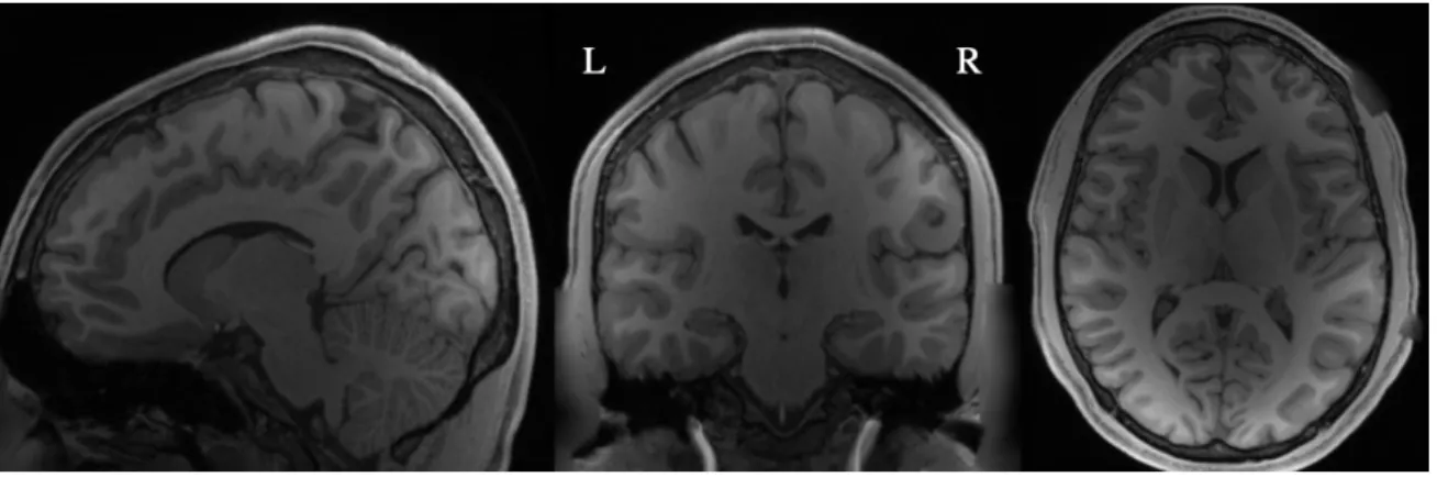
Anatomical or T1-weighted MRI scans provide high contrast between the brain’s white matter- the regions of the brain comprised of long-range neuronal axon fibers- and the brain’s gray matter- the tissue comprising the cortex (the outer layer involved in all high-level cognitive processes) containing a high density of neuronal cell bodies. The white matter/ gray matter interface refers to the region separating these two types of tissue.

Figure 1: Example T1-weighted anatomical MR image for subject 1 from different view angles.

(8)

2.2 Computation

All computations were performed locally on a laptop computer with a 6 core Intel i9 3.5 GHz processor and 32GB of RAM. As the computational scope of this work is quite broad, in instances in which existing open-source software packages were capable of achieving the computational processes or set of processes efficiently, these packages were downloaded and used.

2.2.1 MRtrix

All algorithms used in the processing of diffusion weighted MRI images to produce tractograms of 2.8 million fibers per subject (described in 2.3) are included in the open-source MRtrix3 software package, which is extensively documented athttps://mrtrix.readthedocs.io/en/latest/index.html. [20, 21, 22].

2.2.2 MATLAB+Paraview

All visualization was performed using ParaView [23]. Interfacing between Python and ParaView was achieved by first writing relevant arrays from Python to text files, and then writing ParaView-compatible files using the text files and an open-source MATLAB-wrapped package calledmvtk.

2.2.3 SciPy

The matrices constructed in this work are too large to be stored and manipulated using standard numerical data structures on the local machine with 32GB of RAM. The matrices are in general sparse, and therefor special data structures designed for dealing with sparse matrices allowed for efficient manipulation. Specifi-cally, methods within thescipy.sparsesub-library of SciPy- an open-source scientific programming library included in most downloads of Python3- was used to construct, manipulate, and solve for the eigenvectors and eigenvalues of the matrices [24].

Additionally, the calculation of dice score detailed in 5.1was performed using the dice method of the

scipy.distancesub-library within SciPy.

2.2.4 SciKit-Learn

For the matching of the 2.8 million endpoint coordinates to their nearest neighboring of the 81,924 white matter surface vertices (described in3.1.2) and for the matching of white matter surface vertices lying on the mid-brain structures to their nearest neighboring vertex on the opposite hemisphere (described in3.1.1), an efficient nearest-neighbors algorithm was necessary. Of the several different open-source algorithms tested, the most efficient was determined to be theNearestNeighborsmethod from theneighborssub-library of SciKit-Learn open-source Python3 library [25].

(9)

sub-library. Additionally, the normalized mutual information score (described in5.1) was calculated using the

normalized mutual info scoremethod of themetricssub-library of SciKit-Learn.

2.2.5 NumPy

All other data manipulations not explicitly mentioned in2.2.1-2.2.4 were either performed directly using methods available within the NumPy python library, or performed using Python functions heavily relying on NumPy methods written by the author as detailed below.

Functions used in the construction of matrices and eigendecomposition thereof are contained in a script calledspectral graph.py. Functions used in the analysis of the vector spaces described by individual sets of eigenvectors (described in4.1) are contained in a script called SubjectAnalysis.py. Functions used to perform spectral clustering are contained in a script calledClustering.py. Functions used to construct the super-adjacency matrices described in4.3and to perform numerical analysis of the consistency of parcellation results described in5.1are contained in a script calledClusterProcesses.py. Any and all of these scripts are available upon request to the author. Any data manipulations not performed with functions included in these scripts were performed in the iPython console and therefor are not explicitly documented, but attempted descriptions by the author are available upon request.

2.3 Diffusion Tractography

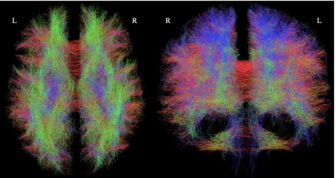
The diffusion MRI scans used provide a measure of the diffusivity of water in 60 different directions at every voxel (cube of side length 1.25mm) in the brain. Water diffuses more easily in the direction of white matter axonal fiber bundles. Diffusion tractography seeks to estimate the orientation of white matter fibers based on the diffusion magnetic resonance signal.

From the multi-shell, high resolution, registered diffusion MRI scans of each subject, the b=1000 mm_s2

(10)

Figure 2: Example tractogram of subject 1 with 100,000 tracks. A lower number of tracks are shown for visualization purposes, as individual fibers are not visible in the tractograms of 2.8 million fibers. Fibers are colored according to direction.

2.4 White Matter Surfaces

(11)

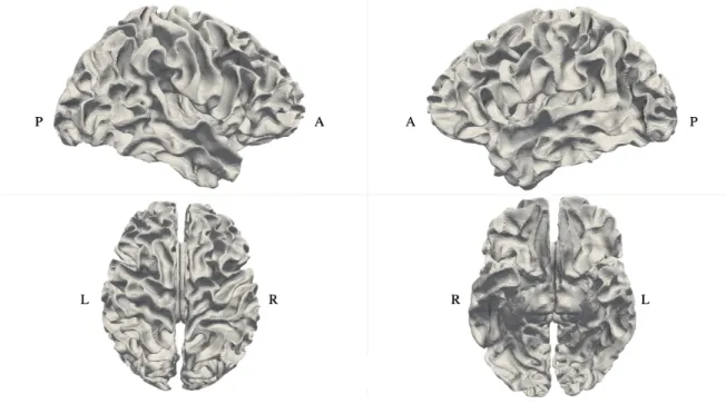
Figure 3: Resampled and registered white matter surface mesh of subject 1 from different view angles. ”L” and ”R” refer to left and right. ”A” and ”P” refer to anterior (front) and posterior (back).

The spatial coordinates of the vertices and the connections defining the polygonal mesh were extracted and stored for each subject. For a given subject, these vertices are given by

V ={vi|i∈0..1...Nvert},

vi= (xi, yi, zi)

(1)

where Nvert=82,924.

3 Graph Formulation of Structural Connectome

3.1 Graphs

A graphGis defined by a collection of vertices V and the edgesE between those vertices, given by

E={eij|(vi, vj)∈(V ×V)}. (2)

Although the vertices V may be embedded space in a particular way, the connectivity of G and all of its topological properties can be described by its adjacency matrix ˆA, which is populated by

ˆ

Ai,j= ˆAj,i=

    

wi,jif (i, j)∈E

(12)

(3)

where wi,j is the weight of the connection between vertices iandj.

Importantly, it has been shown that for a graph whose vertices are a sampling of a Riemannian manifold, in the limit ofNvert→ ∞, many of the properties of that graph approach their continuous analogs [26].

3.1.1 Surface Adjacency Matrix

By benefit of the vertex-vertex correspondence of the white matter surfaces achieved by the process described in 2.5, the indices of connected vertices are identical for all subjects, although the spatial embedding of vertices is variable. As graphs and their adjacency matrices are invariant to the spatial embedding of their vertices, only one adjacency matrix ˆAmesh is necessary to represent the surface mesh of all subjects.

For the surface mesh with Nvert, its adjacency matrix ˆAmeshis of size (Nvert×Nvert). Here, the spatial

resolution ofNvert=81,924 represents an unprecedented level of resolution for studies seeking to construct

graph models of the structural connectivity of the cortex. ˆAmeshis populated according to equation 3, where

the edges are between vertices connected by the polygonal connections that define the mesh, and the edge weightsws_i,j are all equal to 1.

It is important to note that ˆAmesh describes both hemispheres of the brain and as a result, there are two

fully-connected regions (the left and right hemisphere) ofG( ˆAmesh). This is a result of the fact that current

standard methods of constructing cortical surfaces from T1 weighted MR images- including those used to construct the surfaces used in this analysis- are only equipped to do so on a per hemisphere basis. When the two hemispheres are represented in a single graph, there exists a physiologically erroneous disconnection between them.

In order to correct for the fictitious division between the two hemispheres, an inter-hemisphere connection adjacency matrix ˆAIC was constructed by connecting all vertices lying on the midline structures (Corpus

callosum, brain stem, thalamus, etc) of the surface of each hemisphere to their nearest neighboring vertex on the opposite hemisphere with edge weightw_i,jIC=1. The full surface adjacency matrix ˆAswas then calculated

as Âs= Âmesh+ ÂIC.

The inclusion of ˆAICimproved both the left-right symmetry of structural connectome normal modes and

the symmetry of resulting parcellations. It is important to note that the construction and inclusion of ˆAICis

(13)

3.1.2 Long-Range White Matter Fiber Adjacency Matrix

All long-range white matter connectivity information relevant to this model is encapsulated by the spatial coordinates of the endpoints of each fiber and indices of endpoints that belong to the same fiber. Although the seeding and termination of tracts was constrained to the white matter/gray matter interface, the location of seeds was randomly sampled from a continuous domain representing this interface. Therefore, fiber endpoints are not in general at the precise location of the white matter surface mesh vertices.

In order to encode the connectivity information contained by the fiber endpoints in the space parameter-ized by the white matter surface mesh , each endpoint was associated with its nearest neighboring surface mesh vertex using SciLearn’s kd-tree nearest neighbors algorithm, where Euclidean distance was the metric. The average distance between fiber endpoints and their identified nearest neighboring surface vertex is less than the average spacing of surface vertices, indicating an effective matching.

The white matter fiber adjacency matrix ˆAm

f for each subject is formed identically to ˆAmesh, except that

its edgeswf_i,j correspond to white matter surface vertices connected by long-range white matter fibers, and is equal to 0.1. The lower magnitude ofwf_i,jwas determined through exploratory analysis of several different weighting strategies. This weighting strategy was determined to give the most physiologically meaningful representation of structural connectivity.

3.1.3 Total Adjacency Matrix

The number of nonzero elements of ˆAm

f , ˆAmesh, and ˆAIC are 2,860,971 (group-average), 491,520, and 9,636

respectively. The structural connectome graph proposed is described by its adjacency matrix ˆAm_{. For}

subjectm, ˆAm _{is given by}

ˆ

Am= Âm_mesh+ ÂIC+ Âf. (4)

It is worth noting that certain elements ofG( Âm) have weight 1.1 due to its definition as a sum of matrices, however it is overwhelmingly the case that the edges defined by Âm_f are not between the same vertices as those defined by Âmesh and ÂIC, and vice versa. This is shown by the fact that the number of nonzero

elements in ˆAm_{is approximately 3.22 million, whereas the sum of nonzero elements in each of ˆ}_Am

f , ˆAmesh,

and ˆAIC is approximately 3.36 million.

4 Normal Modes of the Structural Connectome

The Laplacian matrix ˆLof graphG( ˆA) is defined as ˆ

L( ˆG) = ˆD1/2AˆDˆ1/2, (5)

where

ˆ

Di,i= Nvert

X

j=0

(14)

As stated in 3.1, in the continuous limit of graph representations of manifolds, the Laplacian matrix approaches the continuous Laplace-Beltrami operator. This implies that, given a graph formed by a dense sampling of a manifold, the eigenvectors of the Laplacian matrix of that graph give the steady state vi-brational modes of that manifold [11, 27]. That is, the eigenvectors correspond to the spatial patterns of motion and the eigenvalues correspond to the energy or frequency associated with those patterns. Here, large

Nvertgives a good approximation of the continuous Laplacian. Further, the number of fiber connections (2.8

million) gives a dense sampling of structural connectivity in comparison with the only other study seeking to calculate connectome harmonics [13].

The physical interpretation of the eigenvectors of this graph is somewhat ambiguous; although the present model seeks to parameterize the human brain, which is continuous, our graph model could also describe a collection of masses connected in a network by springs. N masses connected by a network of springs with effective spring constantsks

i,jbetween massesiandjcan be represented by a graph whose adjacency matrix

ˆ

Aspringis populated according to equation 3, where the edge weights areksi,j. The normal modes of vibration

of the physical system described by ˆAspringare the eigenvectorsψkof the laplacian matrix ˆL( ˆAspring), given

by

ˆ

Lψk=λkψk. (7)

Notably, this formulation is identical to the present formation of the structural connectivity graph, where the ‘ effective spring constants’ are 1 for vertices connected by the surface mesh, and .1 for vertices connected by long range fiber connections. We set up these parameters in light of the assumption that local coupling of the cortex (through short fibers and other short-range connections) is stronger than coupling due to long range fibers (association, projection and commissural fibers). The high level of heterogeneity in whole brain functional connectivity profiles under various task regimes gives evidence that this assumption is valid. In parallel, the high proportion of edges defined by fiber connections implies that much of the geometric complexity of the human brain is contained in its white matter geometry, which is trivially obvious.

4.1 Individual

Nharm structural connectome normal modes, ψ0. . . ψk. . . ψNharm and λ1 < λ2 < . . . < λNharm, for each subjectmwere calculated according to equation 7, with ˆL=L( ˆAm_{) .}

Here, Nharm=99. ψ0 is the trivial solution to the eigen-problem, contains no meaningful information, and is thus excluded from the set of eigenvectors. Several exploratory analyses of the relationship between the eigenvectors of different subjects were conducted. Each subject’s set of eigenvectors is self orthogonal:

{i6=j|0...Nharm},

hψi, ψji= 0,

(8)

(15)

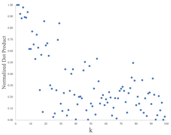
populated according to a different set of 2.8 million long range white matter connections, there is no guarantee that the subspaces described by each subject’s calculated set of eigenvectors are equivalent. Visual inspection of the eigenvectors of different subjects color mapped onto the white matter surface reveals that similarity between across subjects degrades for wavenumberk >10 . Figure 4 demonstrates this by the decay in the normalized dot product between corresponding eigenvectors for a pair of subjects.

Figure 4: Normalized dot product of corresponding eigenvectors of subjects 1 and 3

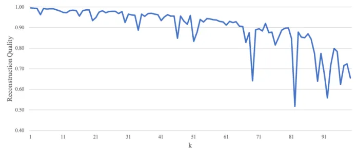
In order to investigate the similarity of the subspaces represented by each subject’s eigenvectors, we define subjectn’s reconstruction quality Ωn,m_k of eigenvectorkof subjectm as:

Ωn,m_k =hωkn, ψkmi, (9)

where

ω_kn,m=

Nharm X

j=1

(16)

Figure 5: Overlap of subspaces. Ω3_k,1 is plotted versus k. The reconstruction quality is high throughout the spectrum, with few individual exceptions and a slight decay neark= 85. This indicates a high degree of overlap between the subspace represented by subject 3’s eigenvectors with the subspace of subject 1’s eigenvectors.

4.2 Group Average

In addition to calculating connectome harmonics from each subject’s ˆL(Am),Nharmgroup average harmonics,

ψk ,were calculated fromL=L(A), where

A= 1

Nsub Nsub

X

m=1 ˆ

Am, (11)

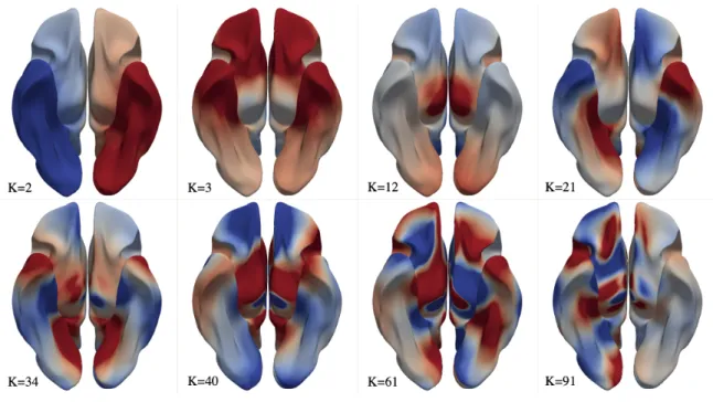
where in this study, the number of subjectsNsub = 10. Figures 6 and 7 display selected average

(17)

Figure 6: Selected group-average connectome harmonics viewed in −z direction. Red indicates positive values and blue indicates negative values.

(18)

4.3 Multi-Layer Graph

GivenM graphsG(Am_{), each with N vertices, a multi-layer graph can be represented by the super-adjacency}

matrixA, a block-diagonal matrix whose diagonal blocks of size (N ×N) are the adjacency matricesAm_,

and all other blocks are the identity matrix multiplied by an inter-layer weighting strengthγ.

When the vertices of the subgraphsG(Am_{) represent the same features, and properties common to all M}

are of interest ,G(Am)provides useful information regarding both the common features and the differences between the set ofG(Am)’s [28]. Multi-layer approaches have been employed in many neuroimaging studies, including in the work of Lefevre et al [14], which uses spectral clustering of the eigenvectors of the laplacian matrix of a fully surface-based graph to coarsely parcellate the cortex into 5 major regions. These studies demonstrate the efficacy of multi-layer approaches to establish group-level correspondence between features of individuals while preserving individual differences [28, 14].

Here, a super adjacency matrix of size (819,240×819,240) was constructed using the individual adja-cency matrices Am_{. The eigenvectors of the super adjacency matrix} _A_, _ψ_{, are of length} _N

vert ×10. A

subject’s, individual multi-layer eigenvectors ˜ψm

k are defined as the lengthNvert sections ofψk with indices

correponding to those of that subject’s Am _within_A_{. In contrast to the individual eigenvectors, there is}

high similarity between ˜ψm_k acrossm. In subsequent analyses, the effect of varying the inter-layer weighting strengthγis explored. As expected, the magnitude ofγwas found to correspond to the degree of coherence of eigenvectors across subjects.

5 Clustering and Parcellation

As a test of the hypothesis that the eigenvectors of the Laplacian matrix of the present graph model of the structural connectomes reflect physiologically meaningful spatial patterns of the function of the human cortex, vertices of the white matter surface were hierarchically clustered by their ‘eigenprofile’, or spectral coordinates. We define the eigenprofile ofvi asxi, where

xi= [ψ1(vi), ψ2(vi), . . . , ψN harm(vi)]. (12)

Hierarchical clustering of vertices based on their spectral coordinates was performed using SciKit-Learn’s Agglomerative clustering algorithm. The matrix ˆAm

mesh+ ˆAIC was also inputted to the algorithm to speed

the tree construction initialization. The output of the algorithm when initialized with Nclust clusters is a

cluster label vector c of lengthNvert, with indices identical to the vertex indexing, and with an integer valued

entries (labels) between 0 andNclust indicating the cluster to which the vertex was assigned.

Clustering was carried out for each set of individual eigenvectors,ψm_{, for the group-average eigenvectors,}

(19)

5.1 Metrics of Variability

To measure the similarity between different clustering results, we employ two different metrics of similarity: the normalized mutual information score and the dice score. Mutual information between pairs of cluster label vectors was calculated as described in 2.2.4 with the two cluster label vectors as input. Dice score between two clusters was calculated by first binarizing the cluster labels, and calculating the dice score as described in2.2.3with the two binary cluster vectors as input. Both of these metrics take on a value between 0 and 1.

Dice score was used to investigate the distribution of similarity between pairs of clustering results across clusters, which is only meaningful when there is correspondence between the location of vertices given a particular label between the two clustering results being compared. Because the clustering algorithm was initialized independently for the clustering of individual eigenvectors, the resulting labels are not spatially coherent across subjects, and therefor the dice score was not used to evaluate their consistency.

5.2 Color Mapping

It is of interest to view parcellation results on the cortical surface in order to qualitatively compare them to existing parcellations in the literature. The scalar values representing cluster labels contained in given cluster label vectors are agnostic to the spatial distribution of the clusters on the cortex, as they are calculated solely from the spectral coordinates given by the set ofxi’s. Therefor, if the scalar values are directly mapped to

the white matter surface, each scalar value must be assigned a color through some method. For a relatively small number of clusters, it is not overly time-consuming to manually construct the color map (as is done in figure 8), however for largeNclust this method becomes implausible.

In order to efficiently assign cluster labels to a color based on spatial criteria, an python script called

ColorMap.py (available upon request to the author) that assigns each cluster label a unique red, green, blue (R,G,B) coordinate was written and employed for parcellation results whereNclust>80. ColorMap.py

(20)

5.3 Individual and Group-Average Parcellation

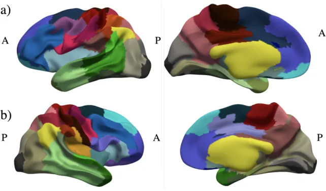
Figure 8: Parcellation result calculated usingψ’s withNclust= 80 manually color-mapped onto the a) left

(21)

Figure 9: Parcellation result calculated usingψ’s withNclust = 120 color-mapped using barycentric

coor-dinates onto manually color-mapped onto the a) left hemisphere and b) right hemisphere of the smoothed group average white matter surface. Parcel borders appear in black.

(22)

Figure 10: Mutual information between individual cluster label vectorscm_{and group-average cluster label}

vectorc.

As expected, the similarity between individual parcellations and the group average parcellations decreases with increasingNclust

5.4 Multi-Layer Parcellation

Clustering of the super eigenvectors gives a super cluster label vector c of length Nvert×10, and like the

multi-layer individual eigenvectors, the individual multi-layer cluster labels ˜cm _{are given by the length N}

(23)

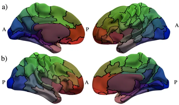
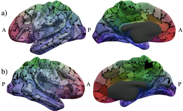
Figure 11: Consensus parcellation calculated using ˜ψ’s with Nclust = 500 andγ = 0.8 color-mapped using

barycentric coordinates onto the a) left hemisphere and b) right hemisphere of the smoothed group average white matter surface. Vertices for which all ˜cm _{do not agree are colored black.}

In contrast to individual cluster labelscm_{, there is spatial correspondence between cluster labels across}

m for the individual multi-layer clustering results ˜cm_{. To evaluate the effect of varying} _N

clust and γ on

the consistency of clusters both across subjects and across clusters, we first compute the consensus cluster labelling for a given set of individual multi-layer clustering results. The consensus labelling of a vertex is given a particular label only if the labels of that vertex agree across all subjects. Otherwise, it is given a label outside of the range of 0-Nclustdesignated as the disagreement label. Figure 12 demonstrate the effect

of inter-layer weightγand number of clusters on the cluster-wise agreement between individual multi-layer clustering results ˜cm_{and the consensus cluster labelling. As expected, agreement decreases with both}_γ_and

(24)

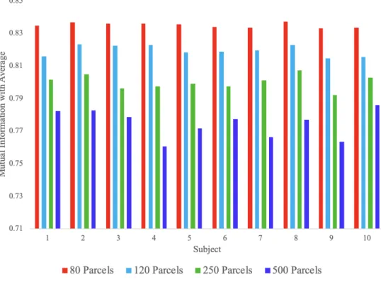
Figure 12: Mutual information with consensus parcellation for varying number of parcels and varying interlayer weighting strength.

(25)

Figure 13: Group average per-parcel dice score with consensus parcellation for a) 40 parcels with lowest average dice score from clustering with Nclust = 80 b) 250 parcels with lowest average dice score from

clustering withNclust = 500. Different values ofγ are plotted as separate lines, with the legend indicating

the color of the line and the value ofγ.

From figure 13, it can be seen that for high values ofγ, there is high similarity between all parcels and the consensus parcels, and that for lower values of γ, there are individual multi-layer clusters with little or no similarity to the consensus parcels of the same label. The number of these minimally-overlapping parcels increases with increasingNclust and with decreasingγ. This suggests that the value ofγ can be varied in

order to obtain a desired level of group-level correspondence of parcellations, and that the optimal value of

γ depends on the desiredNclust

5.5 Qualitative Comparison with Existing Parcellations

All calculated parcellations show qualitative similarity with various existing parcellations in the literature, including but not limited to those in [29, 30, 18]. This similarity is variable acrossNclust, which literature

parcellation is used as reference, and the particular clusters that show similarity. In general, higherNclust is

necessary to achieve similarity with literature between frontal-lobe parcels than for temporal, parietal, and occipital lobe parcels. Conversely, at highNclust, it is almost always possible to achieve similarity between

combinations of calculated parcels with larger parcels in literature parcellations.

(26)

normal modes that meaningfully reflect brain function.

Figure 14: Left hemisphere parcellation result calculated usingψ’s withNclust= 80 manually color-mapped

and labelled to resemble the MarsAtlas parcellation [30].

References

[1] Herculano-Houzel, S.: The human brain in numbers: a linearly scaled-up primate brain. Frontiers in Human Neuroscience (2009)

[2] Sardi, S., Vardi, R., Sheinin, A., Goldental, A., Kanter, I.: New Types of Experiments Reveal that a Neuron Functions as Multiple Independent Threshold Units. Scientific Reports (2017)

[3] Slack, J.M.: Molecular Biology of the Cell. In: Principles of Tissue Engineering: Fourth Edition. (2013)

[4] Saraste, M.: Biomembranes: Molecular structure and function. Trends in Biochemical Sciences (2003)

[5] Mercer, T.R., Mattick, J.S.: Structure and function of long noncoding RNAs in epigenetic regulation (2013)

[6] Lee, D., Redfern, O., Orengo, C.: Predicting protein function from sequence and structure (2007)

[7] Van Den Heuvel, M.P., Mandl, R.C., Kahn, R.S., Hulshoff Pol, H.E.: Functionally linked resting-state networks reflect the underlying structural connectivity architecture of the human brain. Human Brain Mapping (2009)

[8] Meuli, R., Honey, C.J., Sporns, O., Gigandet, X., Hagmann, P., Cammoun, L., Thiran, J.P.: Predicting human resting-state functional connectivity from structural connectivity. Proceedings of the National Academy of Sciences (2009)

(27)

[10] Damoiseaux, J.S., Greicius, M.D.: Greater than the sum of its parts: a review of studies combining structural connectivity and resting-state functional connectivity. Brain Structure and Function (2009)

[11] L´evy, B.: Laplace-beltrami eigenfunctions towards an algorithm that ”understands” geometry. In: Proceedings - IEEE International Conference on Shape Modeling and Applications 2006, SMI 2006. (2006)

[12] Niethammer, M., Reuter, M., Wolter, F.E., Bouix, S., Peinecke, N., Ko, M.S., Shenton, M.: Global Medical Shape Analysis using the Laplace-Beltrami-Spectrum. In: MICCAI07, 10th International Con-verence on Medical Image Computing and Computer Assisted Intervention. (2007)

[13] Atasoy, S., Donnelly, I., Pearson, J.: Human brain networks function in connectome-specific harmonic waves. Nature Communications (2016)

[14] Lef`evre, J., Pepe, A., Muscato, J., De Guio, F., Girard, N., Auzias, G., Germanaud, D.: SPANOL (SPectral ANalysis of Lobes): A spectral clustering framework for individual and group parcellation of cortical surfaces in lobes. Frontiers in Neuroscience (2018)

[15] Gao, Y., Schilling, K.G., Stepniewska, I., Plassard, A.J., Choe, A.S., Li, X., Landman, B.A., Anderson, A.W.: Tests of cortical parcellation based on white matter connectivity using diffusion tensor imaging. NeuroImage (2018)

[16] Ganepola, T., Nagy, Z., Ghosh, A., Papadopoulo, T., Alexander, D.C., Sereno, M.I.: Using diffusion MRI to discriminate areas of cortical grey matter. NeuroImage (2018)

[17] Tittgemeyer, M., Rigoux, L., Kn¨osche, T.R.: Cortical parcellation based on structural connectivity: A case for generative models (2018)

[18] Glasser, M.F., Sotiropoulos, S.N., Wilson, J.A., Coalson, T.S., Fischl, B., Andersson, J.L., Xu, J., Jbabdi, S., Webster, M., Polimeni, J.R., Van Essen, D.C., Jenkinson, M.: The minimal preprocessing pipelines for the Human Connectome Project. NeuroImage (2013)

[19] Van Essen, D.C., Smith, S.M., Barch, D.M., Behrens, T.E., Yacoub, E., Ugurbil, K.: The WU-Minn Human Connectome Project: An overview. NeuroImage (2013)

[20] Smith, R.E., Tournier, J.D., Calamante, F., Connelly, A.: SIFT: Spherical-deconvolution informed filtering of tractograms. NeuroImage (2013)

[21] Smith, R.E., Tournier, J.D., Calamante, F., Connelly, A.: Anatomically-constrained tractography: Improved diffusion MRI streamlines tractography through effective use of anatomical information. Neu-roImage (2012)

(28)

[23] Ahrens, J., Geveci, B., Law, C.: ParaView: An end-user tool for large-data visualization. In: Visual-ization Handbook. (2005)

[24] Oliphant, T.E.: SciPy: Open source scientific tools for Python (2007)

[25] Varoquaux, G., Buitinck, L., Grisel, O., Louppe, G., Mueller, A., Pedregosa, F.: Scikit-learn. GetMobile: Mobile Computing and Communications (2017)

[26] Singer, A.: From graph to manifold Laplacian: The convergence rate (2006)

[27] van Dam, E.R., Haemers, W.H.: Developments on spectral characterizations of graphs. Discrete Mathematics (2009)

[28] Zhang, H., Stanley, N., Mucha, P.J., Yin, W., Lin, W., Shen, D.: Multi-layer large-scale functional con-nectome reveals infant brain developmental patterns. In: Lecture Notes in Computer Science (including subseries Lecture Notes in Artificial Intelligence and Lecture Notes in Bioinformatics). (2018)

[29] Fan, L., Li, H., Zhuo, J., Zhang, Y., Wang, J., Chen, L., Yang, Z., Chu, C., Xie, S., Laird, A.R., Fox, P.T., Eickhoff, S.B., Yu, C., Jiang, T.: The Human Brainnetome Atlas: A New Brain Atlas Based on Connectional Architecture. Cerebral Cortex (2016)