1 Causal Relationship and Volatility Spillover between Chinese CSI 300 Index and Index Futures
By: Longxuan Wang
Honors Thesis Economics Department
University of North Carolina at Chapel Hill
April 4, 2016
Approved:
_________________________________
2 Acknowledgements
I would like to sincerely thank my thesis advisor, Dr. Jonathan Hill, for his guidance and support during
the entire research process. Dr. Hill has constantly challenged me to be ever more rigorous in research
methodologies, and I believe this rigorousness will benefit me profoundly during my future academic and
life endeavors. I would also like to thank Dr. Klara Peter for hosting the honors thesis class from which I
learned more about research than from any other classes I have ever taken. Dr. Peter has also given me
countless invaluable advices on my thesis. Finally, I would like to thank all my classmates, especially my
3 Abstract
The CSI 300 is a market index that reflects the performance of the Chinese stock market by tracking the
price fluctuations of 300 major stocks traded in China. This paperexamines the causal relationship and
volatility spillover between two prices of the CSI 300, the one in the stock market and the one in the
futures market.Empirical studies onvarious developed markets show that changes in futures prices can
help predict changes in stock prices. In other words, the futures market play a dominant role in the price
discovery process. A study by Yang, Yang, and Zhou (2010), however, find that the above relationship
does not apply to the CSI 300. High barriers of entry to the futures market are cited as a possible
explanation. The data we use in this paper, prices of the CSI 300 from March 2015 to September 2015,
cover a period of low entry barriers in the first three months and a period of rising barriers afterwards. By
using a vector error correction model (VECM) for mean causality, we find that changes in futures prices
causechanges in stock prices in the sense of Granger (1969) when barriers are low, and is non-causal
when barriers are high. We also use an extended Q-test for volatility spillover and find evidence of
bi-directional volatility spillover when barriers are low but only unibi-directional futures-to-stock spillover
4 1. Introduction
In an efficient market, prices of a stock index and its futures contract should move simultaneously. Prices
in one market should not contain more information than prices in the other market. This relationship,
however, is not supported by empirical studies. It is well-documented that prices in the futures market can
help predict prices in the stock market in various countries.1 According to Tse (1999), the futures market
are more likely to reflect new information ahead of the stock market because of its “inherent leverage,
low transaction costs, and lack of short sell restrictions.”
China launched its first stock index futures contract, the CSI 300 index2 futures, in 2010. Yang, Yang, and
Zhou (2011) examinethe price discovery performance3 of the new futures contract by using thefirst four
months’ of trading. They find that, contrary to what is observed in developed markets, the stock market,
instead of the futures market, plays a dominant role in the price discovery process. High barriers to entry
at the time are cited as possible explanations, including qualification exams, balance requirements, and
margin requirements4 (Yang, Yang, and Zhou, 2011).
Our research question is then concerned with how the index futures market performs now five years after
its launch. Balance requirements have remained unchanged in the past five years despite inflations.
Margin requirement has been reduced5. It is also certain that in the ensuing five years that more people
have passed the qualification exams. With the barriers lowered, it is likely that China’s index futures
1 See Kuotmos &Tucker (1996), and Tse (1999) for evidence in the U.S. market, Booth et al. (1999) for German, and So & Tse (2004) for Hong Kong.
2 The CSI 300 is a capitalization weighted index that tracks the performance of 300 A-share stocks listed on the Shanghai or Shenzhen Stock Exchanges. The stocks included are among the top 300 A-share stocks in terms of capitalization and are highly liquid.
3According to Yang, Yang, Zhou (2011), “price discovery in futures markets is commonly defined as the use of
futures prices to determine expectations of (future) cash market prices.”
4 Balance requirement refers to the requirement that investors should have a minimum balance in their trading account before investing in the futures market. Margin requirement refers to the requirement that an investor need to maintain a certain percentage of the total value of commodity traded as deposit.
5 market has become more aligned with those in developed markets by2015. Our data from March 2015 to
early June cover this period of low entry barriers.
Our data also cover a period of rising barriers following the market crash in June 2015. Within two month
after the peak on June 12, the CSI 300 lost more than 40% of its value. In response, the Chinese
government adopted a bracket of policies aimed at halting the selloff. In particular, the China Financial
Futures Exchange (CFFEX), where the CSI 300 futures index is traded, had put forward drastic measures.
The margin requirements for the CSI 300 futures contract increased from 10% to 12%, 15%, and 20%
respectively in three days after August 26, and eventually reached 40% on September 7th. Furthermore,
stringent limits on single account intraday trading volumes wereenforced: from September 7th, any single
account couldonly buy or sell 10 contracts within one day, whereas the limit was 1200 in July. Moreover,
the transaction fee increased from 0.23‱6 pre-crisis to 23‱ by September. As previously mentioned, the
futures market reflects new information faster partly because of its high leverage and low transaction fees.
The above policies seriously curtailed the scope of those advantages and are likely to adversely impact the
price discovery performance of index futures.
In this paper we will examine the causal relationship between stock index prices and index futures prices
using high frequency data from the CSI 300 index and its futures for the three months before the stock
market crash in June 2015 and three months after the crash. Specifically, we test for causality in the sense
of Granger (1969)between the prices in the two markets using a two variable vector error correction
model (VECM). Our test of Granger non-causality from the futures market to the stock market will
indicate the futures market’s price discovery performance,which is defined as “the use of futures prices
to determine expectations of (future) cash market prices” (Yang, Yang, and Zhou, 2011). It is worth
pointing out that in this paper the only variables that we use are the stock price and the futures price. This
6 simplistic two-variable causality model has its pitfalls: we have not accounted for possible causality
linkages between the two prices through other variables. Moreover, in this two variable model
non-causality one step ahead will imply non-non-causality up to any arbitrary future horizon (Dufour and Renault,
1998). Including other potentially relevant variables such as investor sentiment7 and establish causality
chains might be an interesting topic, but it is beyond the scope of this paper.
Furthermore, we test possible volatility spilloverbetween the two markets by modeling the conditional
volatility of theerror terms obtained from the previous VECM. Our test is based on the Q-test proposed in
Ljung and Box (1978) and an extension of the spillover test proposed in Hong (2001). Our paper
contributes to the current literature by examining the price discovery performance of Chinese stock index
futures after five years of its initial launch. We investigate whether the index futures’ price discovery
performance has become more aligned with those observed in developed markets. Furthermore, the
changing levels of barriers to entry after the stock market crash serves as a natural experiment. We use
data from that period to provide empirical evidence for the theory that high barriers of entry hurt the price
discovery performance of the futures market.
We find that changes in CSI futures prices consistently Granger cause changes in CSI stock prices during
the pre-crash period. Significant volatility spillover exists in both directions, i.e. from the futures market
to the stock market and vice versa during the pre-crash period. After the stock market crash, the futures
prices have less consistent effects on stock prices. Futures prices can help predict stock prices in some
sub-periods but not in others. In the first few days following the introduction of each new barriers, futures
prices invariably have no prediction power. There is still significant volatility spillover from the futures
market to the stock market after the crash, but there is no evidence for the other direction. The above
results have two main implications. First, it provides evidence that barriers to entry indeed affects the
price discovery performance of the futures market, confirming what is suggested by finance theory.
7 Second, the results might indicate that changes in prices and changes in volatility are transmitted through
different channels between the stock market and the futures market. The rest of the paper is organized as
the follows. Section 2 presents the theoretical model. Section 3 introduces the empirical data, followed by
the empirical model in Section 4. Section 5 discusses the size and power of the test statistics in our
empirical model through Monte Carlo simulation. Section 6 presents theempirical results, and Section 7
concludes.
2. Theoretical Model
According to Stoll and Whaley (1990), the theoretical relationship between stock prices and futures prices
in a perfectly efficient and continuous futures market without transaction costs is guided by the following
equation:
𝑃𝐹,𝑡 = 𝑃𝑆,𝑡 𝑒(𝑟−𝑑)(𝑇−𝑡) (1)
where 𝑃𝐹,𝑡 and 𝑃𝑆,𝑡 are the prices for futures and stock markets at time t, r is the interest rate, d the
dividend on the stock , and T the expiration time of the futures contract. The owner of a stock’s futures
contract at time t is obligated to buy the stock at time T from the current owner of the stock, so an
equilibriumprice to pay is the cost incurred by the stock owner who “carries” the stock through period t
to T. The total cost of carrying a stock of price 𝑃𝑆,𝑡 is then 𝑒(𝑟−𝑑)(𝑇−𝑡) times of its price assuming
continuously compounding interest rates.
If we take the natural log of the above equation, we get:
ln(𝑃𝐹,𝑡) = ln(𝑃𝑆,𝑡) + (𝑟 − 𝑑)(𝑇 − 𝑡) (2)
If we then define return as the log price differentials, we get:
𝑅𝐹,𝑡= ln(𝑃𝐹,𝑡) − ln(𝑃𝐹,𝑡−1) (3)
= [ln(𝑃𝑆,𝑡) + (𝑟 − 𝑑)(𝑇 − 𝑡)] − [ln(𝑃𝑆,𝑡−1) + (𝑟 − 𝑑)(𝑇 − (𝑡 − 1))]
8 Thus, in a perfectly efficient market, prices and returns in the two markets should move simultaneously. It
is worth mentioning that the assumption of continuous compounding is not necessary. If the interest rate
is compounded for each discrete time interval, the cost of carrying a stock is simply 𝑃𝑆,𝑡 (1 + 𝑟 −
𝑑)(𝑇−𝑡), and the conclusion of simultaneous movement will still hold.
However, in practice, different trading costs such as transaction fees and tax in the stock market and the
futures market create frictions to the above relationship. According to Fleming, Ostdiek, and Whaley
(1996), traders with new information will first execute trades in the lowest-cost market to generate the
highest profit. As a result, the futures market, which tends to have lower transaction costs than the stock
market will play a dominant role in the price discovery process. In other words, when new information
changes the equilibrium price, futures price will move to the new equilibrium price faster than stock
prices. Thus, changes in futures prices can help predict changes in stock prices, and we say that the
futures price leads the stock price. The high leverage in the futures market further reinforces this lead:
traders will be able to produce higher profit with less capital when leveraged.
We model the behaviors of traders by incorporating the above mentioned trading frictions. We assume
that: 1) the traders have an investable budget of C dollars; 2) the futures market has a leverage ratio8 of r:
1, where r is larger than 1; 3) the transaction costs in the stock market is 𝑆1 and in the futures market it
is 𝑆2 , where 𝑆1 and 𝑆2 are fixed for each transaction and their differential 𝑆1− 𝑆2 is positive; and 4) the
cost-of-carryrelationship holds before new information comes in, and 𝑟 = 𝑑 so that 𝑃𝐹,𝑡= 𝑃𝑆,𝑡; 5) when
new information comes in at time 𝑡 , the equilibriumprice of the stock and its futures contract
becomes 𝑃∗, and traders have perfect information about this change before the market price actually
moves to 𝑃∗.
9 Thus, the profit of investing in the stock market at time 𝑡 is:
𝑃𝑟𝑜𝑓𝑖𝑡𝑆,𝑡=
|𝑃∗−𝑃𝑆,𝑡|
𝑃 𝐶 − 𝑆1 (4)
andthe profit of investing in the futures market at time 𝑡 is:
𝑃𝑟𝑜𝑓𝑖𝑡𝐹,𝑡 = |𝑃∗−𝑃
𝐹,𝑡|
𝑃 𝑟𝐶 − 𝑆2 (5)
It is obvious that 𝑃𝑟𝑜𝑓𝑖𝑡𝐹,𝑡 is strictly larger than 𝑃𝑟𝑜𝑓𝑖𝑡𝑆,𝑡 when 𝑃𝐹,𝑡= 𝑃𝑆,𝑡 , so traders will only trade in
the futures market until 𝑃𝐹,𝑡+𝑛 becomes close enough to 𝑃∗ at a certain 𝑡 + 𝑛 such that |𝑃∗−𝑃
𝑆,𝑡+𝑛|
𝑃 𝐶 −
𝑆1≥
|𝑃∗−𝑃𝐹,𝑡+𝑛|
𝑃 𝑟𝐶 − 𝑆2. Note that this happens only when |𝑃
∗− 𝑃
𝑆,𝑡+𝑛| ≥ |𝑃∗− 𝑃𝐹,𝑡+𝑛|, so at time 𝑡 + 𝑛
the price of the futures contract is closer its equilibrium price than the stock price is, and the futures price
leads the stock price.
All the above discussed trading frictions are observed in China. Prior to the stock market crash in 2015,
the margin requirement for index futures is 8%, so they are highly leveraged. Transaction costs are 0.23‱
for index futures and transactions are tax exempt. On the other hand, tax per transaction aloneaccounts
for a 10‱transaction cost in the stock market. Traderules in China favors futures markets even more:
while investors in the stock market are required to hold their newly-opened positions at least until the next
trading day (called T+1 policy), futures markets have no such restrictions so investors can cash out
anytime during the trading hours. In sum, our theoretical model suggeststhat the futures market should
play a dominant role in the price discovery process in China before the stock market crash. In other
words, past futures prices can help predict future stock prices. This provides justification for our use of
lagged causality empirical models in section 4.
10 We obtain intraday 5-min level closing prices for the CSI 300 and its futures contracts from March 8,
2015 to September 17, 2015 from Bloomberg9. The data cover67 trading days before the stock market
crash and 67 trading days afterwards. The Chinesestock market crash started on June 12, so we separate
our data by defining March 8 to June 11 as the pre-crash period and June 12 to September 17as the
post-crash period. All statistical tests will be performed separately on the two periods. There are several
reasons for doing this. First, our models assume a linear trend in stock prices, but our data contain a break
in trend: pre-crash prices show a strong upward trend and post-crash data show a strong downward trend.
Hence,it will be improper to fit the two periods to a single model of linear trend. More importantly, we
also have reasons to believe that the markets operate in different ways before and after the crash. The
period before the crash is one generally without policy changes and government interventions, while the
post-crash period not only saw panic in public sentiment but multiple changes to trading rules.
We also clean up the data by accounting for the differences between the stock market and the futures
market. First of all, for each stock there are four futures contracts trading simultaneously with different
expiration dates and they usually have different prices. In order to construct a single futures price series,
we follow the precedent in theliterature by using prices from nearby month contracts10 until the
expiration week. For the expiration week we use prices from the next nearby contract. For example, the
expiration week for the March contract is the week ending on March 20, so futures prices before that
week are collected from the March contract and afterwards from the April contract. We use nearby month
contracts because it is the most actively traded and switch before expiration to avoid expiration-day
effects.11
Second, futures markets and stock markets in China trade during slightly different time periods within a
day. The stock exchanges start trading from 9:30 a.m. to 11:30 a.m. in the morning and then from 1:00
9 Bloomberg L.P. Retrieved through Bloomberg Terminal at Park Library, University of North Carolina at Chapel Hill
10 The nearby month contract refers to the contract that has the closet expiration date.
11 p.m. to 3:00 p.m. in the afternoon. However, the futures market for the CSI 300 index futures opens from
9:15 a.m. to 11:30 a.m., and then from 1:00 p.m. to 3:15 p.m. . We follow Yang, Yang, and Zhou (2011)
by excluding prices prior to the first prices available for the stock index in the morning and after the last
record in the afternoon. We also notice there are sometimes futures prices reported for 12:55 p.m. and we
eliminate them as well. By excluding the data above, we avoid a trivial case of causality, or spurious
causality, from one price to the other: when only the stock or the futures contract trades, it is obvious that
the price of the asset being traded can help predict (future) prices of the other non-trading asset once it
starts trading.
Finally, we usethe natural logof prices following Koutmos and Tucker (1996) for simplicity of
calculation. In the end, we get 49 prices for each trading day, and that translates into a sample size of
3283 for both the pre-crash and post-crash data sets.
4. Empirical Model
4.1 Causality in Mean
It is a recognized fact that financial time series have unit roots. In other words, financial time series are
not stationary on levels, but are difference-stationary. Fama (1970) provides both theoretical support and
empirical evidence in his seminal paper on the topic of Efficient Market Hypothesis (EMH). Unit root
process can lead to the problem of spurious regression, where correlations between covariates are
confounded by a mutual time trend (Granger and Newbold, 1974; Engle and Granger, 1987). The price of
a stock and the price of its futures contract indeed share a mutual time trend as indicated by the
cost-of-carry relationship discussed in the previous section. Thus we take the log difference of both stock prices
and futures prices, constructing two so-called log return series. We then empirically test the existence of
unit root in both the price series and the log return series through an Augmented Dickey–Fuller (ADF)
test and a Kwiatkowski–Phillips–Schmidt–Shin (KPSS) test. The null hypothesis for the former test is
12 ADF test is not rejected for both stock index and stock index futures price series and is rejected for both
return series at 0.05 significance level, and the opposite is true for the KPSS test. This strongly indicates
that both price series have oneunit root. Thus it is proper for us to investigate the causal relationship
between stock index and stock index futures prices through a vector error correction model (VECM)
(Engle and Granger, 1987; Tse, 1999).
The VECM model has the form:
𝛥𝑃𝑡= 𝛼(𝛽′𝑃𝑡−1+ 𝑢) + ∑𝑞𝑖=1𝐵𝑖𝛥𝑃𝑡−𝑖+ 𝜇 + 𝜀𝑡 (6)
Wecan write it more explicitly as:
[𝛥𝑃𝛥𝑃𝑆,𝑡
𝐹,𝑡] = [
𝛼1
𝛼2] ([𝛽1 𝛽2] [
𝑃𝑆,𝑡−1
𝑃𝐹,𝑡−1] + 𝑢) + ∑ [
𝑏𝑖,11 𝑏𝑖,12
𝑏𝑖,21 𝑏𝑖,22] 𝑞
𝑖=1 [
𝛥𝑃𝑆,𝑡−𝑖
𝛥𝑃𝐹,𝑡−𝑖] + [
𝜇𝑆
𝜇𝐹] + [
𝜀𝑆,𝑡
𝜀𝐹,𝑡] (7)
where 𝛥𝑃𝑆,𝑡 and 𝛥𝑃𝐹,𝑡 are log returns of the stock prices and futures prices. We can also observe that the
first term in the above equation can be written as 𝛼1(𝛽1𝑃𝑆,𝑡−1+ 𝛽2𝑃𝐹,𝑡−1) and 𝛼2(𝛽1𝑃𝑆,𝑡−1+ 𝛽2𝑃𝐹,𝑡−1).
(𝛽1𝑃𝑆,𝑡−1+ 𝛽2𝑃𝐹,𝑡−1) is the “error correction” term which is assumed to be a stationary process with
mean 0. 𝛼1 and 𝛼2 are called “adjustment terms”, and they measure the impact of short run deviations on
stock returns and futures returns respectively. The above model might include a dummy variable for trend
in 𝛥𝑃𝑡; however, we do not observe any obvious trend in the return series and we follow the precedents in
Koutmos and Tucker (1996) and Tse (1999) to only include constant terms 𝜇𝑆 and 𝜇𝐹, which indicate
linear trends in levels, i.e. prices. We also include a constant 𝑢 in the error correction term.
We then test the statistical significance of the estimated parameters using a Wald test. The null hypothesis
for Granger non-causality from futures prices to stock prices is 𝑏𝑖,12 = 0 for all lags 𝑖. The null hypothesis
for Granger non-causality from stock prices to futures prices is 𝑏𝑖,21 = 0 for all lags 𝑖. We choose the
13 Furthermore, according to Yang, Yang, and Zhou (2011), we can test the hypothesis 𝛼1 = 0: the null
hypothesis indicates that disequilibrium has no impact on stock returns. In other words, stock prices lead
future prices in the sense that stock prices are exogenous, and any adjustments back to long run
equilibrium take place in the futures market. We will also test the hypothesis 𝛼2 = 0, where the null
indicates future prices lead stock prices.
4.2 Volatility Spillover
Volatility spillover exists between the stock market and the futures market if a change in volatility in one
market Granger causes a change in volatility in another. According to Hong (2001), “volatility is often
related to the rate of information flow”, so studying volatility spillover mayhelp us better understand the
information transmission mechanism between the two markets.
4.2.1 Volatility Spillover Q-test
It is a stylized fact that financial time series are heavy tailed and often display conditional
heteroscedasticity. A key question is whether the volatility dynamics of the market index returns and
futures returns are intertwined after a discrete time lag. We therefore test the spillover effects between
index return volatilities and futures return volatilities by doing a Q-test in the spirit of Box and Pierce
(1970) and Ljung and Box (1978), based on an extension of the method in Hong (2001). The null
hypothesis of volatility spillover from one asset to another is equal to zero cross correlation at all
displacements of standardized conditional volatility errors for those assets (Hong, 1996). The detailed test
procedures are as follows:
(1) We fit univariate GARCH (1, 1) models by quasi-maximum likelihood (QML) to the residuals
𝜀̂𝑆,𝑡and 𝜀̂𝐹,𝑡 from the previous VECM. The GARCH models are:
𝜀̂𝑖,𝑡= 𝜎𝑖,𝑡𝑧𝑖,𝑡, 𝑧𝑖,𝑡~𝑖. 𝑖. 𝑑. (0,1) (8)
14 for 𝑖 ∈ {𝑆, 𝐹}. 𝜎𝑖,𝑡2 denotes the conditional variance for return series i at time t.
(2) We compute the sample cross-correlation function between the centered squared standardized
residuals {𝑢̂𝑖,𝑡 = ( 𝜀̂𝑖,𝑡
𝜎̂𝑖,𝑡)
2− 1} and {𝑢̂ 𝑗,𝑡= (
𝜀̂𝑗,𝑡
𝜎 ̂𝑗,𝑡)
2− 1}. The correlation function at lag h for return
series i and j is
𝜌̂𝑖𝑗(ℎ) = {𝐶̂𝑖𝑖(0)𝐶̂𝑗𝑗(0)} −1
2𝐶̂
𝑖𝑗(ℎ) (10)
𝐶̂𝑖𝑗(ℎ) = {
𝑇−1∑ 𝑢̂
𝑖,𝑡𝑢̂𝑗,𝑡−ℎ 𝑇
𝑡=𝑗+1 , ℎ ≥ 0
𝑇−1∑ 𝑢̂
𝑖,𝑡+ℎ𝑢̂𝑗,𝑡 𝑇
𝑡=−𝑗+1 , ℎ < 0
(11)
hence 𝐶̂𝑖𝑖(0) = 𝑇−1∑𝑇𝑡=1𝑢̂𝑖,𝑡2 and 𝐶̂𝑗𝑗(0) = 𝑇−1∑𝑇𝑡=1𝑢̂𝑗,𝑡2 . 𝑇 is the sample size.
(3) The Ljung-Box Q-statistics is defined as:
𝑄𝑖𝑗(ℎ) = 𝑇(𝑇 + 2) ∑
𝜌̂𝑖𝑗2(𝑘) 𝑇−𝑘 ℎ
𝑘=1 (12)
Under the null hypothesis of no spillover, 𝑄𝑖𝑗(ℎ) → χ2(ℎ) in distribution. We therefore compare
𝑄𝑖𝑗(ℎ) to 𝛼-level critical values χ1−𝛼,ℎ2 from the chi-squared distribution, and reject at level 𝛼
if 𝑄𝑖𝑗(ℎ) > χ1−𝛼,ℎ2 .
We should note that 𝑄𝑖𝑗(ℎ) is a uni-directional test statistics for volatility spillover from return series i to
return series j. To test bi-directional volatility spillover between the stock market and the futures market,
we define
𝑄𝑆𝐹(ℎ) = 𝑇(𝑇 + 2) ∑
𝜌̂𝑆𝐹2 (𝑘) 𝑇−𝑘 ℎ
𝑘=1 , ℎ > 0 (13)
𝑄𝐹𝑆(ℎ) = 𝑇(𝑇 + 2) ∑
𝜌 ̂𝐹𝑆2 (𝑘)
𝑇−𝑘 ℎ
𝑘=1 , ℎ > 0 (14)
Then if 𝑄𝑆𝐹(ℎ) is larger than its corresponding critical value χ1−𝛼,ℎ2 , we conclude there is volatility
spillover from the stock market to the futures market up to lag ℎ at 𝛼 significance level , and vice versa if
15 4.3 Rolling Window Analysis
Since our data covers a long period of time during market turmoil, we perform a rolling window analysis
of our model to account for the possible non-stationarity within the data. We first pick a fixed window
size m = 500, estimate the model using the first m observations, and then perform Wald tests based on
VECM model estimates. We then update the window to cover observations from 2 to m + 1, re-estimate
the model, and perform the tests. We repeat this iteration for all remaining windows. We then plot the
P-values for all sub-periods. For the volatility spillover test, however, we set our window size to m = 2500
because the test has low power with smaller sample sizes. This will be shown in our simulation studies
below.
5. Simulation
5.1 Simulation Design
Since the power of both the Wald test in the Granger causality section as well as the Ljung-Box Q test in
the volatility spillover test is based on asymptotic theories, we have reason to believe that they might not
work well in finite samples. We perform simulation studies to investigate the empirical size and power of
the Wald and Ljung-Box tests discussed above. Specifically, we simulate two VECM time series, one
with non-zero diagonal terms in the B matrix of equation (6) and the other with zero diagonal terms
respectively to model causality and non-causality. We then estimate VECM parameters using the
simulated time series and perform Wald test on the null hypothesis that the diagonal terms are zero. We
repeat this process for 10,000 times. With large sample sizes, empirical size should match the nominal
size, i.e. the significance level, and the empirical power is expected to be close to 1.
Similarly, we investigate the finite sample properties of our volatility spillover test by simulating two
GARCH processes. In the first case the time series will be generated by two independent univariate
GARCH processes, so there is no volatility spillover by construct. The two time series in the second case
are generated a bivariate GARCH model where volatility spillover is included. We then apply our
16 Last but not least, to mitigate the influence of initial values on our simulated time series, we adopt a
burn-in period of size 𝑛: we simulate a time series of sample size 2𝑛, and only use the second half of the data
for our tests. We do this for both the VECM simulation and the volatility spillover simulation.
5.2 Simulation Result
5.2.1 VECM Wald Test Simulation Results
The data generating process is a VECM of lag 1 with zero mean:
𝑃𝑖,𝑡 = 𝑃𝑖,𝑡−1+ 𝛥𝑃𝑖,𝑡 (15)
[𝛥𝑃𝛥𝑃1,𝑡
2,𝑡] = [
−0.01
0.004] ([1, −1] [
𝑃1,𝑡−1
𝑃2,𝑡−1]) + [
0.7 𝑏𝑖,12
0.3 0.7] [
𝛥𝑃1,𝑡−𝑖
𝛥𝑃2,𝑡−𝑖] + [
𝜀1,𝑡
𝜀2,𝑡] (16)
Where 𝜀𝑆,𝑡 and 𝜀𝐹,𝑡 are i.i.d. Normal (0, 1) random variables. For our non-causality case, we set 𝑏𝑖,12= 0,
so there is no causality from futures return to stock return. We set 𝑏𝑖,12= 0.2 for causality case. We test
the hypothesis of 𝑏𝑖,12= 0 on the above two cases by simulating 10,000 samples with three different
sample sizes: 500, 2500, and 5000. We choose large sample sizes to be comparable with the empirical
sample size of our Chinese stock market data. We report the rejection rate for the 10,000 samples under
three significance levels: 1%, 5%, and 10%. We set initial values 𝑃1,0= 𝑃2,0= 0. The results are shown
in the table below.
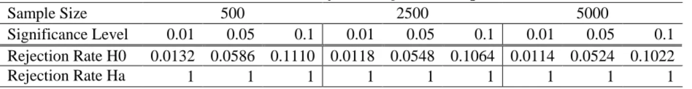
Table 1: VECM Causality Test Rejection Frequencies
Sample Size 500 2500 5000
Significance Level 0.01 0.05 0.1 0.01 0.05 0.1 0.01 0.05 0.1
Rejection Rate H0 b_12=0
0.0132 0.0586 0.1110 0.0118 0.0548 0.1064 0.0114 0.0524 0.1022 Rejection Rate Ha
b_12=0.2
1 1 1 1 1 1 1 1 1
The results in Table 1 show that our Wald test for Granger-causality in VECM has good size and power
under different significance levels and for various sample sizes. The rejection rate is 100% for all cases
17 that empirical size approaches the significance level as sample size increases, but it is already reasonably
close even with a sample size of only 500.
5.2.2 Bivariate GARCH Volatility Spillover Test Simulation Results
The data generating process is a bivariate GARCH (1, 1) as in Aguilar & Hill (2015):
𝑦𝑖,𝑡= ℎ𝑖,𝑡𝑧𝑖,𝑡,𝑧𝑖,𝑡~𝑁𝑜𝑟𝑚𝑎𝑙(0,1) (17)
[ℎ1,𝑡
2
ℎ2,𝑡2
] = [0.3
0.3] + [
0.3 𝑎12
0 0.3] [ 𝑦1,𝑡−12
𝑦2,𝑡−12
] + [0.6 𝑏12
0 0.6] [
ℎ1,𝑡−12
ℎ2,𝑡−12
] (18)
We simulate three levels of volatility spillover: no spillover, weak spillover, and strong spillover where
𝑎12 takes 0, 0.1, and 0.3 respectively and 𝑏12 takes 0, 0.3, and 0.6 respectively. We simulate 10,000
samples with sample size 1000, 2500, and 5000 for each volatility spillover level and each significance
level 1%, 5%, and 10%. Lags tested are 1, 2, 3, 4, 5, 10, 15, and 20. We set our initial values 𝑦1,02 =
𝑦2,02 = ℎ
1,02 = ℎ2,02 = 0. The results are reported in the tables below.
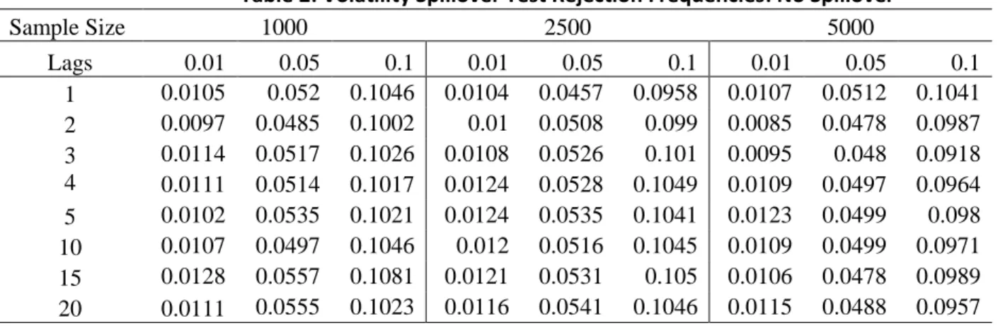
Table 2: Volatility Spillover Test Rejection Frequencies: No Spillover
Sample Size 1000 2500 5000
Lags 0.01 0.05 0.1 0.01 0.05 0.1 0.01 0.05 0.1
1 0.0105 0.052 0.1046 0.0104 0.0457 0.0958 0.0107 0.0512 0.1041 2 0.0097 0.0485 0.1002 0.01 0.0508 0.099 0.0085 0.0478 0.0987 3 0.0114 0.0517 0.1026 0.0108 0.0526 0.101 0.0095 0.048 0.0918 4 0.0111 0.0514 0.1017 0.0124 0.0528 0.1049 0.0109 0.0497 0.0964
5 0.0102 0.0535 0.1021 0.0124 0.0535 0.1041 0.0123 0.0499 0.098 10 0.0107 0.0497 0.1046 0.012 0.0516 0.1045 0.0109 0.0499 0.0971 15 0.0128 0.0557 0.1081 0.0121 0.0531 0.105 0.0106 0.0478 0.0989 20 0.0111 0.0555 0.1023 0.0116 0.0541 0.1046 0.0115 0.0488 0.0957
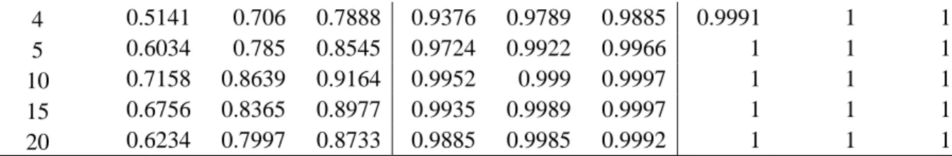
Table 3: Volatility Spillover Test Rejection Frequencies: Weak Spillover
Sample Size 1000 2500 5000
Lags 0.01 0.05 0.1 0.01 0.05 0.1 0.01 0.05 0.1
18
4 0.5141 0.706 0.7888 0.9376 0.9789 0.9885 0.9991 1 1
5 0.6034 0.785 0.8545 0.9724 0.9922 0.9966 1 1 1
10 0.7158 0.8639 0.9164 0.9952 0.999 0.9997 1 1 1
15 0.6756 0.8365 0.8977 0.9935 0.9989 0.9997 1 1 1
20 0.6234 0.7997 0.8733 0.9885 0.9985 0.9992 1 1 1
Table 4: Volatility Spillover Test Rejection Frequencies: Strong Spillover
Sample Size 1000 2500 5000
Lags 0.01 0.05 0.1 0.01 0.05 0.1 0.01 0.05 0.1
1 0.1713 0.3222 0.4139 0.4001 0.6072 0.7049 0.717 0.8691 0.9159 2 0.3931 0.5886 0.6897 0.815 0.9202 0.9554 0.9888 0.9978 0.9999
3 0.5934 0.7648 0.8422 0.9627 0.9887 0.9937 0.9999 1 1
4 0.7136 0.8577 0.9078 0.9904 0.998 0.9992 1 1 1
5 0.7858 0.9005 0.9388 0.9976 0.9996 0.9998 1 1 1
10 0.8629 0.946 0.971 0.9998 0.9999 1 1 1 1
15 0.831 0.9303 0.9612 0.9997 0.9998 1 1 1 1
20 0.7866 0.9038 0.9437 0.9992 0.9998 0.9998 1 1 1
From the no spillover case in Table 2, we see that the test has good size for all three sample sizes and all
significance levels. From the weak spillover case in Table 3, we see that the test has low power,
especially for lower lags, when the sample size is 1000. When we increase the sample size to 2500 and
5000, the test has reasonably high power starting from the 3rd lag. In the strong spillover case, power is
generally higher than the weak spillover case but is still low when sample size is 1000. It has high power
after the 2nd lag for sample size 2500 and 5000. This indicates that our spillover test works is expected to
perform well at any lag, including small lags. The sample sizes for both the pre-crash period and the
post-crash period are 3283. However, we will not be able to perform this spillover test in our rolling window
analysis as the window size will be too small for the test to have reasonable power.
6. Empirical Results
6.1 VECM Results
We estimate our VECM model with a standard Engle-Granger 2-step OLS method (Engel and Granger,
1987). Furthermore, it is a stylized fact that financial time series often display heteroscedasticity, and we
19 so we estimated a heteroscedastic-robust covariance matrix according to White (1980). We then perform
Wald test using the obtained covariance matrix.
[Table 5]
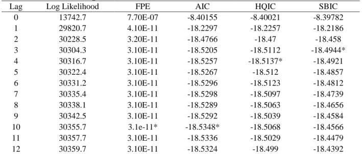
From Table 5, we observe that AIC reaches its minimum at the 10th VAR lag. The actual lag in VECM is
then 1 less than its VAR lag. So we choose total lag j to be 9.
[Table 6]
[Table 7]
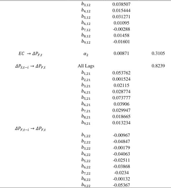
Table 6 and Table 7 report the results from the Wald tests for the pre-crash period and post-crash period.
For pre-crash period the adjustment term 𝛼1 is significant at 10% level, while 𝛼2 is not significant at any
meaningful level. For post-crash period, we obtain similar results. This provides evidence that price
adjustments only take place in the stock market. In other words, if the stock prices and the futures prices
deviate, the stock prices will move closer to futures prices while futures prices can be seen as exogenous.
Coefficients for lagged returns also corroborate the above conclusion. We test the hypothesis whether past
futures return Granger-causes present stock returns. In other words, we test whether 𝑏𝑖,12= 0 for all
lags 𝑖 with a Wald test. For both the pre-crash period and the post-crash period, the p-values are
practically zero. We also test whether past stock prices Granger-causes present futures prices. For the
pre-crash period, we see a P-value of 0.035, and it suggests that stock return also Granger-causes futures
returns. However, during the post-crash period there is no evidence for the above relationship at any
meaningful significance level as the P-value is 0.82. Comparing across markets, we can conclude that the
Granger-causality from the futures market to the stock market is much stronger than the other way
around. Comparing across time, we see that either the market crash itself or Chinese government
regulations diminished the impact of the stock market on the futures market; however, the futures market
still has a statistically significant impact on the stock market.
20 [Figure 2]
Figure 1 and Figure 2 report the P-values from the rolling window analysis. We pick window size m=500.
We observe that p-values for the Granger non-causality test from lagged futures returns to stock returns
are practically zero for all subsamples except for the periods during which Chinese government adopted
new regulatory policies on futures trading, hence there is strong evidence of causality at any standard
level of significance. It is especially worth noting that data around observation 4000 corresponds to the
days around July 6, and observation 6000 corresponds to late August. The P-values spikes at exactly the
same time period when new barriers to entry are introduced. In other words, futures prices have no
prediction power in the few days following the introduction of each new barriers. On the other hand,
P-values for the test from lagged stock returns to futures returns vary across time but is hardly lower than
the 0.05 threshold. This conforms to what is suggested by our theoretical model: changes in futures
returns causes change in stock returns while stock returns should have little predictive power on futures
returns.
6.2 Volatility Spillover Results
[Table 8]
Table 8 presents the result of volatility spillover Q-tests. It shows that volatility transmission from the
futures market to the stock market is significant if we only consider the first lag. Volatility transmission
from the stock market to the futures market is significant for the first two lags. P values are slightly
smaller for spillover from stock market to the futures market than the other way around. The results show
weak evidence for volatility spillover from the futures market to the stock market before the market crash
and a slightly stronger spillover from the stock market to the futures market. After the stock market crash,
there is only evidence for spillover from the futures market to the stock market, but no evidence for the
other direction.
21 [Figure 4]
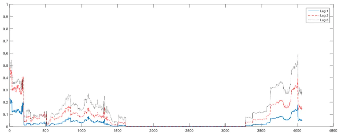
Figure 3 and Figure 4 present the results from the rolling window analysis with a window size of 2500.
We report the P-values for the first three lags as our simulation study indicates that they have the proper
size and power. We can observe from Figure 3 that there is significant volatility spillover form the futures
market to the stock market at the first lag during the larger part of the pre-crash period. P-value goes up
after the market crash. Comparing Figure 4 with Figure 3, we find that P-values are generally higher in
Figure 3 except for a brief period. This indicates that volatility spillover from the futures market to the
stock market is stronger than that in the other direction in most sub-periods.
We note that the full-sample results from our volatility spillover tests differ from price causality results.
Whereas futures prices show a much stronger effect on the stock prices, futures volatilities have a weaker
effect on stock volatilities. Moreover, mean causality from the stock market to the futures market is never
significant for any extended period of time as shown in the rolling window analysis. On the contrary,
there is significant volatility spillover from the stock market to the futures market during a period of 1000
samples, or approximately 20 trading days. This might imply that volatility transmission follow a
different mechanism than price transmission. This hypothesis, however, needs further support from
theoretical studies.
6.3 Volatility Spillover Bootstrap
Though our simulation results show that our volatility spillover tests work well if the data generation
process is bivariate GARCH; however, it is highly unlikely that our empirical data comes from such a
simplistic process. More specifically, our Q test requires the GARCH residuals to be not only
uncorrelated but also independent, and we cannot guarantee independence without prior knowledge about
the true data generating process. Therefore we adopt a more robust test for volatility spillover using the
dependent wild bootstrap method introduced in Shao (2010), where independence is not assumed.
22 1. We divide our centered squared standardized residuals obtained from step (2) of our previous
volatility spillover test, {𝑢̂𝑆,𝑡} and {𝑢̂𝐹,𝑡} , into blocks of size 𝑏 = ⌊√𝑛⌋ where 𝑛 is the sample size.
There will then be 𝑘 = ⌊𝑛
𝑏⌋ blocks in total for each set of residuals. Note that it is very likely that
𝑛 mod (𝑏) ≠ 0, so we need to append the remaining data into the last block and its size turns
into 𝑏∗= 𝑏 + 𝑛 mod (𝑏).
2. We generate i.i.d. Normal (0, 1) random numbers {𝑧𝑖| 𝑖 = 1,2, … , 𝑘 }. Then we define 𝑤𝑡=
𝑧𝑖 𝑓𝑜𝑟 𝑡 ∈ { 𝑡 | 𝑢̂𝑖,𝑡∈ 𝑖𝑡ℎ 𝑏𝑙𝑜𝑐𝑘} such that 𝑤1= 𝑧1, 𝑤2= 𝑧1, … , 𝑤𝑏+1 = 𝑧2, … , 𝑤2𝑏+1= 𝑧3, and
etc.
3. We calculate our bootstrapped correlation coefficient 𝜌̂𝑑𝑤𝑏(ℎ) for lag ℎ according to the formula
below where 𝑥𝑡=𝑢̂𝑆,𝑡 and 𝑦𝑡 =𝑢̂𝐹,𝑡:
𝜌̂𝑑𝑤𝑏(ℎ) = 1
√1
𝑛∑𝑛𝑡=1(𝑥𝑡𝑦𝑡− 𝑥̅ 𝑦𝑡 ̅ )𝑡 2
∙1
𝑛∑ 𝑤𝑡(𝑥𝑡𝑦𝑡−ℎ−
1
𝑛∑ 𝑥𝑡𝑦𝑡−ℎ
𝑛
𝑡=1+ℎ )
𝑛
𝑡=1+ℎ (19)
4. We repeat the above steps 𝑀 times to obtain 𝑀 sample correlations 𝜌̂𝑑𝑤𝑏(ℎ) for each lag h, and
calculate the Ljung-Box Q statistics 𝑄𝑖𝑑𝑤𝑏(ℎ) 𝑓𝑜𝑟 𝑖 = 1, … , 𝑀 using the same formula as in step
(3) of our original test method. Finally we calculate the P-value 𝑃̂𝑀𝑑𝑤𝑏(ℎ) where ℎ denotes the
maximum lag. 𝐼(∙) is an indicator function, and 𝑄(ℎ) is exactly the same value in step (3).
𝑃̂𝑀𝑑𝑤𝑏(ℎ) =
1
𝑀∑ 𝐼 (𝑄𝑖
𝑑𝑤𝑏(ℎ) ≥ 𝑄(ℎ))
𝑀
𝑖=1 (20)
6.3.1 Bootstrap Simulation
We investigate the size and power of our bootstrap method through simulation. There are 10,000 samples,
and M=1000 bootstrap samples. We report the rejection rate for those 10,000 repetitions. The data
generating process is the same as the one in our previous volatility spillover simulation. The results are
23 Table 9: Volatility Spillover Bootstrap Rejection Frequencies: No Spillover
Sample Size 1000 2500 5000
Lags 0.01 0.05 0.1 0.01 0.05 0.1 0.01 0.05 0.1
1 0.0149 0.0614 0.1166 0.0105 0.0497 0.1074 0.0106 0.0529 0.1002 2 0.0098 0.0515 0.1112 0.0079 0.0469 0.1017 0.0094 0.0503 0.0993 3 0.0079 0.0506 0.1047 0.0083 0.0479 0.0998 0.0096 0.0495 0.0991 4 0.0075 0.0458 0.1044 0.0075 0.047 0.0999 0.0093 0.0485 0.0964
5 0.0061 0.0451 0.1003 0.0075 0.0467 0.1053 0.0081 0.0468 0.097 10 0.0061 0.0446 0.0949 0.0077 0.0451 0.0962 0.0069 0.0459 0.0952 15 0.0051 0.0388 0.0927 0.0069 0.0435 0.0928 0.0074 0.0471 0.0883 20 0.0044 0.0372 0.0854 0.0076 0.0431 0.0902 0.0072 0.0473 0.0894
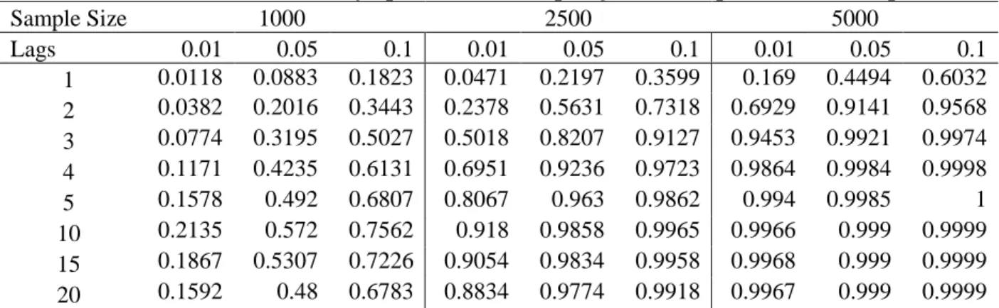
Table 10: Volatility Spillover Bootstrap Rejection Frequencies: Weak Spillover
Sample Size 1000 2500 5000
Lags 0.01 0.05 0.1 0.01 0.05 0.1 0.01 0.05 0.1
1 0.0118 0.0883 0.1823 0.0471 0.2197 0.3599 0.169 0.4494 0.6032 2 0.0382 0.2016 0.3443 0.2378 0.5631 0.7318 0.6929 0.9141 0.9568 3 0.0774 0.3195 0.5027 0.5018 0.8207 0.9127 0.9453 0.9921 0.9974 4 0.1171 0.4235 0.6131 0.6951 0.9236 0.9723 0.9864 0.9984 0.9998
5 0.1578 0.492 0.6807 0.8067 0.963 0.9862 0.994 0.9985 1
10 0.2135 0.572 0.7562 0.918 0.9858 0.9965 0.9966 0.999 0.9999 15 0.1867 0.5307 0.7226 0.9054 0.9834 0.9958 0.9968 0.999 0.9999 20 0.1592 0.48 0.6783 0.8834 0.9774 0.9918 0.9967 0.999 0.9999
Table 11: Volatility Spillover Bootstrap Rejection Frequencies: Strong Spillover
1000 2500 5000
Lags 0.01 0.05 0.1 0.01 0.05 0.1 0.01 0.05 0.1
1 0.027 0.1618 0.3061 0.1526 0.4472 0.6168 0.4846 0.7974 0.8934 2 0.0824 0.3474 0.5254 0.505 0.8231 0.9157 0.9295 0.9906 0.9973 3 0.1646 0.4998 0.6883 0.767 0.9516 0.984 0.9882 0.9985 0.9997 4 0.2344 0.6088 0.7832 0.8875 0.9841 0.9956 0.9942 0.999 0.9998 5 0.2879 0.6699 0.8309 0.9285 0.9914 0.9978 0.9961 0.9993 0.9999
10 0.3581 0.7366 0.8778 0.9681 0.9959 0.9982 0.9976 0.9995 1
15 0.3178 0.6974 0.8466 0.9642 0.9952 0.9982 0.9975 0.9995 1
20 0.2752 0.6476 0.8123 0.9588 0.9945 0.9978 0.9974 0.9996 1
The “No-Spillover” case show that our test statistics has a size close to its theoretical rejection rate for the
first two lags but significantly smaller size at higher lags. The rejection rates, however, monotonically
improve with an increased sample size. In the “Weak-Spillover” and “Strong-Spillover” cases, we find
24 sample size is 2500 and 5000. This suggests that our test statistics have proper size and power when the
sample size is larger than 2500 and when we look at the second or the third lags.
6.3.2 Bootstrap Results
[Table 12]
By looking at the second and the third lags suggested by our simulation, we find that our bootstrap results
corroborate with the results found in Table 4. There is some evidence for bidirectional volatility spillovers
before the stock market crash, and the spillover from the stock market to the futures market is stronger
than the other direction. After the crash, there is still evidence for volatility spillover from the futures
market to the stock market but no evidence for the other direction. This reinforces our belief that volatility
spillover follows a different mechanism than causality in prices.
7. Conclusion
Using high frequency data, we examine the causal relationship in prices and in volatility between China’s
CSI 300 stock index and its futures contract. Our data cover both a period of low barriers to entry and a
period of rising barriers. In this way, we not only examines if the temporal relationship between the two
assets has become more aligned with those observed in developed markets six years after the initial study
by Yang, Yang, and Zhou (2010), but also provides empirical evidence for the financial theory that high
barriers of entry hurts price discovery performance of the futures market. Specifically, we test for Granger
causality between the prices in the two markets using a vector error correction model (VECM) and test
for volatility spillovers with a Q-test based on Ljung and Box (1978) and a test proposed by Hong (2001).
We further validate our spillover test results by performing a more robust dependent wild bootstrap
method introduced in Shao (2010).
We find that changes in CSI 300 futures prices consistently Granger-cause changes in CSI stock prices
during the pre-crash period. Significant bidirectional volatility spillover exists during the pre-crash period.
25 market and the stock market has become aligned with those observed in developed markets. After the
stock market crash, the futures price has a less consistent effect on the stock price. Futures prices can help
predict stock prices in some sub-periods but not in others. In the first few days following the introduction
of each new barriers, futures prices invariably have no prediction power. There is still significant
volatility spillover from the futures market to the stock market after the crash, but there is no evidence for
the other direction. The above results might provide evidence that barriers to entry indeed affects the price
discovery performance of the futures market, confirming what is suggested by financial theories.
Furthermore, the results might indicate that changes in prices and changes in volatility are transmitted
through different channels between the stock market and the futures market. The plausibility of latter
26 References
Aguilar, M., & Hill, J. B. (2015). Robust score and portmanteau tests of volatility spillover. Journal of Econometrics, 184(1), 37-61.
Booth, G., So, R., & Tse, Y. (1999). Price discovery in the German equity index derivatives markets.
Journal of Futures Markets,19(6), 619-643.
Box, G. E., & Pierce, D. A. (1970). Distribution of residual autocorrelations in autoregressive-integrated moving average time series models. Journal of the American statistical Association, 65(332), 1509-1526.
Dufour, J. M., & Renault, E. (1998). Short run and long run causality in time series: theory. Econometrica, 66(5), 1099-1125.
Engle, R. F. and Granger, C. W. J. (1987). Co-Integration and Error-Correction: Representation, Estimation, and Testing. Econometrica, 55, pp. 251–276.
Engle, R., & Kroner, K. (1995). Multivariate Simultaneous Generalized ARCH. Econometric Theory, 11(1), 122-122.
Fama, E. F. (1970). Efficient capital markets: A review of theory and empirical work. The Journal of Finance, 25(2), 383-417.
Fleming, J., Ostdiek, B., & Whaley, R. E. (1996). Trading costs and the relative rates of price discovery in stock, futures, and option markets. Journal of Futures Markets, 16(4), 353-387.
Granger, C. W. (1969). Investigating causal relations by econometric models and cross-spectral methods. Econometrica, 424-438.
Granger, C. W., & Newbold, P. (1974). Spurious regressions in econometrics. Journal of Econometrics, 2(2), 111-120.
Hong, Y. (1996). Testing for independence between two covariance stationary time series. Biometrika,
83, 615–625.
Hong, Y. (2001). A test for volatility spillover with application to exchange rates. Journal of Econometrics, 103(1), 183-224.
Johansen, S. (1991). Estimation and Hypothesis Testing of Cointegration Vectors in Gaussian Vector Autoregressive Models. Econometrica,59(6), 1551-1551.
Koutmos, G., & Tucker, M. (1996). Temporal relationships and dynamic interactions between spot and futures stock markets. Journal of Futures Markets,16(1), 55-69.
Ljung, G. M., & Box, G. E. (1978). On a measure of lack of fit in time series models. Biometrika, 65(2), 297-303.
27 So, R., & Tse, Y. (2004). Price discovery in the hang seng index markets: Index, futures, and the tracker fund. Journal of Futures Markets,24(9), 887-907.
Stoll, H., & Whaley, R. (1990). The Dynamics of Stock Index and Stock Index Futures Returns. The Journal of Financial and Quantitative Analysis,25(4), 441-441.
Tse, Y. (1999). Price discovery and volatility spillovers in the DJIA index and futures markets. Journal of Futures Markets,19(8), 911-930.
White, Halbert (1980). A Heteroskedasticity-Consistent Covariance Matrix Estimator and a Direct Test for Heteroskedasticity. Econometrica, 48(4), 817–838.
28 Table 5. VECM Lag (The reported lag is the underlying lag in its VAR form and will be 1 lag more than the actual VECM lag)
Lag Log Likelihood FPE AIC HQIC SBIC
0 13742.7 7.70E-07 -8.40155 -8.40021 -8.39782
1 29820.7 4.10E-11 -18.2297 -18.2257 -18.2186
2 30228.5 3.20E-11 -18.4766 -18.47 -18.458
3 30304.3 3.10E-11 -18.5205 -18.5112 -18.4944*
4 30316.7 3.10E-11 -18.5257 -18.5137* -18.4921
5 30322.4 3.10E-11 -18.5267 -18.512 -18.4857
6 30331.2 3.10E-11 -18.5296 -18.5123 -18.4812
7 30335.4 3.10E-11 -18.5298 -18.5097 -18.4739
8 30338.1 3.10E-11 -18.5289 -18.5063 -18.4656
9 30342.5 3.10E-11 -18.5292 -18.5039 -18.4584
10 30355.7 3.1e-11* -18.5348* -18.5068 -18.4566
11 30357.7 3.10E-11 -18.5336 -18.5029 -18.4479
12 30359.7 3.10E-11 -18.5324 -18.499 -18.4392
Note: This table reports the log likelihood and relevant information criterion for VECM with different underlying VAR lags. We pick the number of lags by minimizing AIC, so lag 10 is selected. * indicate the minimum for each information criterion.
Table 6. VECM Estimated Parameters-Pre-Crash
Coefficient Value P-value
𝐸𝐶 → 𝛥𝑃𝑆,𝑡 𝛼1 -0.01188 0.0825
𝛥𝑃𝑆,𝑡−𝑖→ 𝛥𝑃𝑆,𝑡
𝑏1,11 -0.48418
𝑏2,11 -0.2236
𝑏3,11 -0.09625
𝑏4,11 -0.0736
𝑏5,11 -0.00891
𝑏6,11 -0.01854
𝑏7,11 -0.06959
𝑏8,11 -0.08093
𝑏9,11 -0.11133
𝛥𝑃𝐹,𝑡−𝑖→ 𝛥𝑃𝑆,𝑡 All Lags 0
𝑏1,12 0.496977
𝑏2,12 0.207368
𝑏3,12 0.102724
𝑏4,12 0.069703
𝑏5,12 0.063191
𝑏6,12 0.038888
𝑏7,12 0.072941
𝑏8,12 0.079499
29
𝐸𝐶 → 𝛥𝑃𝐹,𝑡 𝛼2 0.00423 0.6163
𝛥𝑃𝑆,𝑡−𝑖 → 𝛥𝑃𝐹,𝑡 All Lags 0.0352
𝑏1,21 0.008261
𝑏2,21 0.056169
𝑏3,21 0.035088
𝑏4,21 0.042147
𝑏5,21 0.054152
𝑏6,21 0.040237
𝑏7,21 -0.021
𝑏8,21 -0.0165
𝑏9,21 -0.08384
𝛥𝑃𝐹,𝑡−𝑖→ 𝛥𝑃𝐹,𝑡
𝑏1,22 -0.05525
𝑏2,22 -0.06942
𝑏3,22 -0.03435
𝑏4,22 -0.01666
𝑏5,22 -0.02722
𝑏6,22 -0.03709
𝑏7,22 0.007815
𝑏8,22 0.005418
𝑏9,22 0.04194
Note: This table reports the estimated value of VECM parameters with 9 lags (or 10 underlying VAR lags). Chi-square statistics and its associated p-value are the results of Wald tests. Since we test for the null-hypothesis that the diagonal terms for all lags are zero, we only provide test statistics in the all lags section. Each lag is not individually tested. The first column indicates the direction of Granger (non)-causality implied by the parameters.
Table 7. VECM Estimated Parameters-Post-Crash
Coefficient Value P-value
𝐸𝐶 → 𝛥𝑃𝑆,𝑡 𝛼1 -0.01456 0.0238
𝛥𝑃𝑆,𝑡−𝑖→ 𝛥𝑃𝑆,𝑡
𝑏1,11 -0.27234
𝑏2,11 -0.08783
𝑏3,11 0.00442
𝑏4,11 -0.0186
𝑏5,11 0.00214
𝑏6,11 0.000802
𝑏7,11 0.026884
𝑏8,11 -0.01323
𝑏9,11 0.004476
𝛥𝑃𝐹,𝑡−𝑖→ 𝛥𝑃𝑆,𝑡 All Lags 0
𝑏1,12 0.280807
30
𝑏3,12 0.038507
𝑏4,12 0.015444
𝑏5,12 0.031271
𝑏6,12 0.01095
𝑏7,12 -0.00288
𝑏8,12 0.01458
𝑏9,12 -0.01601
𝐸𝐶 → 𝛥𝑃𝐹,𝑡 𝛼2 0.00871 0.3105
𝛥𝑃𝑆,𝑡−𝑖 → 𝛥𝑃𝐹,𝑡 All Lags 0.8239
𝑏1,21 0.053762
𝑏2,21 0.001524
𝑏3,21 0.02115
𝑏4,21 0.028774
𝑏5,21 0.073777
𝑏6,21 0.03906
𝑏7,21 0.029947
𝑏8,21 0.018665
𝑏9,21 0.013234
𝛥𝑃𝐹,𝑡−𝑖→ 𝛥𝑃𝐹,𝑡
𝑏1,22 -0.00967
𝑏2,22 -0.04847
𝑏3,22 -0.00179
𝑏4,22 -0.04063
𝑏5,22 -0.02511
𝑏6,22 -0.03868
𝑏7,22 -0.0234
𝑏8,22 -0.00132
𝑏9,22 -0.05367
Note: This table reports the estimated value of VECM parameters with 9 lags (or 10 underlying VAR lags). Chi-square statistics and its associated p-value are the results of Wald tests. Since we test for the null-hypothesis that the diagonal terms for all lags are zero, we only provide test statistics in the all lags section. Each lag is not individually tested. The first column indicates the direction of Granger (non)-causality implied by the parameters.
Table 8. Volatility Spillover Test Results
Time Period Pre-Crash Post-Crash
Lags ( j) Futures to Stock Stock to Futures Futures to Stock Stock to Futures
P-value P-value P-value P-value
1 0.0180 0.0177 0.0105 0.6308
2 0.0563 0.0474 0.0362 0.8753
3 0.0838 0.0898 0.0832 0.9662
4 0.0766 0.1444 0.1254 0.8436
31
6 0.1804 0.2759 0.2914 0.9364
7 0.2582 0.2813 0.3740 0.9678
8 0.3413 0.2657 0.4422 0.9811
9 0.4357 0.2682 0.5299 0.9913
10 0.5237 0.2713 0.6219 0.9894
11 0.4775 0.2445 0.7046 0.9946
12 0.5598 0.2447 0.7771 0.9968
13 0.5502 0.2707 0.8249 0.9973
14 0.5034 0.2961 0.8720 0.9987
15 0.5786 0.2354 0.9103 0.9990
16 0.6433 0.2729 0.9063 0.9984
17 0.4835 0.2895 0.9078 0.9984
18 0.5501 0.3296 0.9280 0.9992
19 0.4825 0.1838 0.9439 0.9995
20 0.5262 0.0647 0.9514 0.9997
Note: This table reports the P-values for the volatility spillover tests on both the pre-crash period and the post-crash period. H0 is that there is no volatility spillover. Rejection of H0 at lag j indicates the existence of volatility spillover up till the jth lag.
Table 12. Bootstrap Volatility Spillover Test Results
Time Period Pre-Crash Post-Crash
Lags ( j) Futures to Stock Stock to Futures Futures to Stock Stock to Futures
P-value P-value P-value P-value
1 0.0254 0.0187 0.0076 0.6481
2 0.0649 0.0472 0.0319 0.8897
3 0.0774 0.0678 0.0905 0.9712
4 0.0612 0.0996 0.13 0.8756
5 0.134 0.1872 0.25 0.94
10 0.5567 0.3025 0.6827 0.993
15 0.585 0.2281 0.928 0.9991
20 0.5647 0.0608 0.9645 0.9999
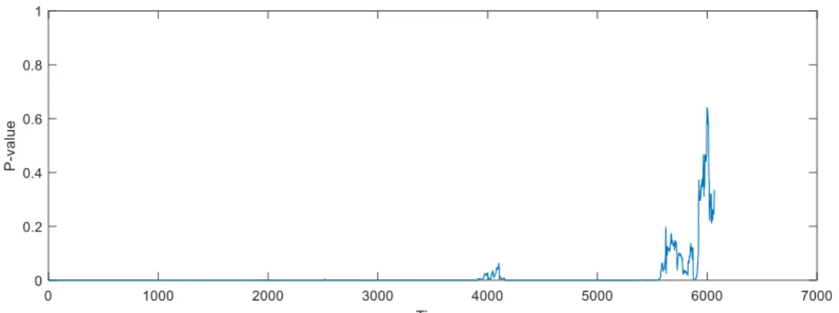
32 Figure 1. Rolling Window P-value for Granger non-causality from Index Futures Returns to Index Returns
Note: We perform rolling window analysis to test Granger non-causality with a window size of 500. Each point on the line is the p-value of the Wald test for the sub-period of 500 5-minute periods. Time is measured in 5-min intervals. So 1000 is the 1000th 5-minute interval in the data. It is worth noting that data around 4000 corresponds to the days around July 6, and 6000 corresponds to late August. The P-values spikes at exactly the same time period when new barriers to entry are introduced.
Figure 2. Rolling Window P-value for Granger non-causality from Index Returns to Index Futures Returns
33 Figure 3. Rolling Window P-value for Volatility Spillover from Index Futures Returns to Index Returns
Note: We perform rolling window analysis to test volatility spillover from the futures market to the stock market with a window size of 2500. Each point on the line is the p-value of the Q test for the sub-period of 2500 5-minute periods. The largs being reported are the first three lags.
Figure 4. Rolling Window P-value for Volatility Spillover from Index Futures Returns to Index Returns
34 Appendix
Timetable of CFFE Policies after June 2015 Market Crash (only those directly affecting the CSI 300 are included)
Announcement Date
Effective
Date Policy
7/3 7/6 Limit single account intraday buy/sell volume to 1200 contracts
7/31 8/3 Start charging a fee of 1 Yuan for placing a buy/sell order or cancelling an existing order
8/25 8/26 Increase transaction fee to 1.5/10,000 of total transaction amount
8/25 8/26-28 Increase margin requirement from 10% to 12%, 15%, and 20% in the next three days
8/28 8/31 Increase margin requirement to 30%
9/2 9/7 Increase transaction fee to 23/10,000 of total transaction amount