Thesis

Acknowledgements

I am grateful to Dr. Klara Peter for helpful comments and suggestions, as well as for instilling in me a proactive approach towards the completion of this project. I am especially grateful to Dr. Lutz Hendricks for his immeasurable contributions at every stage of this honors thesis. If this paper does not embarrass UNC’s undergraduate economics department, it will be due to Dr. Hendricks’ willingness to share his expertise and his patience while doing so.

2 Abstract

3 I. Introduction

Traditional neoclassical growth models feature a production function that maps a country’s labor and capital inputs to its economic output. However, models focused only on these input factors cannot explain cross-country income variation, as capital and labor stocks between rich and poor countries are not wide enough to justify the differences in their per capita output. Standard growth models are forced to account for the unexplained residual with a

catchall variable commonly referred to as Total Factor Productivity (TFP). The existence of this residual has motivated the creation of a variety of theories meant to more accurately model input factors and chip away at this “measure of our ignorance.”

Human capital models have traditionally attempted to reduce reliance on TFP by

weighting labor stocks according to education levels, effectively widening the difference in labor inputs between rich and poor countries. While this is an intuitive approach, the effectiveness of human capital models are limited for reasons including the difficulty of measuring human capital, the relatively small amount of cross-country output variation that measurable human capital differences can account for, and the difficulty in proving causality between education levels and output.

4 While most human capital approaches focused on the substitution elasticity between labor inputs assume that labor is divided into one skilled group and one unskilled group, Jones (2014) produces a generalized human capital aggregator with n skill types to create a more adaptable model. His general approach extends the literature by producing an aggregator that takes advantage of the developments discussed above, while also nesting standard human capital models as a special case. This allows him to compare the two approaches directly, and establish that current human capital models provide only a lower bound on cross-country human capital variation.

Although this approach is mathematically sound and can decrease reliance on TFP, no work has been done to establish the limits of this approach with regards to the manipulation of the substitution elasticity between labor inputs. If such a limit is found to exist, then human capital models may not be able to reduce reliance on TFP and another route will have to be pursued to explaining cross-country income differences; otherwise, cross-country income

differences may be fully explained within a human capital framework. With this in mind, we see that there is value in determining whether an upper bound on human capital variation exists inside a generalized framework.

Our paper finds that, although generalized human capital models can accurately model cross-country income differences when the substitution elasticity between labor inputs falls within a desired range, such accuracy comes at the cost of predicting the existence of skill premiums in undeveloped countries that far outstrip such premiums in developed countries. This forces generalized human capital models to conclude that human capital flight should be

5 Uruguay in order to “cash in” on those countries’ skill premiums. This introduces a possible upper bound on the accuracy of generalized human capital models; these models may only be able to manipulate the substitution elasticity between skill groups until the relative price of skilled labor between rich and poor countries reaches parity. If this result is correct, it implies that a theory of TFP is necessary to accurately model cross-country income differences.

The order of this paper, then, is as follows. We first review the literature and discuss the rationale behind generalized human capital accounting. We then produce a generalized human capital aggregator under CES specifications and conduct an accounting exercise, imposing weak restrictions on skill prices implied by the model to derive an upper bound on the contribution of human capital to income gaps. These restrictions will follow from the a priori assumption that no skill class of workers should have a higher wage in a poor country than in a rich one.

II. Literature Review

While human capital models have expanded in several directions, they are all in pursuit of the same goal: find a way to increase variation in cross-country capital and human capital stocks, such that rich countries get more of these inputs or poor countries get less. For instance, Francesco Caselli (2005) provides an overview of attempts to augment human capital’s role in explaining cross-country income variation based on the efficiency with which factor inputs are used. Metrics such as the quality of physical capital, the health of a nation’s workforce, and the quality of schooling are considered as possible candidates to decrease reliance on TFP.

6 unskilled workers are perfect substitutes, and find that there is a skill bias in the way rich and poor countries implement technologies. This leads to their assertion that rich countries use highly educated workers more effectively than poor countries, but use less educated workers relatively and, possibly, absolutely less effectively.

This is an important result, as it provides evidence that the relative amount of skilled or unskilled labor can affect wage rates, at least insofar as it obliges countries to implement

technologies that augment either skilled or unskilled labor. It also asserts that assumptions made by standard human capital models may lead to biased results, and that adjusting labor inputs for quality increases can reduce the contribution of TFP.

Bowlus and Robinson (2012) present a different approach to extending Human Capital models by producing a more accurate measure of the components of human capital: its price and quantity. They identify these components separately by breaking down the labor input into three types, dependent on their education levels. This alone is a break from previous literature, which has tended to compare only low-skilled and high-skilled workers, and had usually defined “low skilled” workers as only those possessing no education.

7 This research is insightful, because it provides firmer proof that a country’s output may be dependent not only on its capital stock and the quality of its workers, but again on the relative amount of skilled and unskilled workers in an economy. The paper also provides a way to more accurately measure human capital, and takes a step in the direction of generalizing the number of labor classes in an economy. The findings also note that as the number of labor classes increases from two to three, the effect of relaxing the assumption of perfect substitution between labor classes to augment cross-country human capital variation becomes greater.

These approaches have been expanded by Jones (2014), who has produced a generalized human capital model that is able make use of recent advances in the literature while nesting standard human capital models as a special case – allowing a direct comparison between the two approaches. Jones’ generalized human capital aggregator splits the labor input into n subgroups, divided with reference to observed education levels. He then builds off the work of Caselli by making two claims: That workers with different levels of human capital are imperfect substitutes, and that the marginal product of uneducated workers can be augmented by complementary effects between high and low skilled workers.

Jones’ second claim provides his model with much of its bite. By pointing out that uneducated workers can see their productivity increase as the number of educated workers increases, Jones introduces a possible new bias in previous human capital models. This

8 Jones’ model provides the most direct evidence that standard human capital models are biased, and that they provide only a lower bound on human capital variation. He finds that when skilled and unskilled labor have a substitution elasticity of 1.5, reliance on TFP is eliminated. If it is found that Jones’ model is theoretically sound, then human capital may provide the way to explaining TFP. However, if an upper bound on human capital variation can be established, then another explanation must be found to explain cross-country income differences.

With the recent mathematical success of generalized human capital aggregators, one might think that these models are ever closer to eliminating reliance on TFP. But the notion that the cross-country income gaps we see today are caused by inelastic labor groups presents a variety of problems. For instance, if human capital is the primary driver behind productivity, then skilled workers who immigrate to rich countries from poor ones should hardly see an earnings gain. The fact that this implication contradicts what we see in the world today implies that there are other important factors that must be responsible for income differences, such as social and legal institutions that are better accounted for by TFP than Human Capital.

9 Finally, the assumption that high and low skilled workers are not substitutable, combined with the assumption that highly skilled workers can increase the marginal productivity of human capital services, implies that there must be very large skill premiums in poor countries. This raises two problems for human capital models: What is preventing human capital accumulation in poor countries, and why are educated workers not migrating to poor countries to “cash in” on these large skill premiums?

III. Theoretical Model

A Review of Jones’ Generalized Approach

Having provided an overview of the existing literature surrounding generalized human capital models, there is still value in reviewing the work of Jones with more mathematical rigor. As our CES aggregator must be of the same spirit as Jones’ generalized aggregator, we commit ourselves now to reviewing his approach in some depth.

Jones begins by creating a human capital aggregator, where the human capital stock is equal to the sum total of the capital of the N different classes of workers. This provides the equation

𝐻 = 𝐺(𝐻₁, 𝐻₂, . . . , 𝐻_𝑛)

Where 𝐺(𝐻1, 𝐻2, . . . , 𝐻𝑛) is some aggregator such as CES. Jones shows that the above

equation is equivalent to

(1) 𝐻 = 𝐺₁(𝐻₁, 𝐻₂, . . . , 𝐻_𝑛)Ĥ

10 different amounts of Ĥ. We see that increasing/decreasing the term 𝐺1 has the effect of

increasing/decreasing the marginal value of a unit of unskilled labor Ĥ.

By rewriting (1), Jones provides a simple equation that allows us to see what inputs we need to measure the human capital stock:

𝐻 = 𝐺1*ℎ1∑

𝑤𝑖

𝑤1𝐿𝑖

𝑁 𝑖=1

where ℎ₁ denotes the human capital of unskilled workers and 𝐿_𝑖 denotes the quantity of workers

with the 𝑖 th level of human capital. This result points to the fact that, once we have used relative wages in an economy to convert workers into equivalent units of unskilled labor, we have to consider how the productivity of an unskilled worker depends on the skills of other workers, an effect encapsulated by 𝐺₁(Jones, 2014).

According to Jones, this shows why traditional human capital models have such trouble shaving down the total factor productivity scalar: variation in unskilled labor units is modest, so without accounting for the effect of the skills of other workers on the marginal output of

unskilled workers, relatively little of the large income variation we see between countries can be explained with human capital.

Jones continues by introducing a variable that can give a measurement of the bias

associated with current human capital models, defining Λ = 𝐻𝑅

𝐻𝑃

⁄

Ĥ𝑅

Ĥ𝑃

⁄ “as the ratio of true human

capital differences to the traditional calculation of human capital differences.” Using (*), this allows him to write the equivalent relationship

Λ =𝐺1𝑅 𝐺₁𝑃 ⁄

11 Jones introduces one final lemma with the introduction of a human capital aggregator

𝐻 = 𝐺(𝐻₁, 𝑍(𝐻₂, … , 𝐻_𝑁)),

where Z is a function representing the division of skilled labor. This provides Jones with evidence that traditional human capital accounting methods provide biased results, as he establishes that

(2) Λ =𝐺1𝑅 𝐺₁𝑃 ⁄ ≥ 1

If and only if

(3) 𝑍𝑅

𝐻₁𝑅

⁄ ≥ 𝑍𝑃

𝐻₁𝑃 ⁄

According to Jones, because (2) can be satisfied under a number of broad conditions, we see that previous growth models are likely biased and have yet to account for the actual human capital variation that exists across countries.

With this assertion providing a possible answer to the question of cross-country income variation, the type of model we must create to test Jones’ work is clear. Our model must be capable of separating the labor input into an arbitrary number of subclasses (i.e., skill classes), and our model must also be able to separate these skill classes into an arbitrary number of classes again (we refer to these “sub-subclasses” as human capital classes). Finally, our model must be capable of directly comparing cross-country income differences across a range of substitution elasticity values.

Producing a Human Capital Aggregator

With a prescribed direction that our model must follow, we now begin to develop our production function and human capital aggregator. Our first assumption is that there exists an aggregate production function of the form

12 where 𝐻 is aggregate human capital, 𝐾 is aggregate physical capital, and A is a scalar. We

assume that aggregators have constant returns to scale with regards to their capital inputs and provide a Cobb-Douglas production function for each country 𝐶:

𝑦_𝐶 = 𝑘_𝐶𝛼(𝐴_𝐶ℎ_𝐶)1−𝛼

We note that 𝛼, representing capital’s share of labor, is set equal to one third. Variables expressed as lowercase letters denote the fact that they are measured per worker.

Borrowing from the literature, we will assume that there exist human capital classes 𝐻_1,𝐶, 𝐻_2,𝐶, . . . , 𝐻_𝑁,𝐶, with workers in these classes possessing distinct levels of schooling.

We will use a constant elasticity of substitution (CES) specification to carry out our aggregation procedures; the CES production function we will use is of the form:

𝐶𝐸𝑆(𝑥_𝑖, µ, 𝜃) = [∑ (µ_{𝑖 𝑖}𝑥_𝑖)𝜃]1⁄𝜃

where µ_𝑖 is a weight on factor 𝑥_𝑖 and 𝜃 is the elasticity of substitution parameter. When this CES production function aggregates distinct groups X and Y, with inputs 𝑥_𝑖 and 𝑦_𝑖 respectively, we have the equation

𝐶𝐸𝑆(𝑋, 𝑌; µ, 𝜃) = [(µ₁𝑋)𝜃+ (µ₂𝑌)𝜃]1⁄𝜃

Because the purpose of this paper is to investigate the implications of relaxing the assumption of perfect substitutability between worker classes on cross-country human capital variation, we will define H as the aggregate human capital possessed by the class of unskilled workers Z1 and the class of skilled workers Z2. This provides the equation

13 with 𝜌 denoting the skill weight and 𝜀 the elasticity of substitution between the two classes of workers. We note that the skilled and unskilled human capital stocks themselves are aggregations of the human capital of worker classes 𝐻_1,𝐶, 𝐻_2,𝐶, . . . , 𝐻_𝑁,𝐶, with

𝑍_1,𝐶 = 𝐶𝐸𝑆(𝐻_1,𝐶, … , 𝐻_𝑆,𝐶; µ, 𝜃)

and

𝑍_2,𝐶 = 𝐶𝐸𝑆(𝐻_𝑆+1,𝐶, … , 𝐻_𝑁,𝐶; 𝜙, 𝜃),

with µ denoting the skill weight for unskilled workers in the worker classes 1-S, and 𝜙 denoting the skill weight for skilled workers in the worker classes S+1 - N. We divide workers into these groups with reference to observed education levels, so that a worker in class 𝑖 has less schooling than a worker in class 𝑖 + 1. With the aggregators in place, we note that the elasticity parameters for 𝑍₁ and 𝑍₂are the same, such that the substitution elasticity between skilled workers is the same as the elasticity between unskilled workers. The elasticity of substitution between skilled

and unskilled workers, however, is able to differ from the substitution elasticity within the two classes.

Assumptions Regarding the Labor Input

With a human capital aggregator specified, we move on to assumptions regarding the labor input. As is standard in neoclassical models, we assume factors are paid their marginal products, with the marginal product of capital input 𝑋_𝑗 described by the equation

𝜕𝑌𝐶

𝜕𝑋_𝑖,𝐶 = 𝑤𝑖,𝐶

14

1 ≤ 𝑖 ≤ 𝑆, is

𝑤_𝑖,𝐶 = 𝛿𝑌𝐶 𝛿𝐻_𝐶

𝛿𝐻_𝐶 𝛿𝑍_1,𝐶

𝛿𝑍_1,𝐶 𝛿𝐻_𝑖,𝐶

A parallel equation describes the unobserved price of type j labor, with type j labor belonging to the class of skilled workers. For 𝑆 + 1 ≤ 𝑗 ≤ 𝑁, we have

𝑤_𝑗,𝐶 = 𝛿𝑌𝐶 𝛿𝐻_𝐶

𝛿𝐻_𝐶 𝛿𝑍_2,𝐶

𝛿𝑍_2,𝐶 𝛿𝐻_𝑗,𝐶

For each worker class 𝐻_1,𝐶, 𝐻_2,𝐶, . . . , 𝐻_𝑁,𝐶, workers in the class 𝐻_𝑖,𝐶 possess an average level of human capital ℎ_𝑖,𝐶. Because of our assumption that factors are paid their marginal

products, we can define the wage bill of worker class 𝐻𝑖,𝐶, i.e., the sum of yearly earnings of all

workers in class 𝐻_𝑖,𝐶, with the equation

𝑤𝑎𝑔𝑒𝑏𝑖𝑙𝑙_𝑖,𝐶 = 𝑤_𝑖,𝐶ℎ_𝑖,𝐶𝐿_𝑖,𝐶 = 𝑤_𝑖,𝐶𝐻_𝑖,𝐶

This equation states that the wage bill of class 𝐻𝑖,𝐶 is the unseen price of that labor

type 𝑤_𝑖,𝐶, weighted by the average skill premium 𝐻_𝑖,𝐶 and total labor hours 𝐿_𝑖,𝐶. As many

economists note, while it is easy to measure the quantity of each labor type 𝐿_1,𝐶, 𝐿_2,𝐶, . . . , 𝐿_𝑁,𝐶,

neither the quality of each labor type ℎ1,𝐶, ℎ2,𝐶, . . . , ℎ𝑛,𝐶 nor the unseen price of labor can be

easily observed. With 𝑤_𝑖,𝐶 and ℎ_𝑖,𝐶 unknown, we will have to make additional assumptions to

proceed. But once we do, we will be able to measure ℎ𝑖,𝐶 for different countries by solving the

15 IV. Data

With a theoretical model described, we now discuss the data that will be used in our model. The data on wages, labor hours, and education levels that we will use to measure human capital stocks come from IPUMS (Integrated Public Use Microdata Series) and IPUMS

International, which provide harmonized census data. The censuses that will be used are the 2000 US Census, the 2000 Brazil Census, the 1995 Indonesia Census, and the 2006 Uruguay Census; these weighted samples cover 5% of each nation’s population. These countries are included because they possess per capita income levels and capital stocks across a range of values, while still providing relatively complete information regarding schooling levels and employment statistics.

Of the data sets, the US census is by far the most extensive. It totals 14,081,466 weighted observations and provides information on income from wages and privately owned businesses, hours worked per week, and months worked in the past year. Included in the data is whether a person works for the government (either at the local, state, or federal level) or for a private business (either a for-profit or not-for-profit firm).

16 To assemble an adequate data set, we measure only those aged 20-69 who are working for wages in private firms. We measure only those who are working full time, in this paper defined as those who work 30 hours or more per week. Additionally, we will only consider workers who worked at least one quarter of the year, so that the reported number of months respondents worked is greater than or equal to 3. Unfortunately, only the U.S. data set has information on months worked.

To account for inaccuracies and outliers in the self-reported wage data, respondents will be dropped if their income is below 5% of the median income, or if their income exceeds 100 times the median income. As censuses range in year from 1994 to 2005, inflation figures are calculated with the Bureau of Labor Statistics, and monetary values are measured in PPP using the Penn World Tables. We also drop all respondents who are not native to the country in question, so that the workers we measure have all received similar educations for the years they were in school.

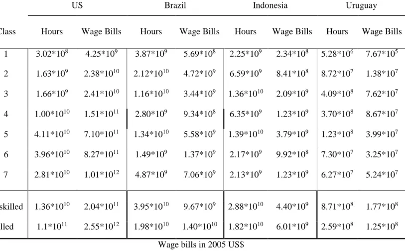
As no data set provides information on weeks worked, a figure of 49 is assumed. Aggregate labor hours will be derived by multiplying the average weekly hours worked by 49 weeks. Aggregate wage bills will be derived in a similar way, by multiplying weekly wages by 49 weeks. Table 4 provides a cross-country comparison of aggregate wage bills and labor hours for skilled and unskilled labor.

17 some university education, and the seventh comprising those with a college degree and above. We divide workers in each data set into these seven groups based on their education levels.

While most countries have similar progressions of schooling, the Brazilian school system ended its secondary education at grade 11 at the time the survey we are using was taken. To account for this, the fourth worker class in Brazil consists of workers with no more than 10 years of education, and Brazilian workers who have completed their secondary education are noted to have just 11 years of education, in contrast to the 12 years of education possessed by the fifth class of workers native to the other countries.

With the above data facilitating the construction of each country’s human capital stocks, we turn now to our Cobb-Douglas production function. Labor and physical capital stocks are taken from the Penn World Tables – allowing us to determine the per worker physical capital stock. The Penn World Tables’ RGDPe measurement gives us information on per capita income for each country in 2005 US$. Information on these measurements is provided in Table 5.

With the Penn World Tables providing data for each country’s income level and capital and labor stocks, all have only to derive each country’s human capital stock from the census data described above. Once we have found each country’s human capital stock, we will lack

information only on each country’s residual 𝐴_𝐶. This will be found simply by solving our Cobb-Douglas production function.

V. Empirical Model and Procedure Overview of our Accounting Approach

18 country’s per capita income 𝑦_𝐶, per capita capital stock 𝑘_𝐶, and the labor stocks 𝐿_𝑖,𝐶 and wage bills for each worker class. Our goal is to use this information to derive 𝐴𝐶, ℎ𝑖,𝐶, and 𝑤𝑖,𝐶 for

each country.

We begin by assuming that ℎ1,𝑈𝑆 = ℎ1,𝑐 = 1, which is equivalent to assuming that the

quality of an uneducated person’s labor is the same no matter what his nationality. This

assumption allows us to measure human capital levels for ℎ𝑖,𝐶 and ℎ𝑖,𝑈𝑆 relative to the common

base ℎ₁ = 1, and the normalization of ℎ₁ facilitates the human capital aggregation. We also normalize the skill weights µ and 𝜙, from our CES aggregators for 𝑍₁ and 𝑍₂, respectively. We do this for all countries so as to give our human capital model the “benefit of the doubt,” as it implies that cross-country income differences between workers within the same class will be due to differences in labor quality, rather than structural differences in each nation’s economy.

With these assumptions in hand, we can proceed to derive ℎ_𝑖,𝐶 by using information on the wage bill of worker class 𝑖 relative to the wage bill of worker class 1. We will show that this method produces an equation for the value of ℎ𝑖,𝐶 provided we know the substitution elasticity

between labor inputs. With the relationship between 𝑤_𝑖,𝐶, ℎ_𝑖,𝐶, 𝐿_𝑖,𝐶, and 𝑤𝑎𝑔𝑒𝑏𝑖𝑙𝑙_𝑖,𝐶 described above, we see that obtaining measurements for ℎ2,𝐶, . . . , ℎ𝑛,𝐶 easily provides measurements

for 𝑤_1,𝐶, … , 𝑤_𝑛,𝐶.

With values of 𝐻𝑖,𝐶 procured in this way, we can proceed to aggregate 𝑍1,𝐶 and 𝑍2,𝐶, in

19 Because this entire process depends on us assuming certain values for the substitution elasticity between labor inputs, we see that 𝐻_𝐶 and 𝐴_𝐶 are variables dependent on theta and epsilon. Following Jones (2014), we will show that, by assuming a relatively high level of theta, we can push down the value of epsilon such that cross-country residuals eventually reach parity.

However, our use of the term 𝑤_𝑖,𝐶 allows us to introduce a restriction that is critical to this paper: that the unobserved price of labor for any worker class in rich countries must be greater than the unobserved price of labor for any worker class in poor countries, or 𝑤𝑖,𝑈𝑆 ≥ 𝑤𝑖,𝐶.

This restriction is implied by our model, as supposing otherwise would imply that workers in rich countries should be emigrating to poor countries with relatively few educated workers, in order to cash in on those countries’ skill premiums.

Measuring Human Capital Stocks

To begin the empirical procedure, we first measure each country’s human capital stocks. We recall that the price of labor 𝑖 is given by the equation

(4) 𝑤_𝑖 = 𝛿𝑌 𝛿𝐻_𝐶

𝛿𝐻_𝐶 𝛿𝑍_1,𝐶

𝛿𝑍_1,𝐶

𝛿𝐻_𝑖 , 1 ≤ 𝑖 ≤ 𝑆

We see that the price of labor within the unskilled labor class, relative to the uneducated labor price 𝑤₁, is given by

(5) 𝑤𝑖,𝐶 𝑤_1,𝐶=

𝛿𝑍_1,𝐶 𝛿𝐻_𝑖,𝐶 ⁄ 𝛿𝑍_1,𝐶 𝛿𝐻_1,𝐶 ⁄

= (𝐻𝑖,𝐶 𝐻_1,𝐶)

𝜃−1

, 1 ≤ 𝑖 ≤ 4

Similarly, the price of labor within the skilled class relative to the least uneducated labor price 𝑤₅

is given by

(5′) 𝑤𝑗,𝐶 𝑤_5,𝐶 =

𝛿𝑍2,𝐶 𝛿𝐻_𝑗,𝐶 ⁄ 𝛿𝑍2,𝐶 𝛿𝐻5,𝐶 ⁄

= (𝐻𝑗,𝐶 𝐻_5,𝐶)

𝜃−1

20 With data on each country’s labor supply 𝐿𝑖,𝐶 and wage bills 𝑤𝑖,𝐶𝐻𝑖,𝐶, we proceed by

normalizing the quality of uneducated US laborers and the quality of uneducated foreign workers, so that ℎ_1,𝑈𝑆 = ℎ_1,𝐶 = 1. This is equivalent to assuming that the quality of an uneducated person’s labor is the same no matter what his nationality.

Finally, we normalize both skill weights in our CES equations for 𝑍_1,𝐶 and 𝑍_2,𝐶, so that µ and ϕ are equal to 1.

Having taken these steps, our unknowns remain ℎ2,𝐶, … , ℎ𝑁,𝐶 and 𝑤2,𝐶, … , 𝑤𝑁,𝐶 for all

countries. To proceed, we note that (5) and (5′) are equivalent to the equations

(6) 𝐻𝑖,𝐶𝑤𝑖,𝐶 𝐻_1,𝐶𝑤_1,𝐶 = (

𝐻_𝑖,𝐶 𝐻_1,𝐶)

𝜃

and

(6′) 𝐻𝑗,𝐶𝑤𝑗,𝐶 𝐻_5,𝐶𝑤_5,𝐶= (

𝐻𝑗,𝐶 𝐻_5,𝐶)

𝜃

Because (6) is simply the wage bill of worker class 𝑖 relative to the wage bill of uneducated workers, and because we have normalized ℎ₁ so that 𝐻₁ = 𝐿₁, we see that we can derive the capital stock of unskilled workers such that

𝐻_𝑖,𝐶 = 𝐿_1,𝐶(𝐻𝑖,𝐶𝑤𝑖,𝐶 𝐻_1,𝐶𝑤_1,𝐶)

1 𝜃 ⁄

A parallel approach allows us to calculate 𝐻_𝑗,𝐶 relative to 𝐻_5,𝐶, although it requires us to normalize ℎ_5,𝐶 and take it to be equal to one. This presents a problem, as normalizing ℎ_5,𝐶 implies that ℎ5,𝐶 = ℎ1,𝐶; however, we will compensate for this dilemma – and the fact that

21 With the capital stocks of each worker class known, their labor prices quickly follow, providing us with information on ℎ2,𝐶, … , ℎ𝑁,𝐶 and 𝑤2,𝐶, … , 𝑤𝑁,𝐶 for all countries. We can now

solve for

𝑍_1,𝐶 = 𝐶𝐸𝑆(𝐻_1,𝐶, 𝐻_2,𝐶, 𝐻_3,𝐶, 𝐻_4,𝐶; µ, 𝜃),

𝑍_2,𝐶 = 𝐶𝐸𝑆(𝐻_5,𝐶, 𝐻_6,𝐶, 𝐻_7,𝐶; 𝜙, 𝜃 ),

These equations now provide us with aggregate human capital for unskilled workers and for skilled workers, respectively.

With 𝑍_1,𝐶 and 𝑍_2,𝐶 known, we can solve for 𝐻_𝐶 = 𝐶𝐸𝑆(𝑍_1,𝐶, 𝑍_2,𝐶; 𝜌,

𝜀

process account for the fact that we have set ℎ_5,𝐶 = ℎ_1,𝐶 = 1. We have a system of two equations with three unknowns 𝐻𝑈𝑆,𝜌1, and 𝜌2:

(7) 𝐻_𝑈𝑆 = [(𝜌₁𝑍_1,𝑈𝑆)𝜀 + (𝜌₂𝑍_2,𝑈𝑆)𝜀] 1_⁄𝜀

𝜌₁+ 𝜌₂ = 1

We solve these equations for one country only, and apply whatever values have been found to the weights for all other countries as well. We do this so that differences in output will not be due to differences in the weights 𝜌₁ and 𝜌₂, but rather due to differences in human capital stocks.

We solve (7) using the US data set, and with an algebraic trick similar to (5). We see that the wage bill of unskilled workers in the US (denoted 𝑊𝐵_𝑈), divided by the wage bill of skilled workers in the US (denoted 𝑊𝐵_𝑆), is equal to

(8) ( 𝛿𝐻_𝑈𝑆

𝑍_1,𝑈𝑆 ⁄

𝛿𝐻_𝑈𝑆 𝑍_2,𝑈𝑆 ⁄

)𝑍1,𝑈𝑆 𝑍2,𝑈𝑆

= 𝜌1 𝜀_𝑍

22 This relationship between the wage bills of skilled and unskilled workers and the weights of our CES aggregator allows us to solve a system of equations equivalent to (4):

(7′) 𝜌1 𝜌₂ =

𝑍_2,𝑈𝑆 𝑍_1,𝑈𝑆(

𝑊𝐵_𝑈 𝑊𝐵_𝑆)

1 𝜀 ⁄

𝜌1+ 𝜌2 = 1

With the system of equations (7) defined, it’s clear that we have two equations and two unknowns, and hence the values of 𝜌₁ and 𝜌₂ can be found. It is also clear that the weights are dependent on both epsilon and theta. As both 𝑍_1,𝐶 and 𝑍_2,𝐶 are dependent on theta, we see that we have a clearly defined function for each country’s aggregate human capital, dependent on values of theta and epsilon:

𝐻𝐶 = [(𝜌1𝑍1,𝐶) 𝜀

+ (𝜌2𝑍2,𝐶) 𝜀

] 1_⁄𝜀

Measuring Total Factor Productivity

With information on 𝐻, and with information on each country’s capital stock K, we turn to our Cobb-Douglas production function

(9) 𝑦_𝐶= 𝑘_𝐶𝛼(𝐴_𝐶ℎ_𝐶)1−𝛼

With 𝑦_𝐶 and 𝑘_𝐶 taken from the Penn World Tables, and 𝛼 set equal to one third as is standard in the literature, we see that every term in the production function is defined for each value of theta and epsilon save for our residual 𝐴_𝐶. We remedy this by solving (9) for 𝐴_𝐶, once again giving us a variable whose value is dependent on theta and epsilon.

23 cross country income variation by the relative residual𝐴𝑈𝑆

𝐴𝐶. To facilitate our comparisons, we

create a table featuring each countries’ residual at levels of epsilon ranging from .09 to .99, reflecting a substitution elasticity between skilled and unskilled labor that ranges from approximately 1.1 to 100. We note that this is due to the relationship between the elasticity parameter in our CES model (𝜀) and the substitution elasticity between skill groups, which is defined as 1

1−𝜀.

VI. Results

Comparing cross-country levels of 𝐴𝐶, we see that when we assume the substitution

elasticity between worker classes within the same skill group is set equal to 3 (_{𝜃 = 2 3}⁄ ), human capital models become more accurate and reduce their dependence on TFP as skilled and

unskilled labor becomes increasingly inelastic. For varying levels of 𝜃, relative residuals for Brazil, Indonesia, and Uruguay all reach parity with the United States when the substitution elasticity between skilled and unskilled labor is within the range of 1.5 – 1.8. This is as expected, and supports the conclusion that accounting for inelastic labor inputs can allow human capital to account for the majority of cross-country income variation.

24 Our model was able to reduce the relative residual between the U.S. and Uruguay to 3.2 before predicting that the price of labor for workers in the sixth labor class should be higher in Uruguay than in the U.S. Our model was able to reduce the relative residual to 1.9 before predicting that the price of labor for the seventh labor class should be higher in Uruguay than in the United States. Even giving our model the benefit of the doubt and accepting 1.9 as the upper bound on our model’s accuracy, our model still over predicts Uruguay’s output by a factor of 2.

Similarly, our model was unable to reduce the relative residuals of the US and Brazil to 1 before breaking our assumption regarding the relative price of skilled labor. Our model reduced the relative residual between the U.S. and Brazil to 2.46 before predicting that the price of labor for workers in the sixth labor class should be higher in Brazil than in the U.S. Giving our model the benefit of the doubt once more and continuing, we find that our model can reduce the relative residual to 1.85 before predicting that the seventh labor class should also receive a higher price for their labor in Brazil than in the U.S. Once again, our model over predicts output by close to a factor of 2.

25 These results suggest that human capital models can indeed decrease their reliance on TFP by assuming skilled and unskilled labor are inelastic – but only to a point. As skilled and unskilled workers become more and more inelastic, the price of skilled labor in poor countries increases far more rapidly than the price of skilled labor in the United States. The result is that our model breaks our a prioriassumption long before it is able to explain the majority of cross-country income variation.

So we see that the same manipulation of elasticity parameters that can allow our model to increase its accuracy, also requires our model to predict that educated workers in rich countries should be immigrating to poor countries in order to “cash in” on high skill premiums. This contradiction suggests that we cannot manipulate elasticity parameters with abandon, and that there exists an upper bound in our model that prevents it from modeling income variation with complete (or even near) accuracy.

VII. Conclusion

In this paper, we have created a human capital model in the spirit of Jones’ generalized aggregator and derived an upper bound on the contribution of human capital to income gaps by imposing weak restrictions on skill prices. We have established that models relying on the substitution elasticity between labor inputs cannot manipulate elasticity parameters to fit an arbitrarily desired range. Instead there exists a bound on the substitution elasticity between skilled and unskilled labor that, when crossed, forces our model to confront difficult questions regarding its implications.

26 bulk of income variation by relying on a low substitution elasticity between skilled and unskilled labor, then why are skill premiums offered by countries with relatively low levels of skilled labor not enough to attract foreign professionals? What is preventing these relatively poor countries from accumulating human capital?

27 VIII. Appendix

Figure 1

Figure 1shows the relative residual (TFP) for the United States compared to Brazil, Indonesia and Uruguay. Here we have set theta to a third, representing a substitution elasticity of 3 between worker classes within each skill group. As epsilon approaches zero we see that our human capital model becomes more accurate, and correctly predicts the output of Brazil when epsilon is .17, representing a substitution elasticity of 1.2 between skilled and unskilled labor.

Note: Substitution elasticity between skilled and unskilled labor given by 1

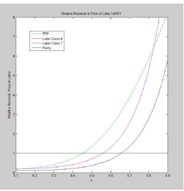
28 Figure 2

Figure 2compares the relative residual between the U.S. and Uruguay to the relative price of skilled labor between those two countries. Here the elasticity within skill groups is assumed to be 1.5. The results show that our intuition regarding the relative price of skilled labor was correct. As skilled and unskilled labor become increasingly inelastic, our model implies the existence of increasingly large skill premiums in “skill-starved” countries. Our model breaks our a piori

29 Table 1

Table1 compares the relative residual and price of labor between the U.S. and Uruguay across a range of substitution elasticity values. With this, we see that our model can explain income variation only by predicting that U.S. workers with some college education (labor class 6) or with a college, professional, or doctoral degree (labor class 7) should receive a two to threefold increase in their earnings by immigrating to Uruguay. We also see that, at its most accurate while still in line with our assumption regarding the relative price of labor, our model under predicts Uruguay’s output by a factor of 3.

Elasticity TFP Labor Class 6 Labor Class 7

1.1 0.177737 0.098537 0.188398

1.16 0.207048 0.104573 0.199938

1.23 0.248774 0.113351 0.21672

1.32 0.30864 0.126107 0.24111

1.4 0.394919 0.144647 0.276557

1.52 0.518885 0.171592 0.328074

1.64 0.694898 0.210752 0.402946

1.79 0.939722 0.267666 0.511762

1.96 1.270918 0.350382 0.66991

2.17 1.704589 0.470597 0.899754

2.44 2.253137 0.645311 1.233798

2.78 2.923703 0.899233 1.719282

3.23 3.717666 1.268271 2.42486

3.85 4.631126 1.804612 3.450314

4.76 5.656025 2.584105 4.94066

6.25 6.781504 3.716982 7.106656

9.1 7.995184 5.363451 10.25461

16.67 9.284203 7.756349 14.82969

30 Figure 3

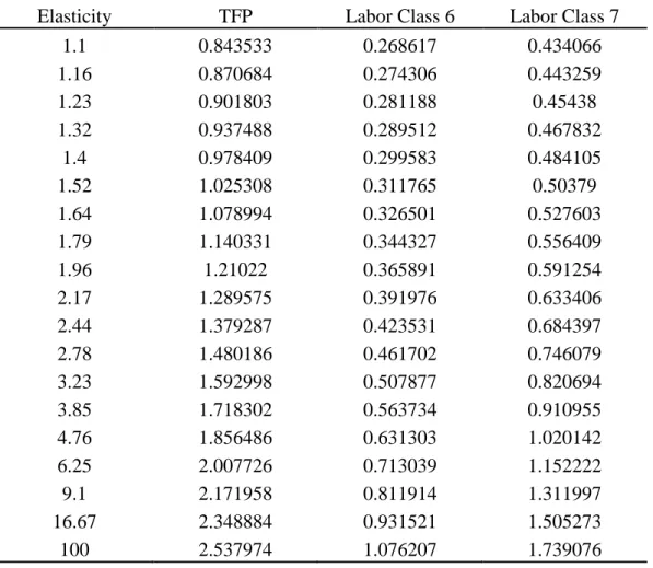
31 Table 2

Elasticity TFP Labor Class 6 Labor Class 7

1.1 0.843533 0.268617 0.434066

1.16 0.870684 0.274306 0.443259

1.23 0.901803 0.281188 0.45438

1.32 0.937488 0.289512 0.467832

1.4 0.978409 0.299583 0.484105

1.52 1.025308 0.311765 0.50379

1.64 1.078994 0.326501 0.527603

1.79 1.140331 0.344327 0.556409

1.96 1.21022 0.365891 0.591254

2.17 1.289575 0.391976 0.633406

2.44 1.379287 0.423531 0.684397

2.78 1.480186 0.461702 0.746079

3.23 1.592998 0.507877 0.820694

3.85 1.718302 0.563734 0.910955

4.76 1.856486 0.631303 1.020142

6.25 2.007726 0.713039 1.152222

9.1 2.171958 0.811914 1.311997

16.67 2.348884 0.931521 1.505273

100 2.537974 1.076207 1.739076

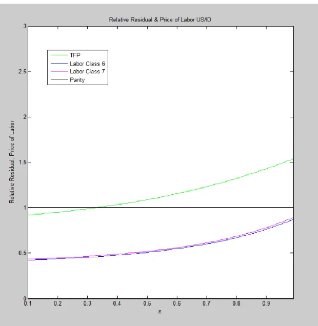
32 Figure 4

Figure 4compares the relative residual between the U.S. and Indonesia to the relative price of

skilled labor between those two countries. Here the inner elasticity is set equal to5

3. We see that

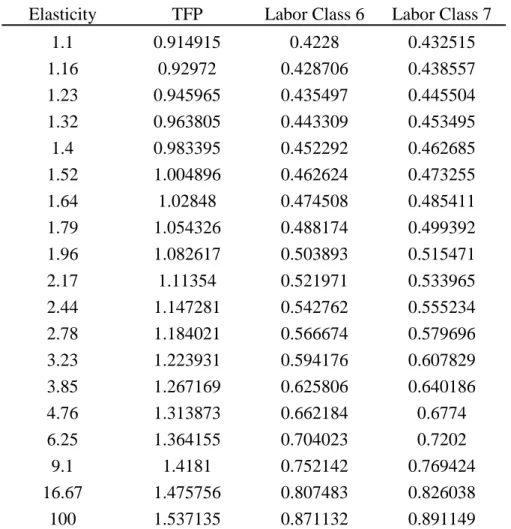
33 Table 3

Elasticity TFP Labor Class 6 Labor Class 7

1.1 0.914915 0.4228 0.432515

1.16 0.92972 0.428706 0.438557

1.23 0.945965 0.435497 0.445504

1.32 0.963805 0.443309 0.453495

1.4 0.983395 0.452292 0.462685

1.52 1.004896 0.462624 0.473255

1.64 1.02848 0.474508 0.485411

1.79 1.054326 0.488174 0.499392

1.96 1.082617 0.503893 0.515471

2.17 1.11354 0.521971 0.533965

2.44 1.147281 0.542762 0.555234

2.78 1.184021 0.566674 0.579696

3.23 1.223931 0.594176 0.607829

3.85 1.267169 0.625806 0.640186

4.76 1.313873 0.662184 0.6774

6.25 1.364155 0.704023 0.7202

9.1 1.4181 0.752142 0.769424

16.67 1.475756 0.807483 0.826038

100 1.537135 0.871132 0.891149

Table 3compares the relative residual and price of labor between the U.S. and Indonesia across a range of substitution elasticity values. Our model can explain income variation only by

34 Table 4

Table 5 compares aggregate labor hours and wage bills for each labor class across countries, as accounted for in our IPUMS datasets. This highlights the relative scarcity of skilled labor in poor countries compared to the U.S. The aggregate labor hours of college educated workers in the U.S. is 100 times greater than the aggregate labor hours of workers with no education. Overall, skilled labor in the U.S. is almost ten times as plentiful as is unskilled labor. In Brazil and Indonesia, workers who have not completed primary school produce five times as many labor hours as college educated workers, and aggregate unskilled labor hours are more than three times as large as aggregate skilled labor hours in Uruguay.

US Brazil Indonesia Uruguay

Class Hours Wage Bills Hours Wage Bills Hours Wage Bills Hours Wage Bills 1 3.02*108 4.25*109 3.87*109 5.69*108 2.25*109 2.34*108 5.28*106 7.67*105 2 1.63*109 2.38*1010 2.12*1010 4.72*109 6.59*109 8.41*108 8.72*107 1.38*107 3 1.66*109 _2.41*1010 _1.16*1010 _3.44*109 _1.36*1010 _2.09*109 _4.09*108 _7.62*107 4 1.00*1010 1.51*1011 2.80*109 9.34*108 6.35*109 1.23*109 3.70*108 8.67*107 5 4.11*1010 7.10*1011 1.34*1010 5.58*109 1.39*1010 3.79*109 1.23*108 3.99*107 6 3.96*1010 8.27*1011 1.49*109 1.37*109 2.17*109 9.92*108 7.30*107 3.25*107 7 2.81*1010 1.01*1012 4.87*109 7.06*109 2.13*109 1.23*109 6.27*107 5.24*107

Unskilled 1.36*1010 2.04*1011 3.95*1010 9.67*109 2.88*1010 4.40*109 8.71*108 1.77*108 Skilled 1.1*1011 2.55*1012 1.98*1010 1.40*1010 1.82*1010 6.01*109 2.59*108 1.25*108

35 Table 5

Measure U.S. Brazil Indonesia Uruguay

Panel A: Accounting Measurements

Real GDP

(mil. 2005 US$) 10711100 1146806 512643.3 28369.6

𝑦_𝑈𝑆 𝑦_𝐶

⁄ _{1 5.058204 12.94489 3.114636}

Capital Stock

(mil. 2005 US$) 28316298 3622159 831277.3 106252.8

𝑘_𝑈𝑆 𝑘_𝐶

⁄ _{1 4.233712 21.10426 2.198479}

Persons Engaged (mil.) 136.3844 73.8613 84.4976 1.1251

𝐿_𝑈𝑆 𝐿_𝐶

⁄ _{1 1.846493 1.614062 121.2198}

Panel B: TFP’s Contribution to Income Gaps

𝐴_𝑈𝑆 𝐴_𝐶 ⁄

(𝑤_6,𝑈𝑆 ≤ 𝑤_6,𝐶) 1 2.46 1.53 3.1

𝐴_𝑈𝑆 𝐴_𝐶 ⁄

(𝑤_7,𝑈𝑆 ≤ 𝑤_7,𝐶) 1 1.83 1.53 1.85

Lower case variables denote per worker measurements.

36 Table 6

Variable Description U.S. Brazil Indonesia Uruguay

age Age of respondent 39.9 35.2 34.67 39.1

classwk

Field respondent works in. This variable includes local and federal government, private (nongovernment) for profit and not for profit firms, and domestic labor

(0 = “private sector firm for wages”) 0 0 0 0

HRSWRK1 Number of hours worked per week. 43.58 47.67 47.88 N/A

incwage Wage income. 37357 N/A 219430 6080.48

incself Income earned as independent business owner. 0 0 0 0

incearn Earned income 37328 565.92 N/A N/A

school Whether respondent is currently in school. (0 = “No”) 0 0 0 0

wrkmths Months worked in the past year. 11.38 N/A N/A N/A

yrimm Year immigrated. (0 = “Not immigrant”) 0 N/A N/A N/A

educus Highest education level attained.

Some

College N/A N/A N/A

edattan Highest education level attained. Secondary Primary Primary Primary

yrschl Number of years of schooling. N/A 7.08 9.06 8.46

nativty Respondent's country of birth (0 = “Native”). 0 0 0 0

hrsmain Hours per week worked in main job. N/A 46.87 47.29 48.67

37 Works Cited

Alan Heston, Robert Summers and Bettina Aten, Penn World Table Version 7.1, Center for International Comparisons of Production, Income and Prices at the University of Pennsylvania, Nov 2012.

Bowlus, Audra J., and Chris Robinson. "Human Capital Prices, Productivity, and Growth."

American Economic Review 102.7 (2012): 3483-515. Web.

Caselli, Francesco. “Accounting for Cross-Country Income Differences,” The Handbook of Economic Growth Aghion and Durlaug eds., Elsevier, 2005

Caselli, Francesco. "The World Technology Frontier." The American Economic Review 96.3 (2006): 499-522. Web.

Feenstra, Robert C., Robert Inklaar and Marcel P. Timmer (2013), "The Next Generation of the Penn World Table" available for download at www.ggdc.net/pwt

Hendricks, Lutz. "How Important Is Human Capital for Development? Evidence from Immigrant Earnings." American Economic Review 92.1 (2002): 198-219

Jones, Benjamin F. “The Human Capital Stock: A Generalized Approach.” American Economic

Review. Forthcoming 2014.

Matthew Sobek, Steven Ruggles, Robert McCaa, et al., Integrated Public Use Microdata Series- International: Preliminary Version 0.1 Minneapolis: Minnesota Population Center University of Minnesota, 2002