The Scheduling of Controversial Roll-Call Votes in State Senates By
Grace Garner
Senior Honors Thesis Political Science
University of North Carolina at Chapel Hill
3/27/18
Approved:
Abstract
In the US Congress it has been shown that factors such as the electoral cycle, seat stability, and party strength affect how legislators approach dealing with legislation, especially potentially controversial legislation. I believe that there remains much to be gained from analyzing state senates and deriving patterns in roll-call voting behavior. I examine the
Introduction
The roll-call voting patterns of US Congress legislators have been the subject of many studies, particularly in the senate. Understanding common legislator behavior factors directly into understanding how the government functions on a practical level, answering questions such as: Why do legislators sometimes vote one way, and then a few years later vote the other way? What factors, other than personal beliefs, influence legislators to vote one way or another? What factors influence when and on what sort of legislation legislators vote? This last question is the focus of this study.
The literature review summarizes the patterns that are well-established in the US Congress and outlines the limited knowledge about patterns at the state level. The desire to be re-elected is shown to influence individual legislators’ voting behavior, and these behavioral changes are
patterned according to the length of the election cycle and at what point in the election cycle the vote takes place, as well as the makeup of the constituency and the party membership of the legislator. This effect holds true and even becomes more pronounced for controversial legislation. There is very limited scholarship on state legislator behavior. The studies that do exist suggest that state legislators do not vary their behavior as much, but these are inconclusive at best.
Studying state legislators as a group is complex, as state legislators are working in fifty different environments. These varying environments make it difficult to account for all of the potential confounding variables. To simplify matters as much as possible, I limit my study to state senates and legislation involving the expansion or restriction of abortion access. The main issue was that I wanted to find a general pattern that could potentially fit all, or most state senates. And so, I create a design that accounts for many of the differences between state legislative bodies, avoiding confounding variables. I also used the scheduling of the roll-call votes as my main units of analysis: or, when in the election cycle roll-call votes were placed on each senate’s calendar. To further account for differences, the analysis of the different pieces of
legislation comes in three phases, only the last of which deals with the actual roll-call vote itself. The research design section will outline the data that was gathered, the methods by which it was gathered, and how it was processed and analyzed.
The last section will cover the results of the analysis and summarize the findings.
Literature Review
The studies examined here and the design and analysis following operate on the assumption that all elected officials desire to be re-elected and much of their behavior will be influenced by that desire, as outlined by Mayhew (1974).
their previous election. It was assumed that the winners of these elections won “randomly,” as
the election could have easily been swayed if a few more constituents had decided to vote that day. These “random assignment” electoral win districts are then compared to other districts, where the “probability” of being re-elected is calculated according to whether the party had previous wins in these districts. It stands to reason that the “randomly-assigned” winners would
have a smaller probability of being re-elected than winners of other districts, and thus would likely be more concerned with pleasing their constituents. Looking at the voting records of the “randomly assigned” winners and the voting records of the legislators with a high probability of
being re-elected, they found that their voting records were very similar, suggesting that either the legislators are not concerned at all about the effects of their roll-call votes on their prospects of being re-elected (unlikely), or (more likely), US House members are very concerned with
establishing a consistent voting record because they must run for re-election so often. It stands to reason then that the US House legislators tend to consistently vote as their constituency would expect, regardless of their probability of being re-elected.
In their 1978 study Amacher, Ryan, and Boyes ran an analysis of the roll-call voting behaviors of US Senators on the premise that the length of the election cycle affects how independently US senators feel they can operate without jeopardizing their chances of re-election. They measured the differences between US Senate legislators’ roll call votes and US House legislators’ roll call votes within a certain time period – in this case, the 93rd Congress.
Under the assumption that the US House legislators’ roll call voting behavior more closely matched the desires of a state’s constituency, they measured by how much senators deviated
facing re-election) voted much more independently than those near the end of their election cycle (one or two years away from facing re-election).
The results of these two studies establish that the length of an election cycle has an effect on the roll-call voting patterns of US legislators, and it is this fact that convinced me to limit my study to state senates. The varying election cycle types of state senates allow me to study how different election cycles may affect the scheduling of roll-call votes.
Moreover, a study of influences on US Senators by John Jackson in 1974 found that constituencies’ opinions affected senatorial voting behavior more so than other significant
influences, such as political parties, committee leaders, the President, or other leaders. A study by Steven Levitt in 1996 looked at this in more detail by tabulating how senators “weigh” the
various influences around them when considering how to vote, including their own ideology and the preferences of their constituency. He found that while senators always consider to some extent the preferences of their constituency, they more heavily weigh their constituency
preferences as an election approaches. In other words, they give more consideration to what their constituents want as they are coming up for re-election. This fits with the assumption that
senators (and elected officials in general) desire to be re-elected, and will modify their behaviors to something more desirable for their constituents, when those constituents are more likely to be paying attention. This is another basis for my study: I assume that senators will schedule roll-call votes depending on whether they want their constituents to be paying attention, or whether they’d prefer their roll-call votes to be more hidden.
abortion) and analyze by how much US senators were motivated beyond their own ideology to cast certain roll call votes. They looked specifically at senators where their “party ideology” (an assumed measure of their personal ideology) doesn’t match up with their “state ideology”—eg, a
pro-life Republican from a pro-choice state. They found that senators who had to face many different sorts of constituents (eg, a pro-life Republican facing a pro-life constituency in a primary election but a pro-choice constituency in the general election) had different voting patterns on the issue of abortion than senators with a more homogenous constituency (eg, a pro-life Republican from pro-pro-life Texas). This suggests that the preferences of constituencies play a role in influencing the roll-call votes of senators, even when they disagree with their senator’s party, and even in the case of issues with strong ideological connotations.
Though these behavioral tendencies are fairly well-established at the federal level, they are less so at the state level. There are fewer studies that attempt to study state legislator behavior – partially because the state level can get more complex. Those that do study state legislator
behavior have not found strong indications one way or the other on how the electoral cycle may or may not affect legislator roll-call voting behavior. Steven Rogers’ 2017 study looks at public opinion on key roll call votes, how the legislators voted, and the subsequent effect on the legislators’ vote share in the following election. He was unable to find any correlation between
ideologically constant. Like Rogers’ study, this suggests that state legislators don’t have the same concerns that federal legislators do regarding re-electability.
Theory
There are several broad conclusions we can draw from the literature: first, that the length and type of election cycle is an important factor in understanding the roll-call voting behavior of legislators. Second, that the closer a vote takes place to an election, the more likely senators are to vote according to what their constituents would want – and conversely, the further away a vote takes place to an election, the more likely senators are to vote against what their constituents would want. These two facts together suggest that when in the election cycle a vote takes place is an important predictor of how senators may vote. Third, controversial roll-call votes carry with them more weight and risk than regular votes. Research on state senators’ behavior shows a
greater tendency to stay ideologically consistent and not be as strongly influenced by their constituencies in comparison to their federal counterparts. However, this information has been pulled from a large pool of senatorial roll-call votes, regarding all types of legislation. When certain types of legislation are isolated, a pattern may emerge. It’s reasonable to theorize that
roll-call vote patterns with controversial legislation may be more pronounced than other votes, as they may get much riskier nearer to an election than other types of roll-call votes. It is for this reason that I decided to use abortion legislation as the focus of this study – it is a very
Because there is only one body of interest in federal studies of senators (the US Senate), the units of analysis are typically individual votes by individual senators, analyzed over time. Usually, the intent is to examine in one way or another how individual senators believe their roll-call votes may affect their re-election prospects. Unlike in studies at the federal level, recording how individual senators’ voting patterns change over time is not feasible at the state level.
Because individual state senators are in varying environments from state to state, there are innumerable differences between each seat in each senate in each state. For practical purposes then, my intent is so find general trends in state senates for scheduling controversial roll-call votes, rather than general trends for state senators’ roll-call voting behaviors. If senators of a
party believe a certain controversial roll-call vote may damage their re-election prospects, it is reasonable to hypothesize that they are more likely to attempt to schedule it earlier in the election cycle, and vice versa.
When studying state senates, we have the ability to exploit a natural experiment –
The election cycle is the predominate subject of interest in this study. If state senators are concerned about how their behavior surrounding the abortion issue may influence their base of support in their district in their next election, then they will modify their behavior in order to benefit their next election. This desire is the same at the party level – the Republican Party will generally work as a unit to get as many Republican senators re-elected, and the same goes for the Democratic Party. What I am examining is the timing of scheduled roll-call votes and observing subtle changes in the schedule that legislators may use to benefit their upcoming elections.
I hypothesize that a weaker party will be motivated to take risks in the hope that they can gain some political ground, and so will attempt to schedule controversial votes later in the election cycle so as to “rock the boat” and motivate their base to vote on Election Day.
Conversely, a strong party has no motivation to “rock the boat” and risk losing support and so
will try to have controversial votes scheduled earlier in the election cycle, when the electorate is less likely to be paying attention and more likely to forget anything that offends them by Election Day.
As demonstrated at the federal level, the shorter election cycles of the US Congress don’t
allow for enough temporal “wiggle room” for legislators to change their behaviors drastically. Therefore, I expect that a longer election cycle will allow for more variation in scheduling than in shorter or staggered election cycles.
State Senates also vary in their levels of professionalism. This is likely to influence both how concerned they are with re-election and how much influence controversial legislation has over that re-election.
Hypothesis 1: A stronger party (as defined in subheadings a – d) will schedule
controversial votes earlier in the election cycle. A weaker party will schedule controversial votes later in the election cycle.
a. Average vote share per seat – indicative of the party’s average control of individual seats
b. Average seat gain or loss per election cycle – indicative of party’s climbing or declining strength over the period of years of interest
c. Recent control change – indicative of how precarious a party’s control of Congress is
d. Party control – indicative of whether a party controls over 60% of the seats or not when a bill is proposed
Hypothesis 2: Longer election cycles will have more evident patterns than shorter election cycles and election cycles with staggering
Hypothesis 3: More professional Senates will have more evident patterns in scheduled votes than less professional Senates.
Data and Methods
are upcoming, which increases the probability that senatorial behaviors will change throughout the election cycle.
The years in which I gathered legislation data range from 2010-2016, with a majority within the years 2012-2016, depending on when the election cycles took place. I wanted the timing to be relatively recent and with relatively constant national conditions – therefore a time with a single president and arguably no dramatic changes that affected the entire country, like the 2008 economic crash.
In order for a piece of legislation to be put up for a vote, it must first be put through a vetting process. In order to reasonably compare voting patterns in different states, the differences in the likelihood of a piece of abortion legislation to even make it to the voting stage must be
established. To do this we will run data on pieces of abortion legislation through three stages.
Stage 1. Whether the relevant legislation is proposed
o Do senators even attempt to bring up controversial legislation?
o For some Senators (for example, those in the minority party), bringing up
controversial legislation may be too big of a risk: their re-election strategy may be to make no trouble. For states where this is the case, obviously there will be no roll-call votes for controversial legislation. This stage will filter these states out. Stage 2. Whether the proposed legislation is scheduled for a roll-call vote
o Under what circumstances is a vote scheduled?
o In many states, especially those when the opposing party is in power or when
Congress but then shunted off to a committee where it dies and is never brought to the floor for a roll-call vote.
Stage 3. When in the election cycle the roll-call vote takes place
o Do re-election concerns affect when roll-call votes on controversial legislation
take place?
o The primary question: when the conditions allow for bringing controversial
legislation to a roll-call vote, when do the parties schedule the vote?
Dependent Variable/Units of Analysis
The data on abortion legislation was gathered by hand, using primarily state senate website records, where every piece of legislation proposed and any votes or extraneous
information about the legislation is archived by session. Occasionally, a state website would only have part of the information I needed (eg, just the legislation summary and not the full text, or no voting records). When this problem arose I supplemented the gap through the use of the website Legiscan. These two sources in tandem allowed me compile all the information I needed.
The following criteria were used in the selection of abortion legislation. Specific limits were imposed in order to prevent any confusion or blurred lines about the possible intention behind the legislation.
A bill is included in the analysis when it expands or restricts abortion access: eg, limits who can receive an abortion, when they can receive an abortion, or produces a more convoluted process for receiving abortions (longer wait times, etc.). This includes codifications and
There are also certain common types of legislation that I am NOT including despite their potential connections with abortion, for specific reasons. These are:
Chemical abortion regulations. This is still a fairly new area of medicine, and as
such it’s natural that new regulations are still being introduced. It’s impossible to
tell which ones are intended to restrict access and which ones are simply providing a framework in which providers can work with this new technology. Telehealth regulations, for the same reasoning as above
Anti-coercion laws: this is not restricting access, but providing safety from
potential abuse.
Conscience laws (eg. providing medical personnel with the right to refuse to
perform abortions). This does not in any significant way prevent abortion-seekers from having access to these services.
Birth control laws
Amendments/laws classifying certain actions (that are already illegal), or spelling
out the punishment (eg., classifying partial-birth abortion as a felony)
Amendments whose purpose are to clarify that certain services do not include
abortions
An important note: In the process of gathering this data, eight states were eliminated from the analysis for one of the following three reasons.
1. There simply is no data to be found (there are no relevant pieces of legislation): Alaska, Connecticut, Montana, Nevada, North Carolina, Wyoming
specifically 2011-2013-2017. Because I was only analyzing the 48-month patterns with these types of cycles, New Jersey simply didn’t have a 48-month block that I
could use.
3. Nebraska is unicameral.
Independent Variables
The independent variables of interest were gathered and analyzed as follows.
1. Strength of political parties
a. Average vote share per seat – Intended to measure the average safety of
individual seats. Election data was gathered for each state in a single election. The percent of the vote gathered for the Democratic Party and the Republican Party were calculated for each seat up for re-election, and then averaged. 2012 was used when possible, but for the handful of states that didn’t have elections that year,
2011 or 2014 were used instead.
i. Continuous variable ranging from 0 to 1.
b. Average %seat gain or loss per election cycle – Intended to measure a party’s growing or declining strength over the period of interest. Because legislation data was gathered over the years 2010-2016, I looked at election data for the years 2009-2016. Over that period of years, I calculated the average number of seats gained or loss per the number of elections had by each state.
c. Recent control change – Intended to measure how “solid” a party’s control of the senate is. For each state, I selected the election year that begins the period in which I gathered data for that state (2010, 2011, or 2012, with most being 2012) and looked to see if party control changed in that election. I measured “change”
by calculating whether one party controlled at least 60% of the seats in the senate and if that control was gained or lost in that election. (E.g., if neither party had a 60% majority before the election and one gained it during the election it is coded as a control change.)
i. Dummy variable: 0 for no change, 1 for change
d. Party control – Intended to measure a party’s control when a piece of legislation is introduced. A “party controlled” senate will have 60% or greater of its seats
controlled by that party.
i. -1 = Democrat controlled, 1 = Republican controlled, 0 = neither 2. Election cycle lengths/type
a. Taken from common knowledge: election cycles are categorized by their length as measured by months (48, 24-48-48, 24) and the cycle type is either staggered or non-staggered. For simplicity, the 24-month cycles are treated as 48-month cycles, with data only gathered from one of the 48-48-month-cycle periods.
i. Non-staggered 48-month cycles are coded as 1, staggered 48-month cycles are coded as 2, and 24-month cycles are coded as 3.
3. Senate professionalism
legislators spend on the job, the amount they are compensated, and the size of the legislator’s staff. The original analysis was completed in 2008, and I’m making
the assumption that if analyzed again (for the year 2012, for example) the professionalism levels of the senates would not have changed significantly.
i. I took the color-coded categories and assigned integers ranging from -2 (unprofessional) to +2 (very professional).
The dependent variables vary by Phase. Phase 1
o Binary variable: proposal present/not present (1,0) o Logistic regression
Phase 2
o Binary variable
DV: roll-call vote present/not present (1, 0)
IV: cycle_type, timing_proposal, professionalism, party_security Party security: control_change, avg_vote_share,
avg_seat_loss_per_election o Logistic regression
Phase 3
o Continuous variable from 0 to 1, the timing of roll-call votes given on individual
controversial pieces of legislation
DV: roll-call vote present/not present (1, 0)
Party security: control_change, avg_vote_share,
avt_seat_loss_per_election
o I first look up the beginning and ending election cycle dates for each state in the
relevant time period (eg, 11/4/10 – 11/6/14). Each month within that time period (count them: 48) is assigned a number. November 2010 is #1, December 2010 is #2, January 2011 is #3, etc. I then look up the date for the first relevant roll-call vote given on each piece of relevant legislation in that state in the relevant time period. For example, 4/15/2011. April of 2011 is month #6 (six months since the last election). 6/48 = 0.125. The closer to 1 this number is, the closer to the following election that vote takes place.
o The first non-procedural roll-call vote is used o Linear regression
o Previous state legislatures never hold a session after an election date, so there is no risk of “spillover.”
Analysis
Stage 1
The intent of Stage 1 of the analysis is to draw broad conclusions as to why certain states proposed abortion legislation while others did not.
statistical analysis other than simple summary statistics because there were so few states that had no data points.
One thing that all six had in common was there was no recent party control change, compared to about 30% of the other states with data that did have recent control change. They were also spread out geographically and were varied in their party control: North Carolina and Wyoming had Republican-controlled Senates, Connecticut had Democrat-controlled Senates, Montana and Nevada had neither party in control, and Alaska changed in 2012 from neither having control to Republicans having control. Their election cycle type, percent of Republican seats gained or lost per election, average Republican vote share per seat, and level of
professionalism were similarly varied. From this information, we can hypothesize that perhaps the Republican and Democrat party-controlled senates felt stable as there had been no recent power change, and thus weren’t willing to bring up controversial subjects and risk upsetting the
status-quo. This doesn’t explain why Montana and Nevada didn’t bring up controversial subjects, unless they were perhaps afraid of losing what ground they had gained.
away from controversial legislation when they are weaker and striving for a majority. Or, it could simply mean that without control of the senate, they know it’s not likely that their
proposed legislation will come to a roll-call vote, and so don’t bother.
In short, there is no clear reasoning for why these handful of states had no relevant data.
Stage 2
The intent of Stage 2 is to determine under what conditions abortion legislation that has been proposed is scheduled for a roll-call vote.
I first tested all independent variables separately. I also took note of the different sorts of abortion legislation under consideration. There are two main varieties – the expansion and the restriction of abortion access. I created a restriction dataset from the legislation that contained only legislation for the restriction of abortion access. Because the majority of data I gathered had to do with restrictive abortion legislation, a dataset containing only expansion legislation would have been much smaller than either of the others (36 datapoints), and so I didn’t test with it.
Similarly, the opposite of other datasets (i.e., an “unprofessional” dataset) didn’t have a good fit and so weren’t included. Recall that Hypotheses 2 and 3 are that more professional senates and
senates with longer, non-staggered election cycles will have more distinct patterns. From the complete dataset and the restriction dataset then I created six datasets in total.
Table 1: Datasets
Dataset Title Data Contained in Dataset Data points
Complete All data 229
Restricted Abortion restriction data only 193
Professional Most professional senates (0 – 2) only 172 Professional+Restriction Most professional senates (0 – 2) only,
abortion restriction data only
Cycle+Restriction 48-month non-staggered election cycles only, abortion restriction data only
84
I ran every model in Stages 2 and 3 with each dataset to watch for unexpected
differences. However, because of the partisan split between the restriction of abortion access and the expansion of abortion access I only discuss the results of the restricted dataset when running models with independent variables that are party-specific, unless an unexpected difference appears between datasets. Additionally, I only show the R output when there appeared to be a relationship. For a single model, if there are relevant differences in the results of different datasets, I show and discuss the results of each.
All modeling was done using R.
The following binomial models for Stage 2 were created as follows.
Table 2: Binomial Regression Models Model X Value
(Categorical)
Y Value Dataset Emphasis Results Summary Model
1
Cycle type (months) 1: 48
2: 48 (staggered) 3: 24 Presence of RC Vote Complete Professional Cycle n/a Model 2 Professionalism -2: Unprofessional 2: Professional Presence of RC Vote Complete Professional Cycle More professionalism, less likely to be a vote
Model 3
Recent Control Change
0: No recent change 1: Recent change
Presence of RC Vote
All six n/a
Model 4
Party Control
-1: Democratic control 0: Neither control 1: Republican control
Presence of RC Vote Restriction Professional+Restriction Cycle+Restriction Strong Republican party, more likely to be a vote Model X Value
(Continuous)
Y Value Dataset Emphasis Results Summary Model
5
%Seat Loss/Gain Ranging from -1 to 1
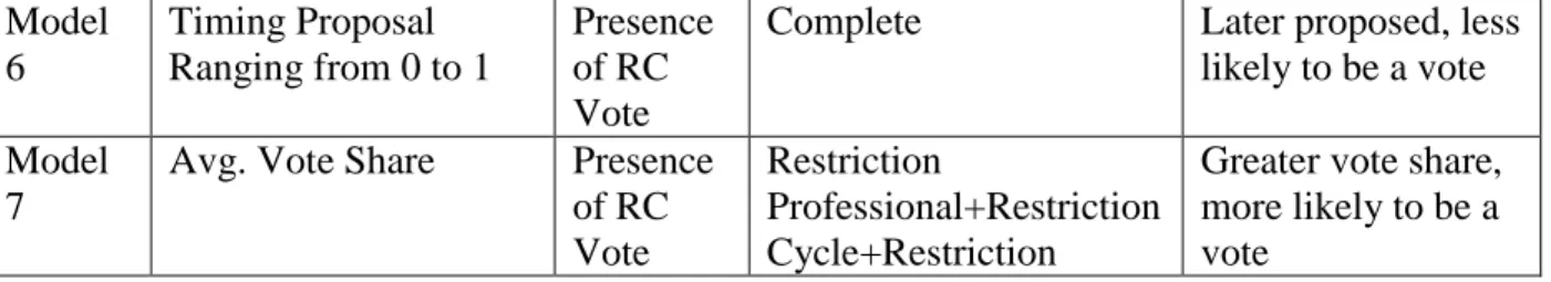
Model 6
Timing Proposal Ranging from 0 to 1
Presence of RC Vote
Complete Later proposed, less likely to be a vote Model
7
Avg. Vote Share Presence of RC Vote
Restriction
Professional+Restriction Cycle+Restriction
Greater vote share, more likely to be a vote
The residual deviances on all models were large, but of these first seven, models 2, 4, 5, 6, and 7 showed a small amount of fit. The results gained from the two basic datasets (complete and restriction) did not differ from the other, smaller datasets used to test the models, so only the complete and restricted dataset results will be shown.
I analyzed Model 2 with the complete dataset because professionalism is not party-specific. The complete dataset had a slightly better fit than the restriction dataset anyway, which is understandable because it and has a wider variety of variables that the restricted dataset. The results of running Model 2, seen in Table 3, suggest that the more professional a senate is, the less likely it is for abortion legislation to come to a roll call vote. This could be because a more professional senate has greater re-election concerns, and thus the senators and their parties are more cautious and less willing to broach controversial subjects.
Table 3: Professionalism (complete) Professionalism Coefficient
(standard error)
-2 1.099
(1.155)
-1 -2.223.
(1.198)
0 -2.485*
(1.176)
1 -2.197.
(1.291)
2 -3.008*
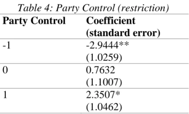
Model 4, contrary to Model 2, has the party-specific variable of party control (more than 60% of seats controlled by a single party). It’s reasonable to assume that different types of abortion legislation would be treated differently depending on whether its “favorable” party
controls the senate or not; restrictive abortion legislation will theoretically be treated differently under a Democrat-controlled senate than under a Republican-controlled senate. The results of running Model 4, seen in Table 4, suggest that roll call votes of restrictive abortion legislation are more likely to occur under a strong Republican party. This is unsurprising, since it’s easy for
legislation to die in committee when their favored party is not in control of the senate.
Table 4: Party Control (restriction) Party Control Coefficient
(standard error)
-1 -2.9444**
(1.0259)
0 0.7632
(1.1007)
1 2.3507*
(1.0462)
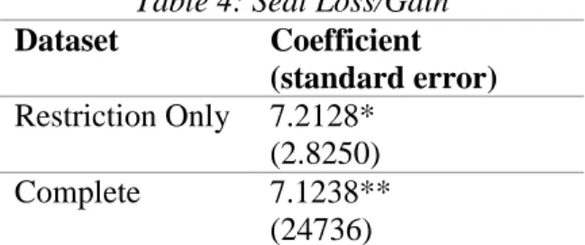
Model 5, similar to Model 4, had a variable that was party-specific. Percentage of seat loss/gain refers to the Republican Party only. A negative value indicates Republican seat losses, a positive value indicates Republican seat gains. Again, I ran both the complete and restricted datasets. The restricted set had a larger standard error, but is likely more accurate (Table 4). However, even with the complete dataset (Table 4), the results were similar: the more seats the Republican Party gained on average, the more likely a vote would be scheduled. This is
be coincidental. However, it could also imply that political parties don’t necessarily employ
different methods for different types of legislation in regards to scheduling roll-call votes. The complete dataset results imply that when Republicans gain more seats, they are more likely to schedule roll-call votes regardless of whether they are for pro-life legislation or for pro-choice legislation, which goes against what I would expect, as I’ve assumed that a
Republican-controlled senate would leave pro-choice legislation in committees to die.
Table 4: Seat Loss/Gain Dataset Coefficient
(standard error) Restriction Only 7.2128*
(2.8250) Complete 7.1238**
(24736)
Model 6 had variables that were not party-specific, so I used the results from the complete dataset. The “proposal timing” variable is of particular interest, because it has to do
with when certain actions take place in the election cycle. The results show that the later a piece of legislation is proposed, the less likely it is for that same piece of legislation to be scheduled for a roll-call vote (Table 5). This could suggest a general trend towards caution: it may be that senators would generally prefer to schedule controversial votes earlier in the election cycle, regardless of the current strength or weakness of their party.
Table 5: Timing Proposal (complete) Variable Coefficient
(standard error) Timing Proposal -1.4145*
(0.6759)
percentage of the vote share that the Republican Party receives, the more likely it is for a roll-call vote to be scheduled. This makes sense because a strong party makes it easier for proposed legislation to be scheduled, rather than shunted off to die somewhere in committee.
Table 6: (restriction) Variable Coefficient
(standard error) Avg. Vote Share 4.296*
(1.815) Stage 3
The intent of Stage 3 is to determine what factors influence when a roll-call vote is scheduled. This can be considered the highlight of this study. As in Stage 2, I used all six
datasets when attempting to find patterns. After examining each variable independently, I created multiple linear regressions and found some more distinct patterns within those.
The models for Stage 3 were as follows.
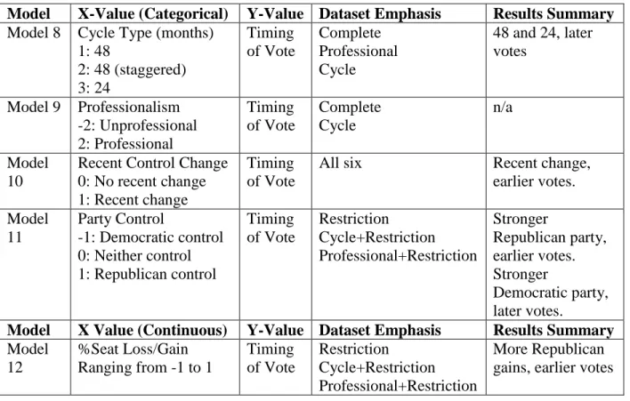
Model X-Value (Categorical) Y-Value Dataset Emphasis Results Summary Model 8 Cycle Type (months)
1: 48
2: 48 (staggered) 3: 24 Timing of Vote Complete Professional Cycle
48 and 24, later votes
Model 9 Professionalism -2: Unprofessional 2: Professional Timing of Vote Complete Cycle n/a Model 10
Recent Control Change 0: No recent change 1: Recent change
Timing of Vote
All six Recent change,
earlier votes. Model
11
Party Control
-1: Democratic control 0: Neither control 1: Republican control
Timing of Vote Restriction Cycle+Restriction Professional+Restriction Stronger Republican party, earlier votes. Stronger Democratic party, later votes.
Model X Value (Continuous) Y-Value Dataset Emphasis Results Summary Model
12
%Seat Loss/Gain Ranging from -1 to 1
Model 13
Timing Proposal Ranging from 0 to 1
Timing of Vote
Complete Later proposal,
later votes Model
14
Avg Vote Share Timing of Vote
Restriction
Cycle+Restriction Professional+Restriction
Greater vote share, earlier votes Table 7: Linear Regression Models
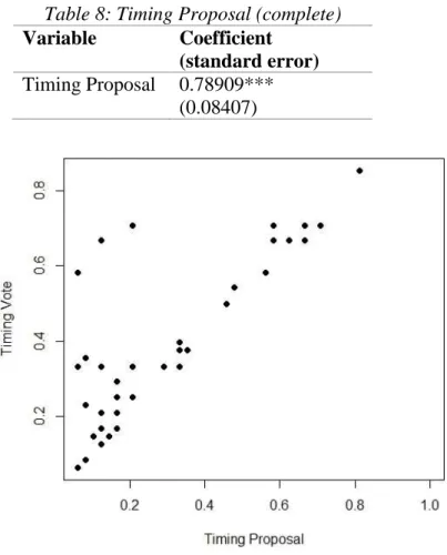
As with the binomial regressions, almost all of the linear regressions had poor R2 values on their own. The exception was Model 13, but the reason is obvious: when a roll-call vote is scheduled is understandably closely related to when it was first proposed (Table 8).
Table 8: Timing Proposal (complete) Variable Coefficient
(standard error) Timing Proposal 0.78909***
(0.08407)
Figure 1 - Scatterplot, Timing Vote vs Timing Proposal
the models were improved as well by use of the other datasets. Models 8, 10, 11, 12, 13 (already shown in Table 8), and 14 all appeared to have some correlation between the variables.
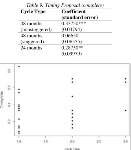
Model 8 was the only model that did best with the simple complete dataset. Cycle types are not a party-specific variable, and so the complete dataset results are presented in Table 9. They suggest that cycle types consisting of 48 non-staggered months and 24 months had roll-call votes scheduled later in the cycle. This is an interesting potential relationship, since I can’t see
any immediate reason for why this would be. The R2 is extremely small however, so it’s possibly just coincidental.
Table 9: Timing Proposal (complete) Cycle Type Coefficient
(standard error) 48 months
(nonstaggered)
0.33750*** (0.04794) 48 months
(staggered)
0.06650 (0.06555) 24 months 0.28750**
(0.09979)
Figure 2 - Scatterplot, Model 8, Timing Vote vs Cycle Type (complete dataset)
The Model 10 results were most evident with the professional and
one taken from professional as its data had the greatest variety (Table 9). The results indicate that roll-call votes take place earlier in an election cycle when there has been a recent control change, and take place later when there has been no control change. This potentially runs contrary to my Hypothesis 1, which stated that stronger parties will schedule roll-call votes earlier in an election cycle, and weaker parties will schedule roll-call votes later in an election cycle. In theory, a recent control change indicates some amount of instability in the senate, which in turn indicates weaker parties. It could be the case however that a recent control change indicates a party that has been growing in strength and is feeling confident in its ability to continue to grow, which would give senators more confidence to schedule votes later in the election cycle. Or, it could also indicate a party that has been growing in strength precisely because it schedules its roll-call votes late in the election cycle. This last theory is unlikely, however, as it becomes much more difficult to schedule roll-call votes when a party is not in control of a senate.
Table 9: Control Change (professional) Variable Coefficient
(standard error) Control Change -0.20106**
Figure 3 - Scatterplot, Model 10, Timing Vote vs Control Change (professional dataset)
For dataset comparison, the following table shows the results using the complete dataset.
Table 10: Control Change (complete data) Variable Coefficient
(standard error) Control Change -0.16535*
(0.06311)
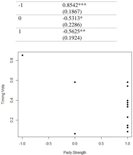
Because the independent variable of party control is partisan-specific, datasets that are built from the restricted dataset is preferred. The dataset cycle+restriction also happened to have the best fit, so those results are shown (Table 11). The results suggest that with a stronger Republican Party, abortion-restriction roll-call votes are scheduled earlier. This implies that a strong party is more motivated to “hide” its controversial roll-call votes from its constituents.
Interestingly, with a strong Democratic Party there appears to be a tendency towards later abortion-restriction roll-call votes. However, because this is a much smaller dataset, this appearance comes from a single data point (Figure 5) which is an issue.
Table 11: Party Control (cycle+restriction) Party Control Coefficient
-1 0.8542*** (0.1867)
0 -0.5313*
(0.2286)
1 -0.5625**
(0.1924)
Figure 5 - Scatterplot, Model 11, Timing Vote vs Party Control (cycle+restricted dataset)
Model 12 uses the party-specific variable of Republican percentage of seats lost/gained per election over the years 2009 – 2016, so my preference is to use datasets derived from the restriction datasets. Of those, the cycle+restriction dataset had the best fit (Table 12). However, the dataset with the best fit overall was the cycle dataset (Table 13), and so both are shown. They both imply that with a greater percentage of Republican seats gained per election, the earlier
roll-call votes are likely to take place. This is similar to the results of Model 11, suggesting that a stronger Republican party prefers to have its controversial votes scheduled earlier in the election cycle where they are less likely to upset constituents. Upon review, it makes sense that the cycle dataset would have stronger results, since it makes sense that a strong party (possibly regardless of affiliation) would want all controversial votes, be they on Republican-sponsored bills or on
Democrat-sponsored bills, to be earlier in the election cycle. Table 12: Seat Loss/Gain (cycle+restriction)
Variable Coefficient (standard error) Seat Loss/Gain -1.20853.
Table 13: Seat Loss/Gain (cycle) Variable Coefficient
(standard error) Seat Loss/Gain -1.31721*
(0.57313)
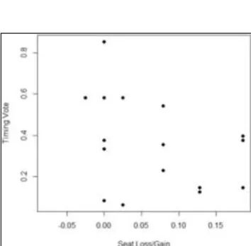
Figure 6 - Scatterplot, Model 12 Timing Vote vs Seat Loss/Gain (cycle dataset)
The results for Model 12 using the complete dataset shown below, for comparison. Contrary to the cycle and cycle+restriction datasets, the professionalism and
professionalism+restriction datasets did not have an improved fit. Table 14: Seat Loss/Gain (complete) Party Control Coefficient
(standard error)
-1 0.7605***
(0.1550)
0 -0.3277.
(0.1713)
1 -0.3822*
(0.1590)
Model 14 also had a party-specific variable: the average vote share per seat the
model (Table 15). The results suggest that a greater average vote share for the Republican Party leads to restriction legislation roll-call votes being scheduled earlier in the election cycle.
Table 15: Avg. Vote Share (cycle+restriction) Variable Coefficient
(standard error) Avg. Vote Share -1.6703**
(0.5279)
Figure 7 - Scatterplot, Model 14, Timing Vote vs Avg Vote Share (cycle+restriction dataset)
The professional and professional+restriction datasets, though a worse fit than cycle+restriction, were still a better fit than the complete and restriction datasets.
After running each independent variable by itself, I ran the categorical and continuous independent variables as multiple linear regressions. Because there are a mix of party-specific and non-party specific variables, I used the restriction only datasets. I got the best fit of the categorical variables when I eliminated cycle_type as a variable and found that cycle+restriction had the best fit (Table 16), though professional+restriction was a better fit than the simple restriction dataset. The relationships and correlations described in the previous analyses remained.
Table 16: Multiple (cycle+restriction) Variable Coefficient
Control Change: 1
0.07292 (0.12268) Party Control: 0 -0.74479**
(0.23758) Party Control: 1 -0.72396**
(0.22117) Professionalism:
0
-0.21354. (0.10625)
For the continuous variables, I found the most useful results came from the cycle dataset, as they were somewhat significant along with having a reasonable R2 value of 0.4819 (Table 17).
Table 17: Multiple (cycle) Variable Coefficient
(standard error) Seat Loss/Gain -1.0287.
(0.4929) Avg. Vote Share -1.4663*
(0.5068)
However, because they are party-specific I am showing the cycle+restriction results as well, though the only result of some significance here is of the average vote share (Table 18). The professional+restriction dataset had less significance and a smaller R2 value of 0.4652, but it was still a better fit than the restriction dataset.
Table 18: Multiple (cycle+restriction) Variable Coefficient
(standard error) Seat Loss/Gain -0.8876
(0.5279) Avg. Vote Share -1.4898*
(0.5130)
Conclusions
conclusions. For Stage 2 in particular I was unsatisfied with the poor fit of the variables, which prevents me from drawing satisfactory conclusions from them. However, what I hoped to accomplish was to establish a baseline from which further study could operate, and there do appear to be three clear trends in Stage 3:
1. Three measures of party strength that I had (party control [over 60% of seats], average percent Republican seats gained per election, and average Republican vote share in a single election: Models 11, 12, and 14, respectively) all indicated that with a strong Republican party, controversial abortion roll-call votes were scheduled earlier in the election cycle, as predicted by Hypothesis 1.
2. The cycle and cycle+restriction datasets were frequently the best fit for the models. Because the “cycle” in question was the 48-month non-staggered cycle, this is in
agreement with Hypothesis 2 which states that longer, non-staggered cycles will have more evident patterns than other cycles.
3. The professional and professional+restriction was not usually the best fit for the models, it was almost always a better fit than the complete dataset. This is in agreement with Hypothesis 3, which states that more professional senates will have more evident patterns than less professional senates.
Going forward, there are several possible ways to improve and clarify the trends shown in this study. First and foremost, increasing the amount of data. Though the original dataset was reasonably large with 229 data points, because of all the variety within those data points, when more datasets were created they became quite small, so even the appearance of a reasonable model fit is in question. Perhaps broadening the definition of abortion legislation, or adding other sorts of controversial legislation with clear party splits (i.e., gun control legislation or LGBTQ+ legislation) could help broaden the data pool.
Secondly, narrowing the focus of the study could be beneficial. Fifty senates allows for a wide variety between senates. This is not a bad thing, but there are potential benefits to, for example, studying senates as geographic groups, or potentially studying separately how the Republican and Democrat parties treat various types of legislation. Doing case studies of key state senates could also be beneficial.
Thirdly, using more precise modeling. I did simple binomial logistic regressions and linear regressions, but taking the time to find the best model possible for each variable could be much more illuminating.
Fourthly, there are a large number of potential confounding variables that I did not cover. These include the makeup and partisanship of the constituents, the varying scheduling rules and practices of individual senates, the partisanship of the Governorship and the House, varying incumbency election laws, and the possible effect of incumbency on voting behaviors and re-election confidence.
Amacher, R.C., Boyes, W.J. (1978). Cycles in senatorial voting behavior: implications for the optimal frequency of elections. Public Choice 33(3), 5.
Brady D., Schwartz E. (1995). Ideology and interests in congressional voting: the politics of abortion in the U.S. Senate. Public Choice 84; 25-48.
Jackson, J.E. (2014). Constituencies and Leaders in Congress: Their Effects on Senate Voting Behavior. Harvard Political Studies. E-book.
Lee, D.S., Moretti, E., Butler, M.J. (2002). Credibility and Policy Convergence: Evidence from US Roll Call Voting Records. Cambridge: National Bureau of Economic Research. Levitt, S.D. (1996). How do senators vote? Disentangling the role of voter preferences, party
affiliation, and senator ideology. The American Economic Review, 86(3), 425.
Mayhew, D. R. (1974). Congress: The electoral connection. New Haven: Yale University Press. Rogers, S. (2017). Electoral Accountability for State Legislative Roll Calls and Ideological
Representation. The American Political Science Review, 111(3), 555-571.