A simulation study on estimating biomarker–treatment interaction effects in randomized trials with prognostic variables

(1)

M E T H O D O L O G Y

Open Access

A simulation study on estimating

biomarker–treatment interaction effects in

randomized trials with prognostic variables

Bernhard Haller

*

and Kurt Ulm

Abstract

Background: To individualize treatment decisions based on patient characteristics, identification of an interaction between a biomarker and treatment is necessary. Often such potential interactions are analysed using data from randomized clinical trials intended for comparison of two treatments. Tests of interactions are often lacking statistical power and we investigated if and how a consideration of further prognostic variables can improve power and decrease the bias of estimated biomarker–treatment interactions in randomized clinical trials with time-to-event outcomes. Methods: A simulation study was performed to assess how prognostic factors affect the estimate of the

biomarker–treatment interaction for a time-to-event outcome, when different approaches, like ignoring other prognostic factors, including all available covariates or using variable selection strategies, are applied. Different scenarios regarding the proportion of censored observations, the correlation structure between the covariate of interest and further potential prognostic variables, and the strength of the interaction were considered.

Results: The simulation study revealed that in a regression model for estimating a biomarker–treatment interaction, the probability of detecting a biomarker–treatment interaction can be increased by including prognostic variables that are associated with the outcome, and that the interaction estimate is biased when relevant prognostic variables are not considered. However, the probability of a false-positive finding increases if too many potential predictors are included or if variable selection is performed inadequately.

Conclusions: We recommend undertaking an adequate literature search before data analysis to derive information about potential prognostic variables and to gain power for detecting true interaction effects and pre-specifying analyses to avoid selective reporting and increased false-positive rates.

Keywords: Biomarker–treatment interaction, Randomized trial, Stratified medicine, Predictive covariates, Variable selection

Background

Treatment individualization, i.e. finding the right treat-ment with the right dose at the right time for a spe-cific patient based on certain patient characteristics, is one of the great goals in modern medicine [1]. One requirement for treatment individualization based on, e.g. a certain biomarker like a genetic characteristic or a blood parameter, is the existence of a relevant associa-tion between the biomarker and the treatment effect [2], often referred to as the biomarker–treatment interaction.

*Correspondence:[email protected]

Institute of Medical Informatics, Statistics and Epidemiology, Technical University of Munich, Ismaninger Str. 22, 81675 Munich, Germany

Only a small number of trials have been planned to analyse biomarker–treatment interactions [3], but often the asso-ciation between one or more biomarkers and a treatment effect is evaluated post hoc in data collected in ran-domized clinical trials intended for overall comparison of treatment groups, like e.g. the detection of the association between the response to cetuximab and the presence or absence of the K-ras mutation in the tumours of patients with advanced colorectal cancer [4].

While often the treatment effect is analysed in dif-ferent subgroups (pre-specified or post hoc specified) to identify patients that benefit from one or another

(2)

treatment [5], it is widely recognized that the compar-ison of treatment groups in many different subgroups can lead to spurious results [6]. Therefore, it is often recommended to assess the biomarker–treatment inter-action in a regression model, which directly allows us to estimate and test for an interaction effect under com-mon model assumptions [7]. Various authors who provide methods for estimating biomarker–treatment interactions stress the importance of the adequate inclusion of prog-nostic factors in the model [8, 9]. For treatment effect estimation in a randomized clinical trial, the European Medicines Agency’s guideline on ‘Points to consider on adjustment for baseline covariates’ recommends including other prognostic factors, i.e. covariates that are assumed to be associated with the outcome, as covariates in the regression model to increase the precision of the esti-mate of the treatment effect [10]. Furthermore, it has been shown that the estimate for the treatment effect is biased in a Cox regression model, if relevant prognos-tic covariates are not included [11]. While defining the model used for effect estimation and hypothesis testing a priori and including all relevant covariates can be con-sidered as best practices [12], adequate information about prognostic factors might not be available for all research questions, especially when molecular information that has not been well studied and for which limited informa-tion from prior investigainforma-tions is available is included in a regression model. Various approaches to determining the covariates that are to be included in a regression model are presented in the literature [13].

The focus of this article is estimating the interaction between one certain pre-specified biomarker of major interest and the treatment. A simulation study was per-formed to evaluate how the presence and inclusion of further prognostic covariates affect the estimate of the biomarker–treatment interaction. Different strategies for model building, such as including only the main effects of treatment, the biomarker and their interaction, addi-tionally including covariates that are significantly associ-ated with the outcome, or using variable selection meth-ods based on Akaike’s information criterion (AIC) [14] are considered. Scenarios with varying proportions of censored observations, different strengths of association of the prognostic covariates and the outcome, differ-ent correlations between prognostic covariates and the biomarker of interest, and different numbers of potential prognostic covariates are considered. The different strate-gies of covariate inclusion are compared in the control of type I error probabilities and the power to reject the null hypothesis of no biomarker–treatment interaction. A special focus was placed on the so-called rule of ten [12,15]. This is often considered for predictive models, but (to the best of our knowledge) has not been investi-gated for the number of additional covariates considered

in a regression model, when the primary goal was estima-tion of an interacestima-tion effect.

Methods

Assessing the biomarker–treatment interaction

The interaction between a continuous biomarker of major interestB, or a continuous covariate in general, and treat-ment T, which is assumed to be binary throughout the article (T ∈ {0; 1}), can be assessed by including an inter-action term between the biomarker and the treatment in an adequate regression model. This means the prod-uct of B andT is included in the regression model as an additional covariate (see e.g. [13]). The Cox regres-sion model [16], also known as the proportional hazards model, is commonly considered in the analysis of survival data in medical research. In the Cox model, the effect of the biomarkerB, the treatmentT, their interactionT×B

andKother covariates described through the matrix Xk

on the hazard rate λ(t)is modelled as

λ(t|T,B,Xk)=λ0(t)exp(βTT+βBB+βT×BT×B+βkTXk),

(1)

where a linear association between a covariate and the log-hazard ratio is assumed. In Eq. (1),λ0(t)is the (unspeci-fied) baseline hazard rate,βTthe regression coefficient for treatmentT,βBthe coefficient for the biomarker of inter-estB,βT×Bthe regression coefficient for their interaction term andβkthe vector of regression coefficients for the Kadditional covariates,X1,. . .,XK. When an interaction term is present, the main effects of the treatmentT and the biomarkerBcan be interpreted as the expected treat-ment difference at a (fictitious) biomarker value ofB= 0 and the effect of the biomarkerBunder treatmentT = 0 conditional on all other covariates. Regression coefficients are estimated by numerical maximization of the partial log-likelihood PL(β). The variance-covariance matrix of the estimated regression coefficients can be derived as the inverse of the observed information matrix I−1(βˆ) (see e.g. [16] or [17] for more details).

Strategies for covariate inclusion

(3)

investigated. The names are used for the models/strategies in the figures and tables presented in this article:

• Main: A model including only the main effects of treatmentT and the biomarker B and their interactionT×B, ignoring all other possible prognostic covariates.

• True: A model including the main effects of treatmentT, the biomarker of interest B and their interactionT×B, as well as all covariates that are truly associated with the outcome, indicating perfect prior knowledge of relevant covariates.

• AICA: A model that includes the main effects of

treatmentT and the biomarker B and their

interactionT×Band additionally all covariates that were selected in a forward variable selection

procedure based on Akaike’s information criterion (AIC) [14] givenT, B andT×Bare included (a model includingT, B andT×Bwas used as a starting and minimal model). Additional covariates were selected as long as the AIC criterion

AIC=2 ll(βˆ)−2p (2)

was increased, wherell(βˆ)is the partial log-likelihood evaluated at the maximum likelihood estimatorβˆand p is the number of estimated regression coefficients. • AICB: A modelling strategy similar to AICAdescribed

above, but prognostic factors were selected based on the AIC criterion considering just the main effect of treatmentT as a starting model and not including B orT×Bin the variable selection process. After prognostic factors were chosen according to the AIC criterion,B andT×Bwere added to the model to estimate the biomarker–treatment interaction. • Significance: A model that includes the main effects

of treatmentT, the covariate of interest and their interaction, as well as all covariates that were significantly associated with the outcome in a Cox regression model including only one covariate (often referred to as univariate Cox models in the medical literature). While this strategy is generally not recommended from a statistical point of view [18], it appears to be a quite popular approach in practice. • Full: A model that includes the treatmentT, the

biomarkerB and their interactionT×Bas

covariates as well as the main effects of allK potential predictorsX1,. . .,XK.

Data generation and simulation settings

Numerous different settings were considered to evalu-ate the modelling strevalu-ategies under varying conditions. For each simulation scenario, 500 subjects were generated. The matrix of continuous covariates (covariate of inter-estBand potential predictorsX1,. . .,XK) was drawn from

a multivariate normal distribution using the R package

mvtnorm[19]. For each variable, a mean of 0 and a stan-dard deviation of 1 were used. The correlation structure was specified as described below. Since a randomized con-trolled trial was intended to be simulated, the treatment variable was drawn independently from all other patient characteristics with Pr(T = 1) = Pr(T = 0) = 0.50 for each individual. For all scenarios,βTandβBwere chosen asβT = ln(0.75) = −0.288 (i.e. exp(βT) = 0.75) and

βB=ln(1.25)=0.223 (i.e. exp(βB)=1.25).

For each scenario, a time-constant baseline hazard rate of λ0(t) = 1 was used. The hazard rate for each indi-vidual was calculated according to Eq.1considering the patient’s characteristics and the regression coefficients for the specific scenario. Event times were generated from an exponential distribution using each individual’s haz-ard rate. All aspects of the simulation study including data generation, estimating regression coefficients and sum-marizing the results were performed with the statistical software R [20].

The following aspects were varied in the simulation study.

Censoring distribution Administrative censoring after 5 years was assumed for all scenarios. Additionally, cen-soring times were generated independently of the event times from an exponential distribution. The hazard rate of the censoring distribution was chosen to produce scenar-ios with

1. a low proportion of censored observations (between 30% and 40% censored observations corresponding to 300 to 350 observed events)

2. a high proportion of censoring (between 60% and 70% censored observations corresponding to 150 to 200 observed events).

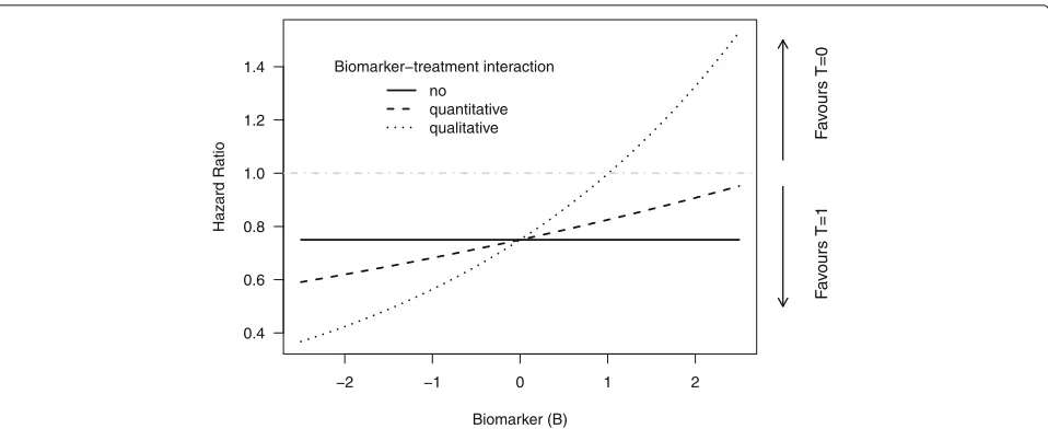
Strength of interaction The strength of the interaction effect between the covariate of interestBand treatmentT

was varied to consider scenarios with no, quantitative or qualitative biomarker–treatment interaction [21] (see also Fig.1):

1. Simulation of data under the null hypothesis of no biomarker–treatment interaction:βT×B=0.

2. Quantitative biomarker–treatment interaction with a difference in the magnitude of the treatment effect between individuals with a low value ofB and individuals with a large value ofB :

βT×B=ln(1.1)=0.095, leading to a hazard ratio

(4)

−2 −1 0 1 2 0.4

0.6 0.8 1.0 1.2 1.4

Biomarker (B)

Hazard Ratio

Biomarker−treatment interaction

no quantitative

qualitative _Fav

ours T=0

F

a

v

ours T=1

Fig. 1Illustration of the different strengths of interaction used in the simulation study. A hazard ratio larger than 1 indicates a higher risk for death under treatmentT₌1, and a hazard ratio below 1 a higher risk under treatmentT₌0. For the scenario with no biomarker–treatment interaction, the hazard ratio between the treatment groups is independent of the biomarker value. For the scenario with a quantitative biomarker–treatment interaction, the risk for an event is smaller underT₌1 compared toT₌0 for all (probable) values ofB, but the difference between groups decreases with increasing values ofB. For the scenario with a qualitative biomarker–treatment interaction, the risk for an event is lower forT₌1 compared toT₌0 for small values ofBand vice versa for large values ofB

3. Qualitative biomarker–treatment interaction indicating an expected lower risk for an event from treatmentT =1for patients with a small value ofB and a lower risk under treatmentT =0for patients with a large value ofB :βT×B=ln(1.33)=0.285,

providing a hazard ratio between the treatment groups smaller than 1 forB<1and a hazard ratio larger than 1 forB>1(dotted line in Fig.1).

Number of potential prognostic variables to be included in the model Three settings for the numberK

of potential candidate predictors that can be included in the regression model were considered:

1. K =12: Here 12 additional prognostic covariates are considered, so the rule of ten is fulfilled under both censoring distributions for most simulation runs, as 150 to 200 events are expected in the settings with a high amount of censoring and up to 15 regression coefficients are to be estimated (12 prognostic variables plus the main effects of treatmentT and the covariate of interestB and their interactionT×B). 2. K =24: Here 24 additional prognostic covariates are

considered, so the rule of ten will be violated for most scenarios with high censoring.

3. K =36: Here 36 additional prognostic covariates are considered. Again, the rule of ten will be violated under high censoring.

Correlation structure between prognostic variables and covariate of interest Three different correlation

structures between the covariate of interest B and the potential prognostic variables X1,. . .,XK were consid-ered:

1. Firstly, a scenario with a biomarker of interestB that is independent of the potential prognostic variables, and independence between all the prognostic variables was investigated, with

1=

⎛ ⎜ ⎜ ⎜ ⎜ ⎜ ⎝

1 0 · · · 0 0 1 0 · · · 0

..

. . .. ...

0 · · · 0 1 0 0 · · · 0 1

⎞ ⎟ ⎟ ⎟ ⎟ ⎟ ⎠

.

2. As a second setting, the correlation coefficients betweenB and all other covariatesX1,. . .,XK, as

well as between each pair of covariatesXi,Xjwith

i=jwas set tor=0.5, indicating a moderate correlation between all variables:

2=

⎛ ⎜ ⎜ ⎜ ⎜ ⎜ ⎝

1 0.5 · · · 0.5 0.5 1 0.5 · · · 0.5

..

. . .. ...

0.5 · · · 0.5 1 0.5 0.5 · · · 0.5 1

⎞ ⎟ ⎟ ⎟ ⎟ ⎟ ⎠

.

[image:4.595.59.538.85.281.2]

(5)

correlation ofr=0.4for another set and a

correlation ofr=0.1orr=0for the other variables:

3= ⎛ ⎜ ⎜ ⎜ ⎜ ⎜ ⎜ ⎜ ⎜ ⎜ ⎜ ⎜ ⎜ ⎜ ⎜ ⎜ ⎜ ⎜ ⎜ ⎜ ⎜ ⎝

1 0.7 0.7 0.7 0.4 0.4 0.4 0.4 0.1 0.1 0.1 0 0 0.7 1 0.7 0.7 0.4 0.4 0.4 0.4 0.1 0.1 0.1 0 0 0.7 0.7 1 0.7 0.4 0.4 0.4 0.4 0.1 0.1 0.1 0 0 0.7 0.7 0.7 1 0.4 0.4 0.4 0.4 0.1 0.1 0.1 0 0 0.4 0.4 0.4 0.4 1 0.4 0.4 0.4 0.1 0.1 0.1 0 0 0.4 0.4 0.4 0.4 0.4 1 0.4 0.4 0.1 0.1 0.1 0 0 0.4 0.4 0.4 0.4 0.4 0.4 1 0.4 0.1 0.1 0.1 0 0 0.4 0.4 0.4 0.4 0.4 0.4 0.4 1 0.1 0.1 0.1 0 0 0.1 0.1 0.1 0.1 0.1 0.1 0.1 0.1 1 0.1 0.1 0 0 0.1 0.1 0.1 0.1 0.1 0.1 0.1 0.1 0.1 1 0.1 0 0 0.1 0.1 0.1 0.1 0.1 0.1 0.1 0.1 0.1 0.1 1 0 0 0.0 0.0 0.0 0.0 0.0 0.0 0.0 0.0 0.0 0.0 0.0 1 0 0.0 0.0 0.0 0.0 0.0 0.0 0.0 0.0 0.0 0.0 0.0 0 1

⎞ ⎟ ⎟ ⎟ ⎟ ⎟ ⎟ ⎟ ⎟ ⎟ ⎟ ⎟ ⎟ ⎟ ⎟ ⎟ ⎟ ⎟ ⎟ ⎟ ⎟ ⎠ .

For the scenarios withK = 24 orK = 36 potential predictors, the correlation matrices were adapted accordingly.

Strength of association between prognostic variables and outcome For the strength of association between the potential prognostic variablesX1,. . .,XKand the out-come, two different settings were chosen:

1. For all covariatesX1,. . .,XK, the same regression

coefficient was chosen:

βk=βeq=(ln(1.1),. . ., ln(1.1))T =(0.095,. . ., 0.095)T.

2. Varying strengths of association between the potential predictors and the risk for an event were considered. The vector of regression coefficients was chosen to be

βk=βv=

⎛ ⎜ ⎜ ⎜ ⎜ ⎜ ⎜ ⎜ ⎜ ⎜ ⎜ ⎜ ⎜ ⎜ ⎜ ⎜ ⎝

ln(1.2) ln(1.1) ln(1) ln(1.2) ln(1.1) ln(1)

.. . ln(1.2) ln(1.1) ln(1)

⎞ ⎟ ⎟ ⎟ ⎟ ⎟ ⎟ ⎟ ⎟ ⎟ ⎟ ⎟ ⎟ ⎟ ⎟ ⎟ ⎠ = ⎛ ⎜ ⎜ ⎜ ⎜ ⎜ ⎜ ⎜ ⎜ ⎜ ⎜ ⎜ ⎜ ⎜ ⎜ ⎜ ⎝ 0.182 0.095 0 0.182 0.095 0 .. . 0.182 0.095 0 ⎞ ⎟ ⎟ ⎟ ⎟ ⎟ ⎟ ⎟ ⎟ ⎟ ⎟ ⎟ ⎟ ⎟ ⎟ ⎟ ⎠ .

As all combinations of the different settings described above were considered in the simulation study, a total of 2 censoring distributions × 3 strengths of interac-tion between biomarkerBand treatmentT ×3 numbers of potential prognostic variables × 3 different correla-tion structures×2 settings for association between the potential prognostics variables and the outcome = 108 settings were considered in the simulation. For each of these settings, 1000 simulation runs were performed.

Analysis and presentation of results

In each simulation run, all of the methods or strategies described in “Strategies for covariate inclusion” section were fitted or applied, respectively. Estimation of the regression coefficients from the Cox regression models was performed with the function coxph in thesurvival

library [22] of the statistical software R [20]. For the vari-able selection based on the AIC criterion, the function

stepAICin the libraryMASS[23] was applied.

For each model in each simulation run, the estimated regression coefficient for the biomarker–treatment inter-action termβˆT×Band its estimated variance as well as the

pvalue of the Wald test for the null hypothesisv H0:βT×B=0 was saved. Additionally, a 95% confidence interval for

βT×Bwas estimated as 95% ci=

ˆ

βT×B−φ0.975 var(βˆT×B);

ˆ

βT×B+φ0.975 var(βˆT×B)

,

(3)

whereφ0.975 denotes the 97.5% quantile of the standard normal distribution andvar(βˆT×B)is the estimated vari-ance of the interaction coefficient obtained in the cor-responding simulation run for the respective modelling approach. If the algorithm for numerical maximization of the partial log-likelihood did not converge, this infor-mation was saved. All results presented in ‘Results’ rely on only estimations for which the numerical optimization algorithm converged. The number of runs for which no result was returned is presented.

For each model and strategy, the confidence interval coverage, i.e. the fraction of simulation runs in which the estimated confidence interval for the biomarker– treatment interaction covered the true value, was derived. The proportion of simulation runs in which the null hypothesis was rejected and a statistically significant biomarker–treatment interaction was detected for the conventional significance level of 5%, i.e. the power of the statistical test if H0were false or the probability of a type I error if H0were true (βT×B=0), was determined [24].

Results

The observed proportions of rejected null hypotheses are summarized in Table 1. Results are presented stratified for different values ofK, strength of interaction and pro-portion of censored observations, but were aggregated over different values of βk and. In Tables 2, 3 and4,

(6)

[image:6.595.61.539.107.386.2]

Table 1Proportions of rejected null hypotheses and numbers of included covariates stratified for number of potential prognostic variables (K), strength of interaction and proportion of censored observations

K Interaction Censoring Main True AICA AICB Significance Full

12 No Low 0.058 0.060 0.062 0.056 0.059 0.060

12 No High 0.054 0.051 0.056 0.048 0.053 0.054

12 Quantitative Low 0.118 0.133 0.139 0.131 0.130 0.134

12 Quantitative High 0.095 0.100 0.108 0.099 0.096 0.099

12 Qualitative Low 0.579 0.663 0.663 0.654 0.653 0.661

12 Qualitative High 0.393 0.437 0.441 0.424 0.432 0.436

24 No Low 0.065 0.058 0.067 0.056 0.057 0.058

24 No High 0.057 0.062 0.073 0.054 0.059 0.063

24 Quantitative Low 0.115 0.135 0.150 0.131 0.131 0.136

24 Quantitative High 0.094 0.100 0.114 0.092 0.100 0.103

24 Qualitative Low 0.465 0.634 0.645 0.616 0.610 0.633

24 Qualitative High 0.349 0.411 0.426 0.383 0.399 0.415

36 No Low 0.065 0.059 0.078 0.056 0.061 0.063

36 No High 0.067 0.068 0.085 0.057 0.066 0.071

36 Quantitative Low 0.114 0.132 0.153 0.118 0.130 0.134

36 Quantitative High 0.093 0.102 0.127 0.093 0.101 0.108

36 Qualitative Low 0.412 0.618 0.629 0.578 0.576 0.610

36 Qualitative High 0.302 0.406 0.431 0.367 0.382 0.402

Results are aggregated over different values ofβkand. For the scenarios with no true biomarker–treatment interaction, results for methods/strategies with an observed

type I error probability above 7% are in italics. For scenarios with a true biomarker–treatment interaction, the observed power is in bold if the type I error probability did not exceed 7%

probability of 7% was considered to be acceptable. For sce-narios with no interaction (βT×B = 0), observed type I

error proportions larger than 7% are in italics. For scenar-ios with data generated underH1(quantitative interaction and qualitative interaction), the proportions of rejected null hypotheses are in bold if the type I error probabil-ity for the approach at the given scenario was not larger than 7%.

The mean numbers of included additional covariates are given for each method or strategy for sets of scenarios stratified forβk and amount of censoring in the bottom

rows of Tables2,3and4and for each of the 108 simulated scenarios in Additional file7: Table S1 (forK=12), Addi-tional file8: Table S2 (forK = 24) and Additional file9: Table S3 (forK=36).

The distributions of the obtained estimates are illus-trated in Fig. 2 for one exemplary set of scenarios. The observed distributions of the regression coeffi-cient estimates for the biomarker–treatment interaction

ˆ

βT×B are displayed as box plots for the scenarios with = 3, βk=βv and low (a) or high number of

cen-sored observations (b). In the top rows, scenarios with no true biomarker–treatment interaction are shown, and in the bottom rows, results for data simulated with true qualitative biomarker–treatment interactions are pre-sented. Scenarios with different numbers of (potential)

prognostic variables (K = 12, K = 24 and K = 36) are shown in separate columns. Distributions of estimated regression coefficients are illustrated for all scenarios with no true interaction (under H0) or with true qualitative interaction in Additional file1: Figure S1, Additional file2: Figure S2, Additional file3: Figure S3, Additional file4: Figure S4, Additional file 5: Figure S5 and Additional file6: Figure S6. In each figure, the true value of the inter-action regression coefficient is illustrated by the horizon-tal red line. Additionally, the confidence interval coverage for each modelling strategy (triangles and blue lines) and the probability of rejection of the null hypothesis of no biomarker–treatment interaction, i.e. the estimated prob-ability for a type I error in the first row and the observed power in the second row, are illustrated (circles and green lines).

(7)

[image:7.595.58.540.97.624.2]

Table 2Proportions of rejected null hypotheses and numbers of included covariates for scenarios withK=12

K _βk Censoring Main True AICA AICB Significance Full

No interaction

12 1 βeq Low 0.066 0.069 0.072 0.066 0.067 0.069

12 1 βv Low 0.051 0.059 0.059 0.055 0.052 0.058

12 2 βeq Low 0.050 0.051 0.054 0.048 0.051 0.051

12 2 βv Low 0.060 0.047 0.052 0.047 0.052 0.052

12 3 βeq Low 0.060 0.065 0.066 0.061 0.063 0.065

12 3 βv Low 0.063 0.066 0.067 0.060 0.067 0.065

12 1 βeq High 0.057 0.056 0.060 0.054 0.055 0.056

12 1 βv High 0.038 0.040 0.037 0.034 0.040 0.044

12 2 βeq High 0.057 0.046 0.054 0.044 0.046 0.046

12 2 βv High 0.060 0.047 0.058 0.049 0.055 0.055

12 3 βeq High 0.053 0.059 0.060 0.050 0.062 0.059

12 3 βv High 0.057 0.056 0.064 0.055 0.061 0.065

Quantitative interaction

12 1 βeq Low 0.122 0.137 0.143 0.121 0.123 0.137

12 1 βv Low 0.119 0.134 0.139 0.132 0.134 0.136

12 2 βeq Low 0.105 0.131 0.136 0.129 0.131 0.131

12 2 βv Low 0.113 0.131 0.141 0.135 0.132 0.132

12 3 βeq Low 0.129 0.146 0.148 0.146 0.141 0.146

12 3 βv Low 0.121 0.121 0.127 0.120 0.116 0.120

12 1 βeq High 0.098 0.109 0.120 0.109 0.100 0.109

12 1 βv High 0.108 0.112 0.118 0.111 0.108 0.111

12 2 βeq High 0.077 0.088 0.099 0.086 0.088 0.088

12 2 βv High 0.104 0.095 0.106 0.096 0.093 0.093

12 3 βeq High 0.086 0.093 0.095 0.091 0.088 0.093

12 3 βv High 0.095 0.101 0.107 0.098 0.100 0.101

Qualitative interaction

12 1 βeq Low 0.625 0.685 0.673 0.662 0.644 0.685

12 1 βv Low 0.605 0.664 0.664 0.661 0.649 0.661

12 2 βeq Low 0.517 0.641 0.641 0.634 0.641 0.641

12 2 βv Low 0.521 0.646 0.648 0.643 0.644 0.644

12 3 βeq Low 0.621 0.678 0.686 0.673 0.680 0.678

12 3 βv Low 0.583 0.661 0.664 0.652 0.661 0.658

12 1 βeq High 0.427 0.462 0.464 0.446 0.433 0.462

12 1 βv High 0.424 0.438 0.447 0.432 0.440 0.443

12 2 βeq High 0.338 0.403 0.410 0.389 0.403 0.403

12 2 βv High 0.359 0.431 0.429 0.413 0.433 0.433

12 3 βeq High 0.394 0.424 0.425 0.407 0.420 0.424

12 3 βv High 0.418 0.466 0.471 0.456 0.465 0.449

Mean number of prognostic covariates included

βeq Low 0 12 6.8 7.3 8.7 12

βv Low 0 8 6.4 6.9 8.7 12

βeq High 0 12 5.1 5.7 8.0 12

βv High 0 8 5.3 5.8 8.2 12

For the scenarios with no true biomarker–treatment interaction, results for methods/strategies with an observed type I error probability above 7% are in italics. For scenarios with a true biomarker–treatment interaction, the observed power is in bold if the type I error probability did not exceed 7%

increased type I error probabilities were observed for each method for at least one scenario, except for AICB. For AICA, type I error probabilities above 7% were observed for six of the 12 settings (Table3) and for scenarios with a high proportion of censored observations (60% to 70%) when scenarios with differentβkandwere aggregated

(8)

[image:8.595.57.539.100.625.2]

No interaction

24 1 βeq Low 0.044 0.049 0.065 0.053 0.048 0.049

24 1 βv Low 0.055 0.069 0.074 0.065 0.060 0.069

24 2 βeq Low 0.087 0.052 0.063 0.046 0.052 0.052

24 2 βv Low 0.068 0.071 0.081 0.066 0.071 0.071

24 3 βeq Low 0.068 0.049 0.061 0.052 0.055 0.049

24 3 βv Low 0.066 0.056 0.061 0.053 0.054 0.056

24 1 βeq High 0.035 0.056 0.069 0.054 0.046 0.056

24 1 βv High 0.051 0.071 0.076 0.059 0.068 0.076

24 2 βeq High 0.073 0.066 0.074 0.056 0.066 0.066

24 2 βv High 0.060 0.054 0.066 0.048 0.056 0.056

24 3 βeq High 0.062 0.058 0.073 0.047 0.059 0.058

24 3 βv High 0.059 0.068 0.079 0.060 0.057 0.066

24 1 βeq Low 0.114 0.142 0.158 0.137 0.122 0.142

24 1 βv Low 0.106 0.138 0.150 0.132 0.125 0.143

24 2 βeq Low 0.119 0.135 0.148 0.130 0.135 0.135

24 2 βv Low 0.111 0.124 0.145 0.117 0.126 0.126

24 3 βeq Low 0.121 0.136 0.145 0.128 0.141 0.136

24 3 βv Low 0.121 0.136 0.157 0.141 0.134 0.136

24 1 βeq High 0.088 0.100 0.117 0.091 0.093 0.100

24 1 βv High 0.085 0.104 0.110 0.096 0.094 0.111

24 2 βeq High 0.094 0.109 0.122 0.094 0.109 0.109

24 2 βv High 0.113 0.096 0.116 0.088 0.100 0.100

24 3 βeq High 0.082 0.098 0.109 0.097 0.103 0.098

24 3 βv High 0.100 0.091 0.109 0.086 0.098 0.098

24 1 βeq Low 0.630 0.697 0.686 0.658 0.632 0.697

24 1 βv Low 0.547 0.678 0.688 0.656 0.615 0.685

24 2 βeq Low 0.349 0.610 0.619 0.595 0.610 0.610

24 2 βv Low 0.358 0.590 0.608 0.584 0.578 0.578

24 3 βeq Low 0.443 0.596 0.620 0.582 0.587 0.596

24 3 βv Low 0.465 0.632 0.651 0.621 0.636 0.631

24 1 βeq High 0.448 0.457 0.463 0.424 0.412 0.457

24 1 βv High 0.384 0.453 0.466 0.425 0.420 0.464

24 2 βeq High 0.276 0.364 0.387 0.340 0.364 0.364

24 2 βv High 0.292 0.397 0.423 0.378 0.411 0.411

24 3 βeq High 0.355 0.387 0.405 0.356 0.382 0.387

24 3 βv High 0.338 0.408 0.409 0.377 0.404 0.408

βeq Low 0 24 13.2 13.7 17.5 24

βv Low 0 16 12.7 13.1 17.8 24

βeq High 0 24 10.2 10.7 16.5 24

βv High 0 16 10.6 11.0 16.8 24

proportion of censored observations led to rejection of the null hypothesis in more than 7% of the observed simula-tion runs (2, βeq and1,βeq). For all other scenarios,

the observed type I error probabilities were between 5% and 7%. For the strategy AICB, all observed type I error probabilities were between 5% and 7%.

(9)

[image:9.595.58.540.99.627.2]

No interaction

36 1 βeq Low 0.047 0.065 0.080 0.054 0.056 0.065

36 1 βv Low 0.059 0.067 0.084 0.066 0.069 0.073

36 2 βeq Low 0.077 0.053 0.073 0.051 0.053 0.053

36 2 βv Low 0.075 0.054 0.074 0.052 0.056 0.056

36 3 βeq Low 0.067 0.060 0.083 0.057 0.064 0.060

36 3 βv Low 0.063 0.055 0.074 0.053 0.069 0.069

36 1 βeq High 0.052 0.071 0.086 0.059 0.055 0.071

36 1 βv High 0.047 0.063 0.080 0.058 0.050 0.066

36 2 βeq High 0.085 0.080 0.082 0.057 0.080 0.080

36 2 βv High 0.085 0.064 0.086 0.054 0.070 0.070

36 3 βeq High 0.057 0.069 0.094 0.056 0.063 0.069

36 3 βv High 0.075 0.063 0.081 0.057 0.076 0.071

36 1 βeq Low 0.103 0.150 0.165 0.130 0.138 0.150

36 1 βv Low 0.095 0.131 0.150 0.120 0.125 0.136

36 2 βeq Low 0.121 0.120 0.141 0.109 0.120 0.120

36 2 βv Low 0.128 0.128 0.147 0.121 0.134 0.134

36 3 βeq Low 0.115 0.121 0.142 0.103 0.122 0.121

36 3 βv Low 0.119 0.143 0.172 0.125 0.140 0.143

36 1 βeq High 0.081 0.108 0.133 0.098 0.094 0.108

36 1 βv High 0.095 0.112 0.132 0.101 0.102 0.118

36 2 βeq High 0.100 0.085 0.103 0.072 0.085 0.085

36 2 βv High 0.092 0.109 0.127 0.093 0.118 0.118

36 3 βeq High 0.091 0.104 0.134 0.099 0.105 0.104

36 3 βv High 0.097 0.093 0.132 0.093 0.102 0.115

36 1 βeq Low 0.551 0.652 0.657 0.603 0.558 0.652

36 1 βv Low 0.517 0.700 0.688 0.658 0.599 0.669

36 2 βeq Low 0.280 0.570 0.582 0.518 0.570 0.570

36 2 βv Low 0.266 0.555 0.575 0.517 0.542 0.542

36 3 βeq Low 0.408 0.609 0.637 0.582 0.581 0.609

36 3 βv Low 0.451 0.623 0.637 0.592 0.605 0.620

36 1 βeq High 0.389 0.447 0.456 0.403 0.385 0.447

36 1 βv High 0.390 0.472 0.486 0.437 0.418 0.453

36 2 βeq High 0.219 0.368 0.411 0.334 0.368 0.368

36 2 βv High 0.228 0.385 0.419 0.353 0.389 0.389

36 3 βeq High 0.282 0.364 0.396 0.328 0.352 0.364

36 3 βv High 0.303 0.402 0.416 0.350 0.382 0.391

βeq Low 0 36 19.6 19.9 24.5 36

βv Low 0 24 19.0 19.4 25.2 36

βeq High 0 36 15.2 15.7 23.1 36

βv High 0 24 16.0 16.4 23.9 36

Figure S2B, Additional file3: Figure S3A and Figure S3B, Additional file4: Figure S4A and Figure S4B, Additional file5: Figure S5A and Figure S5B, and Additional file6: Figure S6A and Figure S6B). This also led to a loss of power, which was reduced as compared to the true model for most of the scenarios (Tables 1, 2, 3 and 4,

(10)

a

b

Fig. 2Distribution ofβˆT×Bfor scenarios with=3,βk=βv, and low censoring (a) or high censoring (b) for no biomarker–treatment interaction (βT×B=ln(1.0)=0, top rows) or qualitative biomarker–treatment interaction (βT×B=ln(1.33)=0.285, bottom rows). Scenarios for different numbers of potential prognostic variables are shown in different columns. The dashed red lines indicate the true value ofβT×B, the blue triangles represent the observed confidence interval coverages and the green dots the observed probability for a type I error (a) or estimated power (b). AIC Akaike’s information criterion, qual. qualitative, Sig significance

due to its increased type I error probabilities. The full model is identical to the true model for βk = βeq,

as all covariates are truly associated with the outcome. For βk = βv, the power of the full model was

simi-lar to the power of the true model for K = 12 and

K = 24 in our simulation runs, but was slightly lower for simulations withK = 36. The strategy AICB, which appears to have an adequate false positive rate, showed (slightly) lower power than the true model for (almost) all of the scenarios. A slightly decreased power was also

observed for the strategy including all covariates that were significantly associated with the outcome (significance). The type I error probability was acceptable for most sce-narios with a small or moderate number of potential predictors (K = 12 andK = 24), but an increased type I error probability was observed for scenarios with many potential predictors (K=36).

[image:10.595.63.536.86.534.2]

(11)

was under 93% for 52 of the 108 scenarios (48.1%), indicat-ing standard errors for the regression coefficient of inter-est were underinter-estimated following the variable selection procedure.

In the last rows of Tables2,3 and4, the mean num-bers of additionally included covariates are summarized for each method/strategy stratified for the amount of censoring andβk(which determines the number of truly

prognostic variables). It was observed that for our set-tings, the procedure including variables that were sig-nificantly associated with the outcome in univariate Cox models selected more variables than the AIC-based meth-ods, and that slightly more variables were chosen with AICB than with AICA. For scenarios with βk = βeq,

the true and full models were identical by definition. More detailed information on the numbers of covari-ates included are given in Additional file 7: Table S1, Additional file8: Table S2 and Additional file9: Table S3.

The optimization algorithm for numerical maximiza-tion of the partial log-likelihood of the Cox regression model for estimating the regression coefficients did not converge for some simulation runs. The problem espe-cially occurred for AICA. Over all 108,000 simulation runs (108 scenarios × 1,000 runs per scenario), the estima-tion algorithm did not converge 11 times (0.010%) for main, twice (0.002%) for true, 895 times (0.829%) for AICA, 27 times (0.025%) for AICB, three times (0.003%) for significance and no times (0%) for full.

Discussion

The ultimate goal in individualized or tailored medicine is to find the best treatment for each individual based on the patient’s characteristics like age, sex, co-morbidities, disease history and molecular and genetic information, which are often referred to as biomarkers. The exis-tence and detection of a biomarker–treatment interaction can be considered as a requirement for such treatment individualization [2], and consequently an interaction between the biomarker of interest and treatment has to be established in a first step, e.g. by finding statistically significant and clinically relevant interactions based on data from (multiple) randomized clinical trials. Decision rules for treatment selection based on the characteristics of a certain patient have to be investigated and estab-lished afterwards, also considering the benefits and costs of the application of a certain treatment strategy for a given patient.

To detect relevant associations and interactions, it is well known that splitting a quantitative variable into dif-ferent categories, leading to a comparison of treatment effects between different subgroups, will result in a loss of information and will consequently decrease the prob-ability of detecting a true biomarker–treatment interac-tion [25]. So, using all the quantitative information is

recommended for analysis of biomarker–treatment inter-actions [7]. To estimate a treatment effect in a randomized clinical trial, the inclusion of relevant prognostic vari-ables is recommended [10] to increase the precision of the estimate and consequently the probability of detect-ing real group differences. For this article, we performed a simulation study to investigate whether the probabil-ity of detecting a biomarker–treatment interaction in data derived from a randomized clinical trial can be improved by including further potentially prognostic variables in a Cox regression model for time-to-event data. Differ-ent settings for the strength of interaction between the biomarker and the treatment, the correlation between the biomarker of interest and other potential predictors, the strength of association between the predictors and outcome, the number of (potential) further predictors, and the number of events and censored observations were considered. When a biomarker–treatment interac-tion is assessed using data from a randomized clinical trial, obviously the best choice is to include in the final model all covariates truly associated with the outcome, which was covered by the true model in our simulation study. As this true model often is not known in prac-tice, especially in investigations including molecular or genetic information, more flexible approaches might be needed. So, we also investigated strategies using data-driven variable selection procedures based on AIC [14] or on the results of Cox regression models with single covariates.

(12)

interval coverage. This was not observed in a strategy that selected the relevant prognostic variables in a first step and added the biomarker main effect and the biomarker– treatment interaction afterwards (called AICBin our arti-cle). In our simulated scenarios, the strategy including all covariates that were found to be significantly associated with the outcome performed similarly to that approach. Automated variable selection procedures are criticized in the literature for various reasons (see e.g. [28]). Based on the results of our simulation study, we strongly discour-age using an automated variable selection procedure to choose additional prognostic variables after including the biomarker–treatment interaction of interest, as this may lead to unreliable results.

An obvious limitation of our study is that we observed only a moderate number of different scenarios with three correlation structures, three strengths of inter-action between the biomarker and treatment, two strengths/structures of association between the additional prognostic variables and treatment, two censoring distri-butions, three numbers of (potential) prognostic variables, and a fixed number of 500 observations, due to limited time and space. All these aspects influenced the results and other settings may have led to different findings and consequently recommendations. In particular, the num-ber of observed events, which is more important than the total sample size for a time-to-event outcome, was varied only by choosing two different censoring propor-tions, but it has a major impact on the power of the interaction test. We also investigated only a small number of strategies for inclusion or selection of further covari-ates based on the AIC and significant associations with the outcome. Other strategies (like backward selection), other criteria (like the Bayesian information criterion [29]) or other procedures for variable selection (like the least absolute shrinkage and selection operator [30]) were not considered. Furthermore, we considered only normally distributed biomarkers and linear associations and inter-actions in our simulations and fitted Cox regression mod-els assuming linear associations and time-constant effects to our data. Recently introduced methods for estimat-ing non-linear interactions, like local partial likelihood estimation [31], multivariable fractional polynomials for interaction [8] or the modified covariate approach [9], were not investigated.

It has to be considered that in our scenario, only one pre-specified biomarker of interest is assessed. It was identified as being of interest e.g. in an observational study or was found to be relevant for a similar kind of disease. If more than one biomarker is investigated, multiplicity issues arise that have to be adequately con-sidered [32]. When an analysis is an additional analysis to a standard group comparison for a randomized clini-cal trial, it can only be exploratory in nature. Nevertheless,

the method used for statistical analysis should be specified a priori to generate reliable results and avoid problems of data-dredging and selective reporting, and consequently generating unreliable results and increased false-positive rates [33]. Further algorithms or strategies should be used in sensitivity analyses to assess the stability of the observed results. If the investigation of a biomarker– treatment interaction is of major importance for a clinical trial, this should be considered in the design stage and consequently in the sample size calculation.

Conclusions

Based on the results of our simulation study, we rec-ommend considering prognostic covariates in regression models when estimating biomarker–treatment interac-tions, as the power for detecting true interactions can be increased. However, including too many variables can lead to unreliable results. The choice of variables included should be based on prior information and subject knowl-edge. Automatic variable selection procedures have to be handled with care.

Additional files

Additional file 1: Figure S1. Distribution ofβˆT×Bfor scenarios with

K=12,βk=βeq, and low censoring (A) or high censoring (B) for no biomarker–treatment interaction (βT×B=ln(1.0)=0, top rows) or qualitative biomarker–treatment interaction (βT×B=ln(1.33)=0.285, bottom rows). Results for different correlation structures are shown in separate columns. The dashed red lines indicate the true value ofβT×B, the blue triangles represent the observed confidence interval coverages, the green dots the observed probability for a type I error (A) or estimated power (B). (PDF 20 kb)

K=12,βk=βv, and low censoring (A) or high censoring (B) for no biomarker–treatment interaction (βT×B=ln(1.0)=0, top rows) or qualitative biomarker–treatment interaction (βT×B=ln(1.33)=0.285, bottom rows). Results for different correlation structures are shown in separate columns. The dashed red lines indicate the true value ofβT×B, the blue triangles represent the observed confidence interval coverages, the green dots the observed probability for a type I error (A) or estimated power (B). (PDF 20 kb)

K=24,βk=βeq, and low censoring (A) or high censoring (B) for no biomarker–treatment interaction (βT×B=ln(1.0)=0, top rows) or qualitative biomarker–treatment interaction (βT×B=ln(1.33)=0.285, bottom rows). Results for different correlation structures are shown in separate columns. The dashed red lines indicate the true value ofβT×B, the blue triangles represent the observed confidence interval coverages, the green dots the observed probability for a type I error (A) or estimated power (B). (PDF 20 kb)

(13)

Additional file 5:Figure S5. Distribution ofβˆT×Bfor scenarios with K=36,βk=βeq, and low censoring (A) or high censoring (B) for no biomarker–treatment interaction (βT×B=ln(1.0)=0, top rows) or qualitative biomarker–treatment interaction (βT×B=ln(1.33)=0.285, bottom rows). Results for different correlation structures are shown in separate columns. The dashed red lines indicate the true value ofβT×B, the blue triangles represent the observed confidence interval coverages, the green dots the observed probability for a type I error (A) or estimated power (B). (PDF 20 kb)

Additional file 6:Figure S6. Distribution ofβˆT×Bfor scenarios with

K=36,βk=βv, and low censoring (A) or high censoring (B) for no biomarker–treatment interaction (βT×B=ln(1.0)=0, top rows) or qualitative biomarker–treatment interaction (βT×B=ln(1.33)=0.285, bottom rows). Results for different correlation structures are shown in separate columns. The dashed red lines indicate the true value ofβT×B, the blue triangles represent the observed confidence interval coverages, the green dots the observed probability for a type I error (A) or estimated power (B). (PDF 20 kb)

Additional file 7:Table S1. Mean number of additionally included

prognostic variables for all scenarios withK=12. (PDF 68 kb)

prognostic variables for all scenarios withK=24. (PDF 68 kb)

prognostic variables for all scenarios withK=36. (PDF 68 kb) Acknowledgments

Not applicable

Funding

This work was supported by the German Research Foundation (DFG) and the Technische Universität München within the funding programme Open Access Publishing.

Availability of data and materials

No patient data were used when writing this article. The R code for generating the data sets used in the simulation study, for applying the approaches and strategies described, and for analysing the results obtained in the simulation study can be obtained from the first author upon reasonable request.

Authors’ contributions

BH designed and implemented the simulation study and drafted the manuscript. KU critically reviewed the manuscript for intellectual content. Both authors read and approved the final manuscript.

Ethics approval and consent to participate Not applicable

Consent for publication Not applicable

Competing interests

The authors declare that they have no competing interests.

Publisher’s Note

Springer Nature remains neutral with regard to jurisdictional claims in published maps and institutional affiliations.

Received: 2 November 2017 Accepted: 22 January 2018

References

1. Hamburg MA, Collins FS. The path to personalized medicine. N Engl J Med. 2010;363(4):301–4.

2. Chen JJ, Lu TP, Chen YC, Lin WJ. Predictive biomarkers for treatment selection: statistical considerations. Biomark Med. 2015;9(11):1121–35. 3. Rothwell PM. Subgroup analysis in randomised controlled trials:

importance, indications, and interpretation. Lancet. 2005;365(9454): 176–86.

4. Karapetis CS, Khambata-Ford S, Jonker DJ, O’Callaghan CJ, Tu D, Tebbutt NC, et al. K-ras mutations and benefit from cetuximab in advanced colorectal cancer. N Engl J Med. 2008;359(17):1757–65. 5. Assmann SF, Pocock SJ, Enos LE, Kasten LE. Subgroup analysis and other

(mis)uses of baseline data in clinical trials. Lancet. 2000;355(9209):1064–9. 6. Naggara O, Raymond J, Guilbert F, Roy D, Weill A, Altman DG. Analysis

by categorizing or dichotomizing continuous variables is inadvisable: an example from the natural history of unruptured aneurysms. Am J Neuroradiol. 2011;32(3):437–40.

7. Royston P, Sauerbrei W. Interactions between treatment and continuous covariates: a step toward individualizing therapy. J Clin Oncol. 2008;26(9): 1397–9.

8. Royston P, Sauerbrei W. A new approach to modelling interactions between treatment and continuous covariates in clinical trials by using fractional polynomials. Stat Med. 2004;23(16):2509–25.

9. Tian L, Alizadeh AA, Gentles AJ, Tibshirani R. A simple method for estimating interactions between a treatment and a large number of covariates. J Am Stat Assoc. 2014;109(508):1517–32.

10. Committee for Proprietary Medicinal Products. Points to consider on adjustment for baseline covariates. Stat Med. 2004;23(5):701. 11. Langner I, Bender R, Lenz-Tönjes R, Küchenhoff H, Blettner M. Bias of

maximum-likelihood estimates in logistic and Cox regression models: a comparative simulation study. Sonderforschungsbereich 386. Ludwig-Maximilians-Universität München; 2003.

12. Harrell F. Regression modeling strategies: with applications to linear models, logistic and ordinal regression, and survival analysis. New York: Springer; 2001.

13. Royston P, Sauerbrei W. Multivariable model-building: a pragmatic approach to regression analysis based on fractional polynomials for modelling continuous variables, Vol. 777. Chichester: Wiley; 2008. 14. Akaike H. A new look at the statistical model identification. IEEE Trans

Autom Control. 1974;19(6):716–23.

15. Babyak MA. What you see may not be what you get: a brief, nontechnical introduction to overfitting in regression-type models. Psychosom Med. 2004;66(3):411–21.

16. Cox DR. Regression models and life tables (with discussion). J Royal Stat Soc. 1972;34:187–220.

17. Therneau TM, Grambsch PM. Modeling survival data: extending the Cox model. New York: Springer; 2013.

18. Vach W. Regression models as a tool in medical research. Boca Raton: CRC Press; 2012.

19. Genz A, Bretz F, Miwa X, Tetsuhisa abd Mi, Leisch F, Scheipl F, Hothorn T. Mvtnorm: multivariate normal and T distributions. R package version 1.0-5. 2016.http://CRAN.R-project.org/package=mvtnorm.

20. R Core Team. R: a language and environment for statistical computing. Vienna: R Foundation for Statistical Computing; 2016.https://www.R-project.org/. 21. Polley M-YC, Freidlin B, Korn EL, Conley BA, Abrams JS, McShane LM.

Statistical and practical considerations for clinical evaluation of predictive biomarkers. J Natl Cancer Inst. 2013;105(22):1677–83.

22. Therneau T. A package for survival analysis in S. Version 2.38. 2015.http:// CRAN.R-project.org/package=survival.

23. Venables WN, Ripley BD. Modern applied statistics with S, 4th ed. New York: Springer; 2002.http://www.stats.ox.ac.uk/pub/MASS4. 24. Burton A, Altman DG, Royston P, Holder RL. The design of simulation

studies in medical statistics. Stat Med. 2006;25(24):4279–92. 25. Royston P, Altman DG, Sauerbrei W. Dichotomizing continuous

predictors in multiple regression: a bad idea. Stat Med. 2006;25(1):127–41. 26. Concato J, Peduzzi P, Holford TR, Feinstein AR. Importance of events per

independent variable in proportional hazards analysis. I. Background, goals, and general strategy. J Clin Epidemiol. 1995;48(12):1495–501. 27. Peduzzi P, Concato J, Feinstein AR, Holford TR. Importance of events per

independent variable in proportional hazards regression analysis. II. Accuracy and precision of regression estimates. J Clin Epidemiol. 1995;48(12):1503–10.

28. Sainani KL. Multivariate regression: the pitfalls of automated variable selection. PM&R. 2013;5(9):791–4.

29. Schwarz G, et al. Estimating the dimension of a model. Annals Stat. 1978;6(2):461–4.

(14)

31. Liu Y, Jiang W, Chen BE. Testing for treatment-biomarker interaction based on local partial-likelihood. Stat Med. 2015;34(27):3516–30. 32. European Medicines Agency. Guideline on multiplicity issues in clinical

trials. 2017.http://www.ema.europa.eu/ema/index.jsp?curl=pages/ regulation/general/general_content_001220.jsp&mid=.

33. Ioannidis JP. Why most published research findings are false. PLoS Med. 2005;2(8):124.

• We accept pre-submission inquiries

• Our selector tool helps you to find the most relevant journal

• We provide round the clock customer support

• Convenient online submission

• Thorough peer review

• Inclusion in PubMed and all major indexing services

• Maximum visibility for your research

Submit your manuscript at www.biomedcentral.com/submit