R E S E A R C H A R T I C L E
Practical recommendations for reporting Fine
‐
Gray model
analyses for competing risk data
Peter C. Austin
1,2,3| Jason P. Fine
4,51Institute for Clinical Evaluative Sciences,
Toronto, Ontario, Canada
2Institute of Health Policy, Management
and Evaluation, University of Toronto, Toronto, Ontario, Canada
3Schulich Heart Research Program,
Sunnybrook Research Institute, Toronto, Ontario, Canada
4Department of Biostatistics, University of
North Carolina, Chapel Hill, North Carolina, USA
5Department of Statistics and Operations
Research, University of North Carolina, Chapel Hill, North Carolina, USA
Correspondence
Peter Austin, Institute for Clinical Evaluative Sciences, G106, 2075 Bayview Avenue, Toronto, Ontario M4N 3M5, Canada.
Email: [email protected]
Funding information
Heart and Stroke Foundation; Canadian Institutes of Health Research, Grant/ Award Number: CRT43823, CTP 79847 and MOP 86508; Ontario Ministry of Health and Long‐Term Care (MOHLTC)
In survival analysis, a competing risk is an event whose occurrence precludes the occurrence of the primary event of interest. Outcomes in medical research are frequently subject to competing risks. In survival analysis, there are 2 key questions that can be addressed using competing risk regression models: first, which covariates affect the rate at which events occur, and second, which covariates affect the probability of an event occurring over time. The cause‐ specific hazard model estimates the effect of covariates on the rate at which events occur in subjects who are currently event‐free. Subdistribution hazard ratios obtained from the Fine‐Gray model describe the relative effect of covar-iates on the subdistribution hazard function. Hence, the covarcovar-iates in this model can also be interpreted as having an effect on the cumulative incidence function or on the probability of events occurring over time. We conducted a review of the use and interpretation of the Fine‐Gray subdistribution hazard model in articles published in the medical literature in 2015. We found that many authors provided an unclear or incorrect interpretation of the regres-sion coefficients associated with this model. An incorrect and inconsistent interpretation of regression coefficients may lead to confusion when compar-ing results across different studies. Furthermore, an incorrect interpretation of estimated regression coefficients can result in an incorrect understanding about the magnitude of the association between exposure and the incidence of the outcome. The objective of this article is to clarify how these regression coefficients should be reported and to propose suggestions for interpreting these coefficients.
K E Y W O R D S
competing risks, cumulative incidence function, subdistribution hazard model, survival analysis
1
|
I N T R O D U C T I O N
Survival analysis is concerned with outcomes that occur over time. Two key concepts in survival analysis are the survival function and the hazard function. The survival function, denoted byS(t), is the probability that an individual survives to
-This is an open access article under the terms of the Creative Commons Attribution‐NonCommercial‐NoDerivs License, which permits use and distribution in any medium, provided the original work is properly cited, the use is non‐commercial and no modifications or adaptations are made.
© 2017 The Authors.Statistics in Medicinepublished by John Wiley & Sons Ltd. DOI: 10.1002/sim.7501
timet(ie, the probability that an event occurs after timet). The hazard function, denoted byh(t), is the instantaneous rate of the occurrence of the event of interest in subjects who are currently at risk of the event (or for whom the event has not yet occurred). The Kaplan‐Meier method can be used to obtain an estimate of the survival function,1while the Cox proportional hazards regression model is used to estimate the relative effect of covariates on the hazard function.2 While the regression coefficients from the Cox model describe the relative effect of the covariates on the hazard of the occurrence of the outcome, the following relationship holds:
S tðjXÞ ¼S0ð Þt expð ÞXβ; (1)
whereS(t|X) denotes the survival function for an individual whose set of covariates is equal to X,S0(t) denotes the
base-line survival function (the survival function for a subject whose covariates are all equal to zero), andβdenotes the vector of regression coefficients from the Cox model. Thus, there is a direct correspondence between the effect of a covariate on the hazard of the outcome and the effect of a covariate on the incidence of the outcome: If a covariate increases the haz-ard of the occurrence of the outcome, it also will increase the incidence of the outcome (although the magnitude of the 2 effects can be expected to differ). Thus, making inferences about the direction of the effect of a covariate on the hazard function permits one to make equivalent inferences about the direction of the effect of that covariate on the incidence (or on the probability of the occurrence) of the outcome. This direct correspondence between the effect of a covariate on the hazard function and the effect of the covariate on incidence has allowed authors to be imprecise in their language when interpreting the fitted Cox regression model. Authors have been able to conclude that a given risk factor or covariate increasedthe riskof an event, without specifying whetherriskdenotesthe hazardof an event (ie, the rate of the occur-rence of the event in those still at risk of the event) orthe incidenceof the event (ie, the probability of the occurrence of the event). Strictly speaking, we would argue that risk refers to probabilities and that one should describe the effect of covariates on the rate at which events occur.
We provide a brief example to which we will return throughout this commentary. The data consist of 16 237 patients hospitalized with heart failure between 1999 and 2005 in the Canadian province of Ontario. The data were collected as part of the EFFECT study.3These data are described in greater detail in a recent tutorial on methods for the analysis of survival data in the presence of competing risks.4Subjects were followed for 5 years from the time of hospitalization, and the timing of the occurrence of death (and cause of death) was recorded for each subject. Subjects were censored after 5 years if they had not yet died. Ten thousand two hundred fifteen subjects (62.9%) died within 5 years of hospitalization. Using a Cox proportional hazards model, we regressed the hazard of all‐cause death on patient age and sex. The esti-mated hazard ratios and associated 95% confidence intervals were 1.54 (1.51‐1.57) for a 10‐year increase in age and 1.18 (1.14‐1.23) for males compared to females. Thus, a 10‐year increase in age was associated with a 54% increase in the rate of all‐cause death. Similarly, the rate of death was 18% higher for males than it was for females. Since the hazard ratio for age is greater than 1, one can also conclude that a 10‐year increase in age is associated with an increase in the incidence of all‐cause death, although one cannot formally quantify the magnitude of this association. Similarly, the inci-dence of death is higher in males than in females.
In survival analysis, a competing risk is an event whose occurrence precludes the occurrence of the primary event of interest. If the primary outcome of interest is time to death due to cardiovascular causes, then death due to noncardiovascular causes is a competing risk (eg, subjects who die of cancer are no longer at risk of death due to cardio-vascular causes).4-6In the presence of competing risks, 2 different hazard functions have been defined: the cause‐specific hazard function (formula 2) and the subdistribution hazard function (formula 3).4-6
λcs
kð Þ ¼t Δlimt→0
Probðt≤T<tþΔt;D¼kjT≥tÞ
Δt ; (2)
λsd
kð Þ ¼t Δlimt→0
Probðt≤T<tþΔt;D¼kjT≥t∪ðT<t∩K≠kÞÞ
Δt : (3)
The cause‐specific hazard model estimates the effect of covariates on the cause‐specific hazard function, while the Fine‐ Gray subdistribution hazard model estimates the effect of covariates on the subdistribution hazard function.
The cumulative incidence function (CIF) describes the incidence of the occurrence of an event while taking compet-ing risks into account. The subdistribution hazard model has also been described as a CIF regression model. This latter name makes explicit the link between the subdistribution hazard function and the CIF. Thus, the subdistribution hazard model allows one to estimate the effect of covariates on the CIF for the event of interest. In particular, it permits one to recover a relationship similar in form to that described in formula 1:
1−CIFð Þ ¼t ð1−CIF0ð Þt Þexpð ÞXβ; (4)
(where CIF0denotes the baseline CIF). Thus, if a covariate is associated with an increase in the subdistribution hazard
function, it will also be associated with an increase in the incidence of the event. A survey of the medical literature reported in this paper suggests that in the presence of competing risks, clinical researchers may misinterpret hazard ratios from the Fine‐Gray subdistribution hazard model, similar to what often occurs when interpreting the proportional hazards model in the absence of competing risks. This survey further suggests that such issues may arise in part because of the lack of a clear understanding of the relationships of the subdistribution hazard and the cause specific hazard to the CIF: There is a one‐to‐one relationship with the CIF for the subdistribution hazard but not for the cause‐specific hazard. There are 2 objectives to this commentary. First, to provide guidance on the interpretation of regression coefficients associated with the Fine‐Gray subdistribution hazard model. Second, to review papers published in 2015 in the medical literature that reported using the Fine‐Gray subdistribution hazard model and examine how authors interpreted the regression coefficients associated with the fitted model.
2
|
I N T E R P R E T I N G R E G R E S S I O N C O E F F I C I E N T S F R O M C O M P E T I N G R I S K
R E G R E S S I O N M O D E L S
2.1
|
Cause
‐
specific hazard model regression coefficients
The exponentiated regression coefficient from a cause‐specific hazard model denotes the magnitude of the relative change in the cause‐specific hazard function associated with a 1‐unit change in the covariate. Therefore, the cause‐ spe-cific hazard ratio denotes the relative change in the instantaneousrateof the occurrence of the primary event in subjects who are currently event‐free. The rate of the occurrence of the event denotes the intensity with which events occur. Thus, the cause‐specific hazard ratio can be interpreted as a rate ratio. When using a cause‐specific hazard model in the presence of competing risks, it is incorrect to infer that a given variable is associated with an increased or decreased incidence of the event of interest, as formula 1 does not hold in the presence of competing risks.5,6This is because one must account for the effect of the covariates on the cause‐specific hazard function of each of the different types of events when determining their effect on the CIF for the event of interest.8On its own, the cause‐specific hazard function is insufficient if the primary focus is on the CIF.
Formally, the CIF for thekth event type is defined as CIFkð Þ ¼t ∫ t
0λ
cs
kð Þs S sð Þds;whereλ cs
kð Þs denotes the cause‐specific
hazard function for thekth event type andS(s) denotes the overall survival function for survival free from the occurrence
of an event of any type.6 The overall survival function can be evaluated as S tð Þ ¼ exp −∑
K
k¼1Λ
kð Þt
; where
Λkð Þ ¼t ∫ t
0λ
cs
kð Þs dsdenotes the cumulative cause‐specific hazard function for thekth event type.
6
Thus, the overall
sur-vival function (S(t)) is a function of all of the cause‐specific hazard functions. Accordingly, the CIF for thekth event type is implicitly dependent on all of the cause‐specific hazard functions; it is clear that estimating a single cause‐specific haz-ard function is insufficient if the focus is on the CIF for the given type of event.
risks (when all‐cause mortality was the outcome), we can make no inferences about the association between age or sex on theincidenceof cardiovascular death. Thus, we are restricted to quantifying the magnitude of the association between age or sex and the rate at which cardiovascular death occurs in subjects who are currently alive. We are unable to infer that increasing age or male sex is associated with an increase in the incidence of cardiovascular death. For comparative purposes, the cause‐specific hazard ratios for noncardiovascular death (with cardiovascular death treated as a competing risk) for a 10‐year increase in age and for male sex were 1.42 (1.37‐1.46) and 1.15 (1.08‐1.22), respectively. Thus, increas-ing age and male sex were associated with an increased rate of noncardiovascular death in those who were currently alive.
2.2
|
Subdistribution hazard model regression coefficients
—
effect on the subdistribution
hazard function
The exponentiated regression coefficient from a Fine‐Gray subdistribution hazard model denotes the magnitude of the relative change in the subdistribution hazard function associated with a 1‐unit change in the given covariate. Therefore, one is reporting the relative change in the instantaneousrateof the occurrence of the event in those subjects who are event‐free or who have experienced a competing event. In accepting this interpretation, one needs to accept that those who experienced competing events have been“cured”from the primary event of interest and that their being in the risk set after the competing event represents“immortal”time. While such“cure”models have been widely adopted in set-tings where“cure”is unobservable, in the competing risks set‐up where“cure”(eg, failure from other causes) is observ-able, some practitioners may find this interpretation difficult to conceptualize. Accordingly, there may be a preference for making inferences about the magnitude of the effects of covariates on the incidence of the outcome.
Using our empirical data, we regressed the subdistribution hazard of cardiovascular death on age and sex. The estimated subdistribution hazard ratios and associated 95% confidence intervals were 1.50 (1.46‐1.54) for a 10‐year increase in age and 1.16 (1.10‐1.22) for males compared to females. Thus, a 10‐year increase in age was associated with a 50% increase in the subdistribution hazard of cardiovascular death. Similarly, the subdistribution hazard of death was 16% higher for males than it was for females. We may interpret this as evidence that a 10‐year increase in age is associated with a 50% increase in the rate of cardiovascular death in subjects who are either event‐free (eg, who are still alive) or who have experienced a competing event (eg, who have died of noncardiovascular causes). For comparative purposes, the subdistribution hazard ratios for noncardiovascular death were 1.20 (1.17‐1.24) for a 10‐year increase in age and 1.09 (1.02‐1.15) for males.
2.3
|
Subdistribution hazard model regression coefficients
—
effect on the CIF
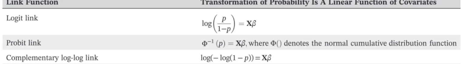
The regression coefficients from a Fine‐Gray subdistribution hazard model can be indirectly interpreted as the regres-sion coefficients for a complementary log‐log generalized linear model for the CIF similarly to hazard ratios without competing risks.7Three link functions are used with generalized linear models for binary outcomes: the logit link, the probit link, and the complementary log‐log link (see Table 1).
Of these 3, the logistic link function results in regression coefficients with which biostatistical analysts are the most familiar: odds ratios describing the relative effect of the covariates on the odds of the occurrence of the outcome. Unfor-tunately, regression coefficients from binomial regression models using the other 2 link functions are more challenging to interpret.9However, the sign of the regression coefficient (positive vs negative) provides information as to whether increases in the covariate are associated with an increase or decrease in the probability of the occurrence of the outcome. Thus, a positive regression coefficient indicates that a 1‐unit change in the variable is associated with an increase in the incidence of the outcome. However, the magnitude of a regression coefficient does not, on its own, provide information about the magnitude of the increase or decrease in the probability of the occurrence of the outcome over time. Instead, the estimated regression coefficients can be used to compute the probability of the occurrence of the event. As has been stressed previously, this holds true for the standard proportional hazards model in the absence of competing risks: The direction of the hazard ratio denotes the direction of the effect of a given covariate on incidence, but not the magnitude of the effect.
While the magnitude of the estimated regression coefficient does not provide information on the magnitude of the effect of the covariate on the incidence of the outcome, the fact that the coefficients can be seen as arising from a com-plementary log‐log model for the CIF does mean that one can make statements about the relative magnitudes of the effects of different covariates on the incidence of the same outcome (this is because, in the absence of competing risks, the log‐log model for the survival function of the event time results is a proportional hazards model for the hazard func-tion. A similar result can be established with competing risks when assuming a log‐log model for 1 − F1[where F1
denotes the CIF for events of type 1]. As the subdistribution hazard equals {dF1(t|X)/dt}/{1−F1(t|X)}, one may replace
the numerator and denominator with their equivalents under the log‐log model. Upon simplification, this yields a pro-portional hazards model for the subdistribution hazard, analogous to what is obtained in the absence of competing risks). If one covariate has a larger regression coefficient than that of a second covariate, then the magnitude of the effect of the first covariate on the incidence of the outcome will be greater than the magnitude of the effect of the second covar-iate on the incidence of the outcome (see Appendix A for derivation). Thus, in our case study, the hazard ratio for car-diovascular death for a 10‐year increase in age is 1.50, while the hazard ratio for males is 1.16. Thus, a 10‐year increase in age has a greater effect on the incidence of cardiovascular death than does male sex compared to female sex. Further-more, male sex is associated with an increase in the incidence of cardiovascular death that is equivalent to that associated with an increase in age of 3.6 years.
Unfortunately, one cannot make conclusions about the relative magnitudes of the effect of the same covariate on the incidence of different outcomes by comparing the relative magnitudes of the subdistribution hazard ratios. Since the baseline CIF differs between the different types of events, one is not able to conclude that because the subdistribution hazard ratio for a given covariate is larger in the first subdistribution hazard model than it is in the second subdistribution hazard model, that the effect of the covariate on the incidence of the first type of event is greater than on the incidence of the second type of event. In our empirical example, the subdistribution hazard ratio for a 10‐year increase in age was 1.50 for cardiovascular death and 1.20 for noncardiovascular death. However, we cannot infer that a 10‐year increase in age increases the incidence of cardiovascular death to a greater extent than it increases the incidence of noncardiovascular death. For similar reasons, a comparison of the relative magnitude of the subdistribution hazard ratios for the same type of event between different studies does not permit one to make conclusions about the relative magnitude of the effect of the covariate on the incidence of the outcome in the differ-ent studies.
TABLE 1 Generalized linear models for binary outcomes
Link Function Transformation of Probability Is A Linear Function of Covariates
Logit link
log p 1−p
¼Xβ
Probit link Φ−1ð Þ ¼p Xβ;whereΦðÞdenotes the normal cumulative distribution function
When the probability of an event is low, then the logistic link function and the complementary log‐log link function are very similar.9In particular, when the probability is less than 0.1, then these 2 link functions are almost indistinguish-able, while when the probability is between 0.1 and 0.2, differences between them are very small (Figure 1). Thus, in set-tings in which the probability of the occurrence of the event is low over meaningful durations of follow‐up, the coefficients from a subdistribution hazard model can be interpreted as odds ratios for the CIF. Thus, if the subdistribution hazard ratio is equal to 2, one can infer that a 1‐unit increase is associated with an approximate doubling of the odds of the occurrence of the event in settings in which the cumulative incidence of events is less than 0.20 over meaningful durations of follow‐up.
3
|
L I T E R A T U R E R E V I E W O F T H E U S E O F T H E F I N E
‐
G R A Y
S U B D I S T R I B U T I O N H A Z A R D M O D E L
In the previous section, we discussed the interpretation of regression coefficients from competing risk regression models. In this section, we report on a literature review that examined how authors in the medical literature interpreted the esti-mated coefficients from subdistribution hazard models. We searched the PubMed database (https://www.ncbi.nlm.nih. gov/pubmed) on November 1, 2016, using the following search strategy: (“subdistribution hazard”[All Fields] OR“Fine‐ Gray”[All Fields]) AND (“2015/01/01”[PDAT] :“2015/12/31”[PDAT]) to identify papers published in 2015 that used the Fine‐Gray subdistribution hazard model.
The search process identified 64 papers. Of these, we excluded 8 methodologically oriented publications and one additional paper because it did not use the Fine‐Gray subdistribution hazard model. We examined the remaining 55 papers to see how the authors interpreted the regression coefficients arising from the Fine‐Gray subdistribution hazard model.
Five (9%) papers interpreted the covariates as having an effect on the subdistribution hazard function. Strictly speak-ing, it is correct to infer that covariates with a regression coefficient that is statistically significantly different from zero have an effect on the subdistribution hazard function. However, as noted above, this interpretation may be nonintuitive or difficult for some to understand, as it describes the rate of the occurrence of events in subjects who have not yet expe-rienced the event of interest (but who may have expeexpe-rienced a competing event). Twenty‐four (44%) papers described the model covariates as having an effect on risk. While the term“risk”is often used without clarifying the meaning of the term, we interpret risk as meaning the probability of the occurrence of the event (cf. relative risk is the ratio of 2 prob-abilities). As noted previously, the direction of the effect of the covariate on risk (incidence) will be in the same direction as its effect on the subdistribution hazard function. However, the magnitude of the 2 effects need not coincide. Eleven (20%) papers described the covariates as having an effect on the incidence of the outcome. As stated previously, the subdistribution hazard model allows one to determine the effect of covariates on the CIF. However, as previously stated, the estimated hazard ratio determines the direction of the effect on incidence, but not the magnitude of the effect on
incidence. Seven (13%) papers described the covariates as having an effect on the rate of the outcome. This interpretation is correct only with a caveat: that one is determining the rate of the outcome in those subjects who have not experienced the given outcome (but who may have experienced a competing event and who thus contribute immortal time). If the focus is on rates, authors may be better served by using the cause‐specific hazard model, which models the effect of covariates on the rate of the outcome in subjects who are event‐free (and thus who have not experienced any type of event). Rates may be of greater interest when the study has an etiological focus, while risks may be of greater interest when the focus is on estimating patient prognosis and predicting patient outcome (eg, to inform the clinical management of patients).5Two papers (4%) described the covariates as having an effect on the time to the occurrence of the event.
When interpreting the numerical value of the estimated regression coefficients, 4 (7%) papers described it as denoting the relative increase in incidence due to the covariate. Thus, if the subdistribution hazard ratio was equal to 2, this was interpreted by the authors as meaning that the covariate was associated with a twofold increase in the incidence of the event. One (2%) paper made a similar interpretation about the magnitude of the effect of the covariate on the risk of the event. This is an incorrect interpretation of the magnitude of the subdistribution hazard ratio. The direction of the subdistribution hazard ratio describes the direction of the effect of the covariate on the risk or incidence of the outcome, but not the magnitude of this effect. When the event of interest is relatively infrequent, this subdistribution hazard ratio is approximately the effect on the risk of the event.
The subdistribution hazard model is also referred to as a CIF regression model because of the link between the subdistribution hazard and the effect on the incidence of the outcome. The reporting of a CIF provides context in which to interpret the direction of the estimated regression coefficients from the associated Fine‐Gray regression model. Because of this link, we examined whether studies that used the Fine‐Gray model also reported CIFs in the published paper. Of the 55 studies, 44 (80%) displayed at least one CIF curve.
4
|
D I S C U S S I O N
The Fine‐Gray subdistribution hazard model is increasingly being used for the analysis of time‐to‐event outcomes in the presence of competing events. The natural interpretation of the subdistribution hazard ratios arising from a fitted subdistribution hazard is the relative change in the subdistribution hazard function. Thus, the associated hazard ratios denote the relative change in therateof the occurrence of the events in subjects who have not yet experienced the event of interest (but who may have experienced a competing event). Due to the risk set containing subjects who have failed due to a competing event and whose continued existence in the risk set can be construed as representing“immortal time,”this interpretation may not appeal to some investigators and analysts.
We have highlighted that in the subdistribution hazard model, the covariates can be thought of as having an effect on the CIF. However, it is important to note that magnitude of the subdistribution hazard ratio does not, strictly speaking, convey the magnitude of the effect of the covariate on the CIF. This error in interpretation appears to occur moderately frequently in the medical literature. In a study examining cardiovascular disease risk in a cohort of breast cancer survi-vors, the authors estimated a subdistribution hazard ratio of 1.19 for the comparison of right‐sided radiation therapy compared to left‐sided radiation therapy after mastectomy.10The authors interpreted this as right‐sided radiation ther-apy increasing the cumulative incidence 1.19‐fold (p 1066), which is only approximately correct. Similarly, in a study examining the effect of hyponatremia on the incidence of cardiovascular events in peritoneal dialysis patients, the authors estimated a subdistribution hazard ratio of 2.31.11The authors interpreted this as meaning that patients with hyponatremia had a 2.31‐fold higher risk of cardiovascular events (p 4/10). Similar examples can be found elsewhere in the literature.12-14We suggest that when reporting the effect of a covariate on the incidence of the primary outcome, that the analyst and authors either restrict themselves to discussing the direction of the effect or be careful to note that the quantification of the magnitude of the effect on the cumulative incidence is only approximately correct using the subdistribution hazard ratios.
The current review was based on published articles that reported the use of a Fine‐Gray subdistribution hazard regression model. We focused on how authors interpreted the hazard ratios associated with this regression model. We would like to stress that the presence of competing risks does not automatically imply that the Fine‐Gray subdistribution hazard model is the most appropriate regression model. Lau et al suggest that there are 2 broad rationales for fitting a regression model: The first is for etiological reasons (eg, is a given risk factor or characteristic associated with the rate of the occurrence of the outcome in subjects who are currently event‐free), while the second is for prognostic reasons (eg, what is an individual's probability of experiencing the outcome within a given duration of time).5Lau et al suggest that the cause‐specific hazard model is more appropriate for addressing etiological questions, while the Fine‐Gray model is more appropriate for addressing questions around incidence and prognosis. Both we and Wolbers et al have echoed this assertion.4,15Thus, if the research objective is to derive a model for predicting the probability of the occurrence of outcomes over time, then a subdistribution hazard model would be appropriate.16,17Failure to use the Fine‐Gray model for such a research objective can result in estimates of the probability of the occurrence of the outcome that are biased upwards.17 When analyzing survival data in which competing risks are present, rather than beginning with a predetermined type of regression model, the investigator and analyst should begin by carefully formulating the research question and then selecting the model that is most appropriate for addressing the formulated question. In many instances, particularly in epidemiological research, the most appropriate model will be the cause‐specific hazard model. However, in settings in which it is important to make inferences about the effect of covariates on the incidence of the outcome, then the Fine‐Gray model will be the most appropriate model. Some authors have suggested that to develop a greater understanding of the relationship between covariates and outcomes, that both cause‐specific and subdistribution hazard models be fit, for both the primary outcome and for the competing events.8When doing so, the principal message of the current study is that the regression coefficients from the subdistribution hazard model must be interpreted correctly.
We recently published a review of how competing risks were addressed in reports of randomized controlled trials (RCTs) published in 4 leading general medical journals.18In this previous review, we estimated that 77.5% of RCTs with a time‐to‐event outcome were potentially susceptible to competing risks. Amongst those studies that were potentially susceptible to competing risks, we examined whether the statistical methods used were appropriate for the analysis of competing risks survival data. We found that of those studies potentially susceptible to competing risks, 77.4% reported the results of a Kaplan‐Meier survival analysis, while only 16.1% reported using CIFs to estimate the incidence of the outcome over time in the presence of competing risks. We concluded our previous review of reported analyses in RCTs with recommendations for analyzing RCTs in the presence of competing risks. The objective of the current review is dif-ferent from that of our earlier review. The focus of the current review was to examine how authors interpreted the haz-ard ratios arising from a Fine‐Gray subdistribution hazard model. We were not interested in the appropriateness of the fitted model, but rather in how the resultant model was interpreted. As such, the current article makes the important distinction between rates and risks or probabilities.
The key message of this paper for applied analysts and clinical researchers is that there is not an exact link between the subdistribution hazard ratio and relative changes in the CIF except for settings in which the event of interest is rare. The direction of the subdistribution hazard ratio denotes the direction but does not directly provide the magnitude of the effect of the covariate on the CIF. Care is needed when attempting to make statements about the magnitude of the covar-iate effects on the CIF using the subdistribution hazard ratios, as such statements are at best only approximately correct. Furthermore, the relative magnitudes of different covariates from the same subdistribution hazard model allow one to make inferences about the relative magnitudes of the effects of the covariates on the incidence of the given type of event.
F U N D I N G S O U R C E S
O R C I D
Peter C. Austin http://orcid.org/0000-0003-3337-233X
R E F E R E N C E S
1. Kaplan EL, Meier P. Nonparametric estimation from incomplete observations.J Am Stat Assoc. 1958;53:457‐481. 2. Cox D. Regression models and life tables (with discussion).J Royal Stat Soc‐Series B. 1972;34:187‐220.
3. Tu JV, Donovan LR, Lee DS, et al. Effectiveness of public report cards for improving the quality of cardiac care: the EFFECT study: a ran-domized trial.JAMA. 2009;302(21):2330‐2337.
4. Austin PC, Lee DS, Fine JP. Introduction to the analysis of survival data in the presence of competing risks.Circulation. 2016;133:601‐609. https://doi.org/10.1161/CIRCULATIONAHA
5. Lau B, Cole SR, Gange SJ. Competing risk regression models for epidemiologic data.Am J Epidemiol. 2009;170(2):244‐256. https://doi.org/ 10.1093/aje/kwp107
6. Putter H, Fiocco M, Geskus RB. Tutorial in biostatistics: competing risks and multi‐state models.Stat Med. 2007;26(11):2389‐2430. https:// doi.org/10.1002/sim.2712
7. Fine JP, Gray RJ. A proportional hazards model for the subdistribution of a competing risk.J Am Stat Assoc. 1999;94:496‐509.
8. Latouche A, Allignol A, Beyersmann J, Labopin M, Fine JP. A competing risks analysis should report results on all cause‐specific hazards and cumulative incidence functions.J Clin Epidemiol. 2013;66(6):648‐653.
9. McCullagh N, Nelder JA.Generalized Linear Models. London: Chapman & Hall; 1989.
10. Boekel NB, Schaapveld M, Gietema JA, et al. Cardiovascular disease risk in a large, population‐based cohort of breast cancer survivors.Int J Radiat Oncol Biol Phys. 2016;94(5):1061‐1072. https://doi.org/10.1016/j.ijrobp.2015.11.040
11. Kim HW, Ryu GW, Park CH, et al. Hyponatremia predicts new‐onset cardiovascular events in peritoneal dialysis patients.PLoS One. 2015;10(6): e0129480. DOI: https://doi.org/10.1371/journal.pone.0129480
12. Han K, Pintilie M, Lipscombe LL, Lega IC, Milosevic MF, Fyles AW. Association between metformin use and mortality after cervical can-cer in older women with diabetes.Cancer Epidemiol Biomarkers Prev. 2016;25(3):507‐512. https://doi.org/10.1158/1055‐9965.EPI‐15‐1008 13. Bai AD, Showler A, Burry L, et al. Impact of infectious disease consultation on quality of care, mortality, and length of stay in Staphylo-coccus aureus bacteremia: results from a large multicenter cohort study.Clin Infect Dis. 2015;60(10):1451‐1461. https://doi.org/10.1093/ cid/civ120
14. Feinstein L, Edmonds A, Okitolonda V, et al. Implementation and operational research: maternal combination antiretroviral therapy is associated with improved retention of HIV‐exposed infants in Kinshasa, Democratic Republic of Congo.J Acquir Immune Defic Syndr. 2015;69(3):e93‐e99. https://doi.org/10.1097/QAI.0000000000000644
15. Wolbers M, Koller MT, Stel VS, et al. Competing risks analyses: objectives and approaches.Eur Heart J. 2014;35(42):2936‐2941. https://doi. org/10.1093/eurheartj/ehu131
16. Austin PC, Lee DS, D'Agostino RB, Fine JP. Developing points‐based risk‐scoring systems in the presence of competing risks.Stat Med. 2016;35(22):4056‐4072. https://doi.org/10.1002/sim.6994
17. Wolbers M, Koller MT, Witteman JC, Steyerberg EW. Prognostic models with competing risks: methods and application to coronary risk prediction.Epidemiology. 2009;20(4):555‐561.
18. Austin PC, Fine JP. Accounting for competing risks in randomized controlled trials: a review and recommendations for improvement.Stat Med. 2017;36(8):1203‐1209. https://doi.org/10.1002/sim.7215
How to cite this article: Austin PC, Fine JP. Practical recommendations for reporting Fine‐Gray model analyses
for competing risk data.Statistics in Medicine. 2017;36:4391–4400.https://doi.org/10.1002/sim.7501
A P P E N D I X A
C O M P L E M E N T A R Y L O G‐L O G M O D E L F O R T H E C I F—R E L A T I V E E F F E C T S O F D I F F E R E N T
C O V A R I A T E S
Let us assume that we have a complementary log‐log model for the CIF with 2 covariates:
log(−log(1−p)) =α0+α1X1+α2X2, wherepdenotes the probability that the event of interest occurs prior to timet
Then we have that
−log 1ð −pÞ ¼eα0þα1X1þα2X2;
log 1ð −pÞ ¼−eα0þα1X1þα2X2 ¼−eα0eα1X1eα2X2;
1−p¼e−eα0eα1X1eα2X2
; p¼1−e−eα0eα1X1eα2X2
:
The above probability of the event occurring prior to timetis conditional onX1andX2.
The probability of the event occurring given thatX1=x1+ 1 is equal to
p∣x1þ1;x2¼1−e−e
α0eα1ðx1þ1Þeα2x2
¼1−e−eα0eα1x1eα1eα2x2
.
The relative incidence of the event prior to timetfor a subject withX1=x1+ 1 compared to a subject withX1=x1(but
holdingX2fixed atx2) is equal to
1−e−eα0eα1x1eα1eα2x2
1−e−eα0eα1x1eα2x2 ¼
1− e−eα0eα1x1eα2x2eα1
1−e−eα0eα1x1eα2x2 .
We replace the common term in the numerator and denominator byBfor simplicity. Thus, we have that the relative
incidence is equal to1−B
eα1
1−B . Now, the quantity in the denominator is a probability and is thus between 0 and 1. There-fore, we have thatBis also between 0 and 1.
Similarly, the relative incidence of the event prior to timetfor a subject withX2=x2+ 1 compared to a subject with
X2=x2(but holdingX1fixed atx1) is equal to
1−Beα2
1−B .
Now, if the regression coefficient forX1is greater than the regression coefficient forX2, we have that
α1>α2
eα1>eα2ðsince the exponential function is an increasing functionÞ
Beα1
<Beα2ðsince B is between 0 and 1;the direction of the inequality changesÞ
−Beα1
>−Beα2 1−Beα1
>1−Beα2
1−Beα1 1−B >
1−Beα2 1−B :
Thus, if the first regression coefficient is larger than the second regression coefficient, the relative change in the inci-dence of the outcome associated with a 1‐unit change inX1is greater than the relative change in the incidence of the
![FIGURE 1 Comparison of logit and complementary log ‐log link functions [Colour figure can be viewed at wileyonlinelibrary.com]](https://thumb-us.123doks.com/thumbv2/123dok_us/8255949.2187378/6.892.86.555.767.1088/figure-comparison-complementary-functions-colour-figure-viewed-wileyonlinelibrary.webp)
