4879.pdf

(1)

Polarized Photofission Fragment Angular

Distributions of

232

Th and

238

U

Jeromy Ryan Tompkins

A dissertation submitted to the faculty of the University of North Carolina at Chapel Hill in partial fulfillment of the requirements for the degree of Doctor of Philosophy in the Department of Physics and Astronomy.

Chapel Hill 2012

Approved by:

H. J. Karwowski

M. W. Ahmed

T. B. Clegg

(2)

c O 2012

(3)

ABSTRACT

JEROMY RYAN TOMPKINS: Polarized Photofission Fragment Angular Distributions of 232_{Th and} 238_U.

(Under the direction of H. J. Karwowski.)

A study of photofission fragment angular distributions on 232_{Th and} 238_{U has been}

completed for the first time using linearly-polarized, quasi-monoenergetic photon beams of near-barrier energies. Large polarization asymmetries are observed in both nuclei. For232_{Th, fragments are emitted in the direction of beam polarization with more than}

fifteen times greater preference than perpendicular to it when the beam energy is 6.2 MeV. These asymmetries are roughly a factor of two times greater than are character-istic of238_{U. The large observed fragment asymmetries are responsible for asymmetries}

(4)

List of Tables

3.1 Fission channel angular distributions . . . 24

4.1 Table of previous measurements . . . 35

5.1 Characteristics of photon beams . . . 52

5.2 Target characteristics . . . 56

6.1 Four-point calibration alpha decays . . . 74

7.1 Geometrical adjustments in robustness investigation . . . 93

8.1 Tabulated results . . . 95

C.1 Angular positions - 232_{Th . . . .} ₁₁₆

(9)

List of Figures

2.1 Mass yield curve for 238U . . . 6

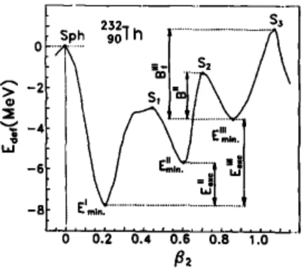
2.2 Potential energy surface for 232_{Th . . . .} ₁₂

2.3 Triple humped barrier . . . 13

2.4 Schematic multihumped barrier . . . 14

3.1 Euler angles . . . 20

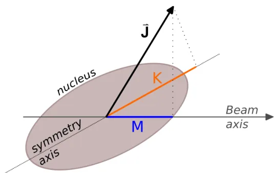
3.2 Definition of J,K, and M . . . 21

3.3 Schematic collective excitation level scheme . . . 23

4.1 b/a of 238U . . . 38

4.2 b/a of 232_{Th - bremsstrahlung sources . . . .} ₃₉

4.3 Comparison of b/a between 238U and 232Th . . . 40

4.4 c/b of 238_{U - bremsstrahlung sources . . . .} ₄₃

4.5 c/b of 232_{Th - bremsstrahlung sources . . . .} ₄₄

4.6 Diagram of multihumped barrier with different channels . . . 46

(10)

5.4 Electronics block diagram . . . 59

5.5 Block diagram of the full circuit . . . 60

5.6 Beam energy measurement . . . 66

5.7 Geant4 detector geometry . . . 67

6.1 Analysis diagram . . . 69

6.2 ADC spectrum . . . 72

6.3 232_{Th alpha partice spectrum} _{. . . .} ₇₃

6.4 232_{Th fragment yield ratios . . . .} ₇₈

6.5 232Th fragment yield ratios . . . 79

7.1 Optimization adjustments in Geant4 model . . . 85

7.2 Optimized relative geometry comparison . . . 86

7.3 Marginal η function . . . 88

7.4 h24 probability function . . . 90

7.5 Comparison of alpha particle range . . . 92

7.6 Comparison of alpha particle angular straggling . . . 93

8.1 Polarization asymmetry of 232_{Th . . . .} ₉₆

8.2 θ asymmetry of 232_{Th . . . .} ₉₇

8.3 Comparison of 232Th b/a to previous data . . . 98

8.4 Theta-dependent asymmetry comparison - 232_{Th . . . .} ₉₉

8.5 c40 trend of 232Th . . . 100

(11)

8.6 Comparison of polarization asymmetry between 238_{U and} 232_Th _{. . . .} ₁₀₃

(12)

List of Abbreviations

ADC Analog-to-digital converter BPM Beam pickoff monitor

CEBAF Continuous Electron Beam Accelerator Facility CODA CEBAF Online Data Acquisition system CFD Constant-fraction discriminator

DAQ Data acquisition system FAD Fragment angular distribution FEL Free electron laser

HPGe High-purity germanium HIγS High Intensityγ-ray Source GDR Giant dipole resonance

GS Ground state

JLAB Thomas Jefferson National Accelerator Facility

LD Liquid drop

LDM Liquid drop model

LED Leading-edge discriminator LTF Live time fraction

NAD Neutron angular distribution

PFAD Photofission fragment angular distribution

(13)

SSD Silicon strip detector TDC Time-to-digital converter TKE Total kinetic energy TOF Time of flight

(14)

Chapter 1 Introduction

1.1 The Importance of Fission

Few people in the world have never heard the word “fission”, and for good reason. Fission has shaped the twentieth and twenty-first centuries in ways that no other nu-clear reaction has. It has influenced the world both politically and economically. It has ended wars and nearly begun others. In light of this, one might believe that fission is well understood. To say so, is to be partially correct. It is also to sweep under the rug lots of unsolved questions that have attracted the attention of subatomic physicists since the early days of its discovery. Fission is richly complicated. An understanding of observables resulting from fission requires information of both static nuclear properties, large-scale nuclear dynamics, understanding of nuclear configurations in extreme con-ditions, and the respective strengths of collective and single-particle degrees of freedom [2].

(15)

micro-scopic description tenable. An improved understanding of fission not only is satisfying from a scientific perspective but also from a practical perspective. It is expected to im-prove future nuclear reactor designs and understand their performance characteristics; current reactors are operated well below maximum power output because the limits of safe operation are not well established. Such an improved understanding would directly impact the power output of existing reactors and increase their safety.

1.2 The Discovery of Fission

Fission was first observed by E. Fermi and coworkers in 1934 as they were seeking to create transuranic elements by β-decay that follows neutron capture [4, 5]. They observed that following activation by neutrons, radioactive species of 4 half-lives were produced, some of which were not identifiable with elements known at the time. For this reason, they claimed that elements beyond uranium had been discovered. Their results were questioned by many and a series of experiments followed by multiple in-dependent research groups [6]. The culmination of these efforts was the experimental determination by Hahn and Strassman that elements of medium mass, such as Ba, were produced by neutron bombardment of uranium [7]. Otto Hahn was subsequently awarded the Nobel Prize in 1944 for the discovery of fission.

(16)

to release ≈ 200 MeV [8]. Frisch was able to detect these high energy fragments with a uranium-lined ionization chamber and a neutron source. This further corroborated the presence of a large scale splitting in the nucleus [9].

Following this striking evidence and other experiments that confirmed this new reaction, the ground work was laid for the understanding of fission in the viewpoint of the liquid drop model by Bohr and Wheeler [10]. The qualitative understanding that these scientists brought about has largely persisted to this day.

1.3 Overview of Contents

In the present work, the fission of238U and232Th following the absorption of linearly-polarized photons with energies, Eγ, between 5.7 MeV and 7.6 MeV was investigated.

This document will motivate and discuss a measurement of the angular distributions of fission fragments from photon-induced fission reactions.

To provide a context for these studies, fission as a whole will be discussed in Ch. 2. Within this chapter, the general characteristics of fission and the present understanding will be presented. Also, fission induced by photons, photofission, is a subfield of fission research that is most relevant to this work. For this reason, its general features will be explained as well.

A more specific discussion on the angular distributions of fission fragments from photofission will follow in Ch. 3. Two paradigms by which fission fragment angular distributions are understood will be presented. A review of all the measurements of

(17)

238_{U and} 232_{Th photofission fragment angular distributions (PFADs) is included as}

Ch. 4. Since measurements have focused on a large variety of topics, the discussion has been organized by major physics findings.

A related project seeking to understand prompt-fission neutron angular distributions has provided the ultimate impetus for these studies. Its findings are important to understand the reason the present project has been undertaken. Therefore, a concise description of the experiment and its results are included in Ch. 5. It will be followed by the detailed description of the experimental setup of the PFAD experiment that is the topic of this paper. With knowledge of the experimental setup, the reader will be introduced to the characteristics of the acquired data.

(18)

Chapter 2 Fission Theory

2.1 General Fission Characteristics

(19)

energy release of up to 200 MeV accompanies each fission event that is largely the result of Coulomb energy release. The released energy is split between the total kinetic energy of the fragments and their internal excitation energies so that the fragments are highly excited following scission. Because they are also neutron rich, relaxation is most efficiently accomplished by the emission of neutrons and subsequently photons. More exotic fission events do occur, such as ternary fission when three particles result rather than two, but the remainder of this document will consider the binary fission process described above.

Nuclear Mass

80

100

120

140

160 Y

ie

ld

%

0

1

2

3

4

5

6

7 U Mass Yield Curve

238

Figure 2.1: The asymmetric mass yield curve for 238_{U [11]. The preference to fission}

(20)

2.2 Photofission

Fission is believed to begin with the formation of a compound nucleus, that is, an ex-cited nucleus for which the excitation energy has been shared between all single-particle states in a complex way. A compound nucleus can be produced through a variety of excitation mechanisms, each with its own peculiarities. Particle-bombardment is one such means and tends to produce an initial nucleus with high angular momentum and energy. For this reason, particle-induced fission is useful for studying a regime of fission that is either minimally sensitive to the shell structure of the nucleus or involves high angular momentum. The use of photons, on the other hand, preferentially produces low-spin configurations at all energies. The benefit of a low spin is that the complexity of the reaction is reduced. Extraction of information from the reaction is therefore less complicated and can be potentially understood better. Fission induced by pho-tons, photofission, is therefore a useful method for investigating the low-energy regime, which is the most important for practical applications.

2.2.1 Key Characteristics of Photoabsorption

The interaction of electromagnetic fields, i.e. photons, and matter is considered the most well understood interaction in nuclear physics. Two of its main results are included here. A more detailed derivation is included in Appendix A for completeness. The first is a selection rule. It states that an electromagnetic field of multipolaritylcan couple an initial state with angular momentaJi to a final state with angular momentum

(21)

Jf if the triangle rule|Ji−l| ≤Jf ≤Ji+l is satisfied. Further, the associated transition

rate, Tf i, is given by [12]

Tf i(l; Π) =

8π(l+ 1)

l[(2l+ 1)!!]

k2l+1

~

|hf|Ωˆlµ(Π)|ii|2, (2.1)

where Π denotes whether the transition is electric or magnetic in nature and the matrix element contains all of the information regarding the nuclear wavefunctions.

With these results, it is possible to understand the benefits of photon absorption as the mechanism for inducing fission in even-even nuclei. Without considering the magnitude of the matrix element, Eq. 2.1 indicates that for a fixed k value, which is proportional to photon energy, the transition rate decreases rapidly as l increases. If this fact is coupled with the selection rules, an even-even nucleus in its ground state J = 0 will be excited to states of J = 1 or J = 2. Continuing to ignore the contribution of the nuclear matrix element, the energy dependence of these rates is weak as elicited by the fact that k = Eγ/197 MeV fm. As compared to other

(22)

2.3 Theoretical Overview

Though the ideas presented at the outset of fission research, such as the liquid drop model, are still integral to the manner in which fission is understood today, insights to the process have been provided by new approaches to study the process and the advent of modern computing power. Today, fission is better understood, but there are still fundamental observations, such as the mass yield distribution, that are not universally predictable.

The extent to which fission is understood is made clear by a survey of the theo-retical calculations. There are two categories that all calculations fall into: those that treat fission as a dynamical process and those that do not. An excellent example of the static description of fission is the macroscopic-microscopic model that will be pre-sented in Sect. 2.3.1. The original form of this hybrid model was able to predict a more complicated fission barrier structure, and variations of it have proven fruitful in understanding experimental observations. Another static approach uses the statistical model to calculate observables such as mass yields and angular distributions and will be discussed briefly in Sect. 2.3.2. Dynamical calculations require the most detail and will be summarized in section 2.3.3. The following discussion does not attempt to be exhaustive and merely serves to overview the current understanding of fission so the reader can grasp one simple point: fission is only partially understood and requires further theoretical and experimental effort.

(23)

2.3.1 Macroscopic-Microscopic Calculations

The first theoretical approach is an extended form of the original fission theory de-rived by Bohr and Wheeler [10]. It computes the energy of the nucleus for deformed shapes classically and then adds corrections to account for the quantum mechanical na-ture of the nucleus. This approach was successfully applied to fission first by Strutinsky [14] and its results were largely successful in removing the large discrepancies between the classical treatment and the observations.

The classical description of the nucleus is that of a uniformly-charged liquid drop (LD) with a sharp edge, as was first proposed by Bethe and Weizsacker [15, 16], ex-tended by Meitner and Frisch [8], and then fleshed out by Bohr and Wheeler [10]. In such a description, the energy can be computed for a given nuclear shape which is parameterized by a polynomial expansion,

R(θ, φ) = R0

λ

X

l l

X

m=−l

βlmYlm(θ, φ), (2.2)

whereλ is a scale factor to ensure volume conservation, βlm is the coefficient of thelth

multipole in the expansion, and Ylm is a spherical harmonic. The energy of such a LD

is made up of three contributing terms referring to the volumeEV, surface tensionES,

(24)

Since these calculations are concerned with deviations of the shape from a sphere, it is natural to discuss the difference in energy between the deformed nucleus and the spherical nucleus. Since only the ES and EC depend on the deformation, they alone

contribute to this difference. For small deformations, the shape is sufficiently described by an expansion of the surface up to quadrupole terms and the restoring force Fr is

obtained by the derivative of this energy, given as [17]

Fr =−

dE dβlm

=−ES(0)

1

4π(l−1)(l+ 2)−x

5

π l−1 2l+ 1

βlm. (2.4)

Here x is the fissility parameter defined as x = EC(0)/2ES(0) ∝ Z2/A where ES(0)

indicates the surface energy for zero deformation. The first term is the contribution of the surface energy and the second the Coulomb energy. Note that the surface term contributes a restoring force whereas the Coulomb term is a repulsive force. Equa-tion (2.4) shows that for the case of small quadrupole deformaEqua-tions the force becomes repulsive when x >1, and the LD becomes unstable to quadrupole deformations. The splitting of the drop is then energetically possible.

Further, the potential energy of the LD when plotted in parameter space βlm

con-tains a saddle point, see Fig. 2.2, which is referred to as the fission barrier. The model has been improved in recent years by considering additional terms to the energy [19] and is comparable, if not better than, microscopic calculations. However, such a model does not predict some known features of fission, such as fission isomers.

It is no surprise that the LD model fails to give an exact description of fission,

(25)

Figure 2.2: The potential energy landscape calculated for232_{Th. The potential energy}

is plotted as a function of the dipole,β2, and quadrupole, β3, deformation parameters.

Three minima are present. The figure has been taken from Ref. [18].

(26)

Figure 2.3: A schematic of the a multi-humped potential energy surface. Three saddle points are separated by two potential wells. Each of these has associated with it its own system of energy levels. Figure has been taken from Ref. [18].

2.3.2 Statistical Fission Calculations

The benefit of the dynamical fission calculations is their ability to calculate observ-ables such as the mass distribution. The source of their power is the detail to which they treat the fission process. However, the detail comes at a cost. They rely upon knowledge of the transport parameters such as the inertial mass and friction tensors,

(27)

β

E

n

er

gy

(

MeV

)

A

GS

B

C

0

6 LDM

_LDM

+

sc

I

II

III

Figure 2.4: A schematic view of a triple-humped fission barrier. Three potential wells exist labeled I, II, and III that are separated from each other by three saddle points A, B, and C. The first well contains the true ground state GS. The potential energy calculated in the liquid drop model is drawn as a dashed curve. The solid curve is the barrier predicted by a macroscopic-microscopic calculation. It includes shell-model cor-rections to the liquid drop energy and is labeled LDM+sc. Since multiple deformation parameters describe the nuclear shape, often 5, the potential energy is a hypersurface. The above is representative of the potential energy along a “valley” in the hypersur-face. The abscissa β represents the set of deformation parameters at any point along the fission path depicted.

(28)

Ref. [17] and will not be repeated here.

2.3.3 Fission Dynamics

Two general approaches to compute fission dynamics have been followed. The distinguishing assumptions of each are such that they apply to conditions that are orthogonal to each other. As a result, there is no potential for calculating the same observable reliably with both approaches. However, they both make the assumption that the shape of the nucleus can be parameterized when it transitions continuously from the initial compound nucleus into fission fragments. Interestingly, it has been pointed out that no conclusive evidence to support this exists in spectroscopic data [17]. Regardless of the accuracy of this approximation, the concept of continuous transitions between highly-deformed shapes is useful. Often the descent from saddle to scission is the subject of these calculations because it is expected to be the most important for determining quantities such as the sharing of the partition of the energy between kinetic and internal excitation and mass yields.

The first general approach treats the process adiabatically. It therefore assumes that such an extreme transition in the nucleus occurs in a manner that allows the nucleus to remain in the configuration defined by the lowest energy single particle levels. The energy of the system is, therefore, carried solely by the shape degrees of freedom. In fission calculations, this approximation is equivalent to the absence of frictional damp-ing durdamp-ing deformation. The second general approach treats an alternative extreme. It assumes that the energies involved in the fission event are high enough that the process

(29)

can be treated in a classical sense.

(30)

Chapter 3 Fission Fragment Angular

Distributions

One of the important subjects of photofission studies has been the fragment angular distributions, W(θ), that are associated with even-even nuclei. Anisotropies in the photofission of 232Th were discovered by Winhold, Demos, and Halpern [24] in 1952. They were able to fit the angular distribution with the function

W(θ) =a+bsin2θ (3.1)

(31)

puzzled to learn that the anisotropy disappeared as the photon energy was increased to energies of the GDR region, Eγ = 10 - 20 MeV. It was obvious then that the origin

of the anisotropy was different than that of the GDR. It was not until 1956 that A. Bohr [26] presented a satisfactory explanation for their results.

Bohr’s explanation has remained at the heart of the present understanding of fission fragment angular distributions (FADs), though it was extended to include fission in-duced by polarized photons. On the other hand, recent insights and a new approach to understanding the FADs, hereafter referred to as the Kadmensky approach, has been derived by Kadmensky and collaborators [27]. The form of the angular distribution derived by each of these models is nearly identical but the steps and assumptions em-ployed to arrive at the result are sufficiently different to warrant separate discussions. The channel formalism based on Bohr’s ideas in Sect. 3.1 will be followed by that of Kadmensky in Sect. 3.2. Both of these concern the angular distribution that might arise from a single transition state. Because a fission path typically involves the transition through at least two saddle points, some comments on the effect of multiple saddles to the presented theories will be given in Sect. 3.4. For completeness, an account of the previous measurements for photofission FADs (PFADs) will follow in Chapter 4.

(32)

angular distribution, W(θ, φ), can be described by

W(θ, φ) = a+bsin2θ+csin22θ+ωPγ

dsin2θ+csin22θ (3.2)

if dipole and quadrupole absorption are considered. In Eq. 3.2, the ω is +1(-1) for transitions that are electric(magnetic) in nature. It is important to understand that the formalism ignores the dynamics of the fission process prior to the saddle point except to assume that it is adiabatic.

Two crucial assumptions are made in the treatment. The first is that the transition states of the fissioning nucleus correspond to collective rotations, and the second is that the associated nuclear shape is axially symmetric. Given these, the wavefunction should be the same as that of the symmetric top, otherwise known as the symmetric rotor. The Hamiltonian for the symmetric rotor, in a purely collective model, is

ˆ

H= ˆJ

02₋_ˆ_J02

z

2Ω , (3.3)

where the primed operators are the body-fixed angular momentum operators and Ω is the moment of inertia for rotations about the symmetry axis. Such a Hamiltonian is diagonalized by wavefunctions of the form

φJ_{M K}(ω) =DJ

M K(ω), (3.4)

where theDJ

M K(ω) are rotation matrix elements corresponding to rotations about the

(33)

x

x'

y'

y

ϕ

x

_x'

y

y'

z'

z

θ

x

x'

x''

y

y'

y''

z

z'

γ

Figure 3.1: Diagram of the Euler angles that define the orientation of a body in three-dimensional space. The rotations are ordered as illustrated by proceeding clockwise from the top left. For an axially-symmetric nucleus, the first two rotations φ and θ

define the orientation of the symmetry axis with respect to the laboratory frame.

(34)

J

M

K

sym

met

ry

axis

Beam

axis

Figure 3.2: TheJ,K, andM quantum numbers that define the orientation of the body-fixed coordinate system of the axially-symmetric nucleus with respect to the laboratory coordinate system. This definition fixes the nuclear symmetry axis to the z-axis of the body-fixed frame and the beam axis to the z-axis of the laboratory.

where thedJ

M,K functions are the Wigner rotationald-functions. The lowest order forms

of these functions are listed in Section B.1. Their explicit form is [28]

dJ_M,K(θ) =p(J+M)!(J −M)!(J+K)!(J−K)!

×X

M0

(−1)M0[sin(θ/2)]2M0−M+K[cos(θ/2)]2J−K+M−2M0 (J−K−M0_)!(_J₊_M₋_M0_)!(_M0₊_K₋_M_)!(_M0_)!,

(3.6)

where the summation is over allM0 for which the terms in the denominator are greater than or equal to zero. If one further assumes that the transition of the system from saddle to scission is characterized by the separation of the fragments along the nuclear

(35)

symmetry axis and that the orientation of this axis is fixed in space, i.e.,K is conserved, then the angular distribution for unpolarized photons should be simply the square of these matrix elements,

W_{M K}J (θ)∝ |dJ_{M K}(θ)|2_. _(3.7)

The present experiment is unable to distinguish the helicity of the photon that caused the fission event. For this reason, the M = ±1 states are summed over to create a channel distribution dependent on J and K only,

W_KJ(θ, φ) = 2J + 1 2

1 2

|dJ₁_,K(θ)|2 +|dJ−1,K(θ)|

2

. (3.8)

If the photon beam is polarized to a fractional value, Pγ, the rotational symmetry

about the beam axis is broken. The similar expression for Eq. 3.8 when polarization is present is [29]

W_KJ(θ, φ) = 2J+ 1 2

1 2

|dJ₁_,K(θ)|2+|dJ₋₁_,K(θ)|2

−ωPγcos 2φdJ1,K(θ)d J

−1,K(θ)

. (3.9)

(36)

in Ref. [30].

0+

2+

6+

4+

K=0

3-

1-

5-

7-K=0

2+

1+

3+

4+

K=1

Gr

ound

s

tat

e

M

as

s-

asy

m

met

ry

Be

nd

in

g

E

ne

rg

y

Figure 3.3: A schematic level scheme of a heavy nucleus as presented in Ref. [30]. States that are expected to contribute to dipole fission are colored red and those for quadrupole fission green.

The measured angular distribution is generated by the linear combination of these channel angular distributions. Recall that in Sect. 2.2.1 it was demonstrated that the absorption of a photon will excite an even-even nucleus in the ground state primarily to states of Jπ = 1− and occasionally to Jπ = 1+ or 2+, if the nuclear wavefunction does not bias the probability toward other states. Bohr argued that the excitation spectrum of the fissioning nucleus would be similar to the states in the first potential well despite the fact that the nucleus at the transition state should be sufficiently different. These are characterized by rotational and vibrational bands with different

(37)

K values and parities, see Fig. 3.3. If this assumption is correct, the minimum energy level at the saddle point would likely be a 0+ _{state followed by a 2}+ _{state in the same}

rotational band with K = 0. The next state would then be the 1− state of a K = 0 band with negative parity. If the fissioning nucleus has an excitation spectrum of this form, then the nucleus will preferentially absorb the photon through E1, M1, and E2 transitions. The measured angular distribution would then be reasonably well modeled by the combined channel distributions of all dipole and quadrupole terms.

J K Channel Coeff WJ

K(θ)

1 0 x 3₄sin2θ+ 3₄ωPγcos 2φsin2θ

1 ±1 y 3₄ 1− 1

2sin 2_θ

− 3

8ωPγcos 2φsin 2_θ

2 0 u 15₁₆sin22θ+ 15₁₆ωPγcos 2φsin22θ

2 ±1 v 5₈ 2−sin2θ−sin22θ+5₈ωPγcos 2φ sin2θ−sin22θ

2 ±2 w 5₈ sin2θ+ 1₄sin22θ− 5

8ωPγcos 2φ sin 2_θ₋ 1

4sin 2₂_θ

Table 3.1: The angular distributions of specific fission channels derived from Eq. 3.9. It is implied that M =±1 has been averaged over.

The channel wave functions for the contributing dipole and quadrupole terms are listed in Table 3.1. If one includes all dipole and quadrupole channels and then collects like terms, the total angular distribution becomes [29, 30]

W(θ, φ) = a+bsin2θ+csin22θ+ωPγ

dsin2θ+csin22θ). (3.10)

(38)

±1), and (J = 2, K = ±2). The a, b, c, and d coefficients can be decomposed into these channels clearly by defining a matrix A that combines the channel contributions

ζ = (x, y, u, v, w) into the angular distribution parameters p = (a, b, c, d) by p = Aζ. The conversion matrix is

A=            

0 3/2 0 5/2 0

3/4 -3/4 0 -5/4 5/4 0 0 15/16 -5/4 5/16 -3/4 3/4 0 -5/4 5/4

            . (3.11)

In the literature, there is little agreement as to the proper way to represent the angular distribution. Equation 3.10 is the convention chosen for the present work because of the consistency of thecterms. Another common form for the polarized angular distribution is presented by Ratzek and collaborators [30] as

W(θ, φ) = a+bsin2θ+csin22θ+ωPγcos 2φ

dsin2θ−4csin4θ. (3.12)

Their preferred form of the angular distribution differs from Eq. 3.10 by the definition ofd. One can convert from Eq. 3.10 to Eq. 3.12 by defining thedparameter of Eq. 3.12 in terms of the coefficients of Eq. 3.11 such that dRatzek →d+ 4c.

(39)

3.2 The Kadmensky Fragment Angular

Distribu-tion

The approach of Kadmensky and collaborators, developed in a series of papers [23, 27, 31, 32], is based on similar concepts to Bohr’s theory but addresses the uncertainty between orbital angular momentum and orientation. Bohr assumed that the axis of symmetry entirely defines the angle at which the fragments run away from each other. However, complete knowledge of the fragment orientation requires ignorance of the relative orbital angular momentum. Ignorance implies that values of l approaching infinity contribute to the wave function, which cannot be realized.

(40)

channel approach. The total orbital angular momenta of each fission fragment,Ji, are

coupled together to a channel spin, I, which is subsequently coupled to their relative orbital angular momentum, l. The set of quantum numbers that characterizes this channel coupling is denoted by cIl = σ1J1σ2J2Il, where other quantum numbers not

explicitly accounted for are included asσ. It can be derived from quantum mechanical principles that the angular distribution of these two particles is given by [31]

W(θ, φ) = 1 ΓJ σc

X

M

S(M)

J1+J2

X

I=|J1−J2|

X MI X lml

C_IlMIJ M _m

lYlml(θ, φ)e

iδcl¯ q_ΓJ σcIl 2 , (3.13)

where S(M) is a normalized distribution function for M; ΓJ

σc is the partial width for

fission resulting in the channel defined by J and the quantum numbers σc; CJ M IlMIml is

a Clebsch-Gordan coefficient;Ylml(θ, φ) is a spherical harmonic; and ΓJσcIl is the partial

width for the channel defined by the listed quantum numbers. The angular distribution is then intrinsically dependent upon the partial widths. Evaluation of these partial widths involves the computation of the matrix elements of the interaction between the initial transition state wave function and the wave function of the fragments when their relative distance is large. It is at this point that the concept of the uncertainty principle is introduced to the derivation.

The calculation of these partial widths involves integrations over the sets of Euler angles defining the orientation of the individual fragments in the laboratory frame, the orientation of the parent-nucleus axis in the laboratory frame, and the relative orientation of the fragment symmetry axes to each other. It is found that the partial

(41)

width is maximal when the fragment symmetry axes are aligned with the symmetry axis of the parent nucleus. Deviations from this alignment decrease the value of the partial width rapidly enough that calculation can be well approximated by multiplying the result for the case that they are completely aligned by a “smeared” delta function,Flm.

This is a reflection of the uncertainty principle between the squared orbital angular momentum operator and the position operator [32]. It is naturally expressed in the form

Flm(θ0) =b(lm) lm

X

l=0

Yl0(cosθ0)Πl, (3.14)

where lm is the maximum relative orbital angular momentum between the two

frag-ments,θ0 denotes the relative angle between the two fragment axes,b(lm) is a

normaliza-tion factor, and Πl= 1 +ππ1π2(−1)l. Hereπis the parity of the parent nucleus, andπ1

and π2 are the parities of the fission fragments. This result is integral to Kadmensky’s

approach.

The differential cross section for axially-symmetric nuclei can be expressed as [27]

dσf

dΩ(θ, φ) =

X

J K

P(J K)TJ K(θ, φ), (3.15)

where

P(J K) = Γf(J K)

(42)

are factors that weight the channel angular distributions TJ K. These are expressed as

TJ K(θ, φ) =

2J+ 1 16π2

Z

dω X

M=±1

1 2

n

DJ_{M K}(ω)

2

+D_MJ ₋_K(ω)

2

−Pγ

DJ∗

M K(ω)D J∗

−M K(ω) +D J∗

M−K(ω)D J∗

−M−K(ω) F

2

lm(θ

0₎_.

(3.17)

The above equation is simplified through significant algebraic manipulation relying the properties of the rotational matrix elements. It ultimately becomes

TJ K(θ, φ) =

X

L

BJ KLYL0(Ω) +Pγ

X

L

DJ KL(YL2(Ω) +YL−2(Ω)). (3.18)

The BJ KL values are defined to be

BJ KL =

2J+ 1

16π |b(lm)|

2 × lm X l=0 lm X

l0₌₀

C_{J J}L0₁₋₁C_{J J K}L0 ₋_K C_llL00₀₀

2 (−1)

1+K₍₂_l_{+ 1)(2}_l0_{+ 1)}

(2L+ 1)p4π(2L+ 1) (1 + (−1)

L_)Π lΠl0,

(3.19)

and DJ KL is

DJ KL =

2J + 1 16π |b(lm)|

2 × lm X l=0 lm X

l0₌₀

C_{J J}L2₁₁C_{J J K}L0 ₋_K C_llL00₀₀

2 (−1)

1+K₍₂_l_{+ 1)(2}_l0_{+ 1)}

(2L+ 1)p4π(2L+ 1) (1 + (−1)

L_)Π lΠl0.

(3.20)

One can reduce Eq. 3.18 to an angular distribution of the form Eq. 3.10 by collecting like terms.

(43)

The uniqueness of this result lies in theBJ KLandDJ KLvalues. These are implicitly

dependent upon the value of lm and lead to deviations from Bohr’s result when lm is

not allowed to become exceedingly large. The a, b, c, and d parameters are also able to be expressed as

a =P

J KαJ KP(J K) b=

P

J KβJ KP(J K)

c=P

J KγJ KP(J K) d=

P

J KδJ KP(J K)

The P(J K) functions have already been defined in Eq. 3.16 and are analogous to the x, y, u, v, and w channel coefficients. The coefficients α, β, γ, and δ define the conversion to the a, b, c, andd parameters of Eq. 3.10. They are expressed as

αJ K =

2π √

4π

BJ K0+

√

5BJ K2 + 3BJ K4

(3.21)

βJ K =

2π √

4π −

3√5

2 BJ K2− 15

8 BJ K4

!

(3.22)

γJ K =−

105 32

2π √

4πBJ K4 (3.23)

δJ K =

2π √ 4π r 5 2 √

3DJ K2 + 18DJ K4

(3.24)

(44)

conclusions of Ref. [32], then the conversion will become A=            

0.024 0.74 0.06 1.2 0.03 0.714 -0.357 -0.022 -0.58 0.592

0 0 0.854 -0.569 0.142 0.714 -0.357 3.43 -1.69 -0.023

            . (3.25)

3.3 Comparison of Approaches

The two approaches presented in Sections 3.1 and 3.2 differ only by the presence, or lack, of constraints placed on the relative orbital angular momentum of fission frag-ments. If no constraint is provided, the results are equivalent. Otherwise, small differ-ences could arise that would lead to discrepancies in extracted channel coefficients for the same measured a, b, c, and d parameters. The degree to which an interpretation based on the Bohr approach would differ from the Kadmensky approach is dependent upon the lm value. Intuition would suggest that the limitation of orbital angular

mo-mentum is a better representation of the physical reality. Unfortunately, the smaller this value is, the more the deduced channel contributions differ. An estimate for the value of lm has been provided by Kadmensky and Rodionova [32]. They argued that

its value should be 20< lm <40 based on the data of Ref. [33]. As such they conclude

that deviations from the Bohr result should be modest.

Based on these considerations, the experimenter is thus forced to interpret data based on some assumption regarding the extent to which fragment axes are aligned.

(45)

Fortunately, the deviations from the Bohr results are not large if lm >20 [32].

3.4 Effect of a Multiple-Humped Fission Barrier

(46)

Chapter 4 Previous Measurements of

Photofission Fragment Angular

Distributions

Many experiments have been undertaken to measure photofission fragment angular distributions in the past 70 years. These have focused mostly on actinide nuclei and have included those with even neutron and proton numbers as well as odd masses. The following will concern the subset of these measurements related to 232Th and

238_{U. Within this collection of independent measurements, the characteristics of the}

(47)

to the others. A table has been included, see Table 4.1, that lists the measurements to be discussed and some of their distinguishing characteristics.

The major findings of this body of measurements will be explored in a topical manner beginning with Sect. 4.2 where the impact that these results have on the un-derstanding of dipole fission will be presented. This is followed up by the findings related to quadrupole fission in Sect. 4.4. Both of these sections focus on the trends specific to their topic. However, since their results are both intimately connected with and shed light on the systematics of the fission barrier, Sect. 4.5 is devoted to expli-cating their combined impact. Finally, a motivator of this project was to understand the results of recent measurements of the prompt fission neutron angular distributions. These measurements will be presented in Sect. 4.6.

4.1 Implications of Photon Beam Characteristics

on Results

One essential component of all the photofission measurements that will be discussed is the photon beam. A handful of techniques have been used to produce a beam with

(48)

Reference Target Energy Photon Source Polarization

(MeV) (%)

Winhold et al. [24, 36] 232Th, 238U 6.5 - 14.0 Brem 0

Baz et al. [37] 238_U _{6.5 - 26.5} _Brem ₀

Katz et al. [38] 232_Th, 238_U _{6.5 -} _Brem ₀

Baerg et al. [39] 232Th, 238U 6.0 - 20.0 Brem 0 Forkman et al. [40] 238_U _{10.0 - 20.0} _Brem ₀

238_U _{6.1 - 6.7} ₍_{n, γ}₎ ₀

Carvalho et al. [41] 238U 6.9 - 20.0 Brem 0 Soldatov et al. [42] 238_U _{5.2 - 9.2} _Brem ₀

Rabotnov et al. [43] 232_Th, 238_U _{5.0 - 10.0} _Brem ₀

Manfredini et al. [44] 238U 5.6 - 9.0 (n, γ) 0 Dowdy et al. [45] 238_U _{5.6 - 9.0} ₍_{n, γ}₎ ₀

Nair et al. [46] 232_Th, 238_U _{5.7 - 7.1} _Brem ₀

Lindgrenet al. [47] 238U 5.2 - 6.4 Brem 0 Ratzek et al. [30] 232_Th _{10.0 - 12.0} _{Off-axis Brem} _{20 - 30}

Rudnikov et al. [48] 238_U _{6.5 - 10.3} _Brem ₀

Steiper et al. [49] 232Th 9.0 - 12.0 Off-axis Brem 30 Khvastunov et al. [50] 232_Th _18.0 _e− _{- Si crystal} _≈₈₀

Khvastunov et al. [51] 238_U _{15.5 - 20.25} _e− _{- Si crystal} _≈₈₀

Table 4.1: The previous measurements to date for the study of PFADs from 238U and

232_Th.

characterized by a continuum of photons from 0< Eγ < Emax, a single beam can induce

excitations at any photon energy below Emax. As a result, multiple fission channels

contribute to the final angular distribution, which makes interpretation of results with the model of Sect. 3.1 more difficult. Some, however, have employed monoenergetic beams that are less subject to this difficulty. Care is taken to state that they are less subject, rather than exempt, because the problem persists, albeit in a more localized sense, if nuclear level spacing is less than the energy spread of the photon beam. At energies closer to the barrier height, the number of levels that actually contribute is believed to be small and the bremsstrahlung and monoenergetic data should agree. There have been very few measurements to date of PFADs using monoenergetic photon

(49)

sources. In fact, no measurements of 232_{Th have been carried out prior to the work}

presented in this thesis.

The fractional polarization of the beam is also an important defining characteristic. With the exception of four, all experiments have used unpolarized photons. Of the four measurements that do employ polarized beams, two are polarized to less than 30% and the others are polarized to approximately 80%. No data have been obtained with fully-polarized photon beams.

(50)

4.2 Dipole Photofission

The clearest result of all the studies of PFADs from even-even nuclei is the domi-nance of the dipole fission for excitation energies greater than 6 MeV. Reports of this fact have historically used the ratio of b toa, that is, the ratio of the coefficients of the sin2θ term to the isotropic term in Eq. 3.10. Many of the experiments, in fact, have only reported on this value. The interest in this ratio is primarily historic because it does not clearly communicate the underlying physics on its own. Both the a and b

coefficients are formed with dipole and quadrupole channel contributions

a= 3 2y+

5 2v

b = 3 4x−

3 4y−

5 4v +

5 4w,

(4.1)

see Eq. 3.11. As such, a nonzerob/aratio could theoretically result if the fission involves no contribution of dipole channels and all quadrupole channels. On the other hand, a clear interpretation of this ratio is given by Eq. 3.10 as

b a =

W(θ = 90◦)

W(θ = 0◦₎ −1. (4.2)

The above equation has assumed that either the polarization is zero or that theφ value considered is 45◦, 135◦, 225◦, or 315◦.

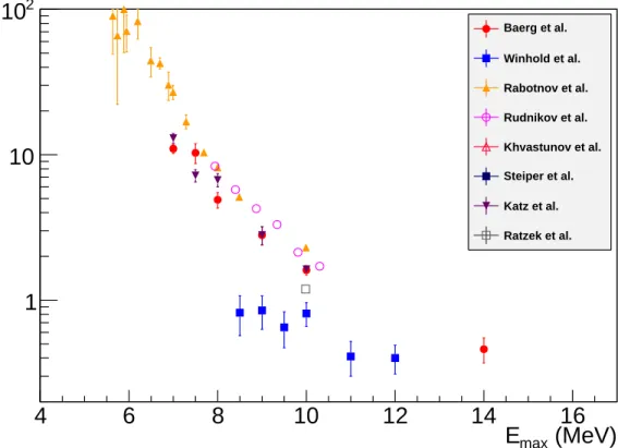
The b/a ratio of 238U is plotted as a function of endpoint energy, Emax, for all

previous bremsstrahlung measurements in Fig. 4.1. The data sets for232_{Th are included}

in Fig. 4.2. The general trend of decreasing b/a with photon energy is consistent for

(51)

(MeV)

max

E

5

6

7

8 9 10

20 b/a

-2

10

-1

10

1

10

2

10

Baerg et al. Winhold et al.

Soldatov et al. Rabotnov et al.

Rudnikov et al. Carvalho et al.

Khvastunov et al. Forkman et al.

Baz et al. Dowdy et al.*

Forkman et al.* Manfredini et al.*

Figure 4.1: The b/a ratios for the photofission of 238_{U have been plotted for all}

previ-ous measurements to date. There is a clear trend toward decreasing anisotropy with increased Emax. The data sets are taken from [24, 36, 39, 40, 42–45, 48]. The three

entries in the legend marked with an asterisk employed capture gamma rays whereas all other measurements used a bremsstrahlung photon beam. The monoenergetic data sets have been plotted such thatEmax =Eγ.

(52)

(MeV)

max

E

4

6

8

10

12

14

16 b/a

1

10

2

10

Baerg et al.

Winhold et al.

Rabotnov et al.

Rudnikov et al.

Khvastunov et al.

Steiper et al.

Katz et al.

Ratzek et al.

Figure 4.2: Theb/a ratios from232Th measured with bremsstrahlung beams. The data sets are taken from Refs. [24, 36, 39, 43, 48].

the averaged value of all contributing states lower in energy. The measurements using monoenergetic beams, on the other hand, probe only the states within the energy width of the gamma ray beam incident on the target.

Another clear result is that the anisotropy associated with232Th is much larger than that with238_{U, see Fig. 4.3. One perspective on the issue could be that it is the result}

of a difference in barrier structures. It is known that the inner barrier is higher than the outer barrier in238U whereas it is opposite in 232Th [52]. This difference has large implications to sub-barrier fission, as will be discussed in Sect. 4.5, and could potentially be the source of this above-barrier observation as well. Another applicable consideration

(53)

(MeV)

γ

E

5

6

7

8

9

10 b/a

1

10

2

10 232Th

238U

Figure 4.3: Theb/aratios for the photofission of238_{U and}232_{Th are plotted. The}232_Th

displays a significantly larger anisotropy than238U. Data are taken from Ref. [43]. provided by Schmitt and Duffield [53], is the absence of yields corresponding to mass-symmetric splits for232_{Th below 7 MeV; the same is not true of}238_{U. Symmetric fission}

(54)

4.3 Correlation of Angular Anisotropy and

Mass-Asymmetry

Since the discovery of PFADs, it has also been known that, in 232Th, the fragment mass asymmetry is correlated with the anisotropy. Using bremsstrahlung beams of

Emax= 16 MeV, a nearly-linear relationship was observed between the mass asymmetry

of the fragments, presented as the ratio of their masses, and the b/a quantity [36, 54]. In a more recent experiment, Steiper and coworkers [49] have observed the same general phenomenon using bremsstrahlung beams of Emax between 10 and 12 MeV.

Their results corroborate the fact that the anisotropy is increased for fission events characterized by greater mass asymmetry.

4.4 Quadrupole Photofission

Fission proceeding through Jπ _{= 2}+ _{states has gained much attention for energies}

at or below the fission barrier, 5 to 6 MeV, though many measurements up to 10 MeV have also been made. According to Bohr’s theory, this is expected to proceed through the first excited state of the even-parity, K = 0 rotation band, see Fig. 3.3. The reporting of “quadrupole” fission has concentrated on the ratio of the c parameter to the b parameter in Eq. 3.10. Thec parameter carries the most significant information because it is nonzero only if there are transition states ofJ = 2+ _{involved in the fission}

event. The converse is not true because thecterm is composed of the three quadrupole

(55)

channels, see Eq. 3.11, as

c= 15 16u−

5 4v+

5

16w. (4.3)

There are many combinations of these parameters that will cause c to be zero. The ratio of the cto b terms provides a little more information but still limited.

Knowing these facts, it is now possible to consider the results of previous experi-ments. At first glance, the data sets for238_{U are, with exception of the data of Baz}_{et al}_.

[37], coherent with one another, see Fig. 4.4. However, it is unclear whether the results of Ref. [42] and Ref. [43] are completely independent or are merely the reanalysis of the same data set. If the same data set has been used by both, then the data points below 6 MeV are the only measurements of that energy range. This would mean that the data sets are only in agreement whenEmax ≈6.5 MeV. At higher energies the results

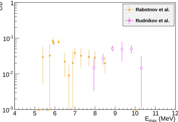
of separate measurements are in great disagreement so that little can be concluded. As regards 232_{Th, there are two data sets published that overlap slightly. Together}

these data sets indicate that thec/bratio does not change magnitude as significantly as theb/aratio does forEmax between 6 MeV and 10 MeV. However, within this range lots

of interesting energy dependencies exist. The large error bars make it difficult to assign great meaning to these fluctuations but they are statistically significant variations given the reported error bars.

(56)

so subsequently reduces the number of free parameters in the unpolarized angular distribution by one. There is some ambiguity in doing this however, because the c

parameter can be small or zero when contributions of 2+ transition states to the cross section are actually large, see Eq. 4.3. Regardless, there have been many conclusions formed with cfixed at zero.

(MeV)

max

E

4

6

8

10

12

14

16 c/b

-3

10

-2

10

-1

10

1

Soldatov et al.

Rabotnov et al.

Rudnikov et al.

Forkman et al.

Baz et al.

Figure 4.4: The c/b ratios from 238U(γ, f) measured using bremsstrahlung beams are plotted for all measurements to date. The data sets are taken from Refs. [37, 40, 42, 43, 48].

4.5 Barrier Systematics

The understanding of the potential energy surface has improved dramatically since the first experiments were carried out seventy years ago. The channel formalism of

(57)

(MeV)

max

E

4

5

6

7

8

9

10

11

12 c/b

-3

10

-2

10

-1

10

1

Rabotnov et al.

Rudnikov et al.

Figure 4.5: Thec/b values from232_{Th measured using bremsstrahlung beams are}

plot-ted for all measurements to date. The data sets are taken from Refs. [43, 48].

Bohr was created with the single-humped barrier predicted by the liquid drop model in mind. Today, it is believed that most of the actinides, including232_{Th and}238_{U, have a}

potential energy surface characterized by a triple-humped structure, see Fig. 2.3. Given the parameterization of the nuclear shape in Eq. 2.2, this corresponds to a quadrupole deformation with value β2 ≈ 0.9 and an octupole deformation of β3 ≈ 0.35 [18], see

(58)

and J = 1− states lead to structure in the energy dependence of the angular distribu-tion. Griffin was the first to consider the importance of this by considering the relative penetrations associated with each transition state [55]. The penetrationp(E) is equiv-alent to the probability for tunneling through a barrier and was estimated by Hill and Wheeler [56] to be

p(E) ={1 + exp [2π(Ef −E)/~ωf]}−1 (4.4)

for a barrier with the shape of an inverted parabola. The height of the fission barrier with respect to the ground state is given by Ef, ~ωf is a value indicative of the shape

of the barrier, and E is the excitation energy. If each transition state is considered to be a unique barrier, then this penetration factor is proportional to the probability for fissioning through specific transition states. Using this line of thinking, Griffin suggested that if the dipole fission barrier is greater than the height of the quadrupole barrier, as is consistent with the ideas of Bohr, then the energy difference between the barrier penetration would diminish the natural preference for E1 absorption considerably more than for E2. An increased importance of quadrupole fission would become pronounced in the angular distribution. The data of Refs. [42, 43] provide some evidence for this fact in238U because thec/bratio rises sharply as the energy decreases. Their interpretation began with the ideas of Griffin and concluded with a predicted energy dependence for the b/a and c/b ratios. It was stated in Ref. [43] that the interplay of the relative penetration through each of the barriers would cause both ratios to peak slightly below the point at which the energy dependence of the cross section is no longer determined

(59)

by the penetration factor. The 238_{U data alone do not support this beyond a doubt.}

However, the consideration of the 232_{Th data with the remaining collection of actinide}

data sets provides a more impressive body of corroborating evidence [35].

β

₂ E n er gy ( MeV ) GS 0 6

β

₂ E n er gy ( MeV

)

GS 0 6 a b

1-_,0

2+_,0 1

-_,0 2+_,0

Figure 4.6: A diagram of the different fission barrier heights assumed by Rabotnov et al. [43] and Vandenbosch [57] and generalized to a triple-humped barrier. A schematic triple-humped barrier is shown for the different energy (Jπ_{, K}_{) = (2}+_,_{0) and (1}−_,₀₎

transition states. The argument of Rabotnovet al. assumed the ordering of the states depicted in (a), which is in accord with Bohr’s hypothesis. Vandenbosch assumed that the the states became degenerate at the outermost barrier as shown in (b). Figure (a) also serves to illustrate his argument about the b/a ratio.

There has been little discussion of the effect of a triple-humped fission barrier on the angular distribution. On the other hand, much has been written with regard to the double-humped fission barrier. The arguments presented by Rabotnov et al.

(60)

data exhibit no significant rise in the c/bratio with decreasing energy.

A suitable explanation has been presented by Vandenbosch [57] and is based on three assumptions. They are that the inner barrier is lower than the outer barrier, the outer barrier corresponds to a reflection-asymmetric state, and the angular distribution is determined at the outermost barrier. According to recent calculations, see Fig. 2.3, the first two of these are well satisfied. The third assumption is well justified because a deep potential well separating the two barriers could destroy angular distribution because ofK-mixing [43]. A reflection-asymmetric nucleus has an excitation spectrum containing a 1− state comparable in energy to the 2+ state in the “ground-state” band, see Fig. 4.6. Because of this fact, greater inhibition of the dipole channel by barrier penetration is not present in232_{Th. The explanation of Vandenbosch also addresses the}

much smallerb/aratio for238U as compared to232Th. In238U, the outer barrier is lower than the inner barrier. The energy required to overcome the inner barrier will result in a greater excitation energy at the outer barrier. As such, enough energy will exist to excite nonzero K states, which will wash out the angular anisotropy. The situation is opposite in 232_{Th, because the outer barrier is highest. The nucleus will be colder}

at the point critical for determining the angular distribution so that only the lowest energy states will be able to contribute. Only K = 0 states will contribute, and the anisotropy will arise almost purely from theK = 0 state.

(61)

4.6 Prompt-fission neutrons

Recent efforts at TUNL that I have been involved with have led to first observations of anisotropies in prompt fission neutron angular distributions (NADs) [1]. Photofis-sion was induced in238U, 232Th, 235U, and 239Pu using 100% linearly-polarized photon beams with energies between 6 and 10 MeV. Neutrons were detected in the plane of polarization and perpendicular to it. The anisotropy with respect to rotations about the beam axis has been characterized by the asymmetry, Σ, which is defined as

Σ(θ) = Y(θ)k−Y(θ)⊥

Y(θ)k+Y(θ)⊥

. (4.5)

The quantity Y(θ)⊥ is the yield measured at angle θ. The subscript ⊥ indicates that

the detector was positioned at φ = 90◦ or φ = 270◦, whereas k indicates φ = 0◦ or

φ = 180◦. A few observations are worth making about these data. First is that the neutron asymmetries are nonzero for even-even nuclei whereas they are nearly zero for odd-A nuclei. The reason for this is believed to be related to the number of K states involved in the reaction. An even-even nucleus that absorbs a photon is only excited to a 1−, 2+_{, or 1}+ _{state with any noticeable probability. Because the odd-A nuclei}

(62)

Since the majority of prompt fission neutrons are evaporated from already accelerated fragments, this gives a reason to believe that the neutron asymmetry is largely the result of an underlying fission fragment asymmetry. As such, a complete understanding of the prompt neutron angular distributions would benefit from understanding the FAD produced with nearly-monoenergetic, 100% linearly-polarized photon beams. Since no measurements of this sort have been carried out in the past, this need will be addressed by the present thesis work.

(MeV)

γ

E

)

°

(90

_n

Σ

-0.2 0 0.2 0.4 0.6 0.8

5.6 6.2 6.8 7.4

exp exp exp exp

U

235

U

238

Pu

239

Th

232

Figure 4.7: The nonzero prompt fission neutron asymmetries measured using 100% linearly-polarized beams at HIγS [1]. The asymmetries, Σn, defined as Σn(θ) =

[Yn(θ, φ= 0)− Yn(θ, φ= 90◦)]/[Yn(θ, φ= 0) +Yn(θ, φ= 90◦)] whereYn is the neutron

yield.

(63)

Chapter 5 The Experiment

5.1 Description of the Experiment

Two distinct data collection efforts were conducted to measure polarized-photofission angular distributions. A measurement of this type requires a number of key compo-nents: a beam of incident polarized gamma rays, a target, charged-particle detection system, and data-readout system. The first of these was readily produced at Triangle Universities Nuclear Laboratory (TUNL) by the HIγS facility, which produces high-intensity and high-resolution photon beams with 100% polarization. The beams it produced were incident on either a 232_{Th or} nat_{U target where photofission was}

(64)

sys-tion 5.3, the relevant details of detector operasys-tion will be described in Secsys-tion 5.4, and the data-readout system will be explained in Section 5.5.

5.2 Experimental setup

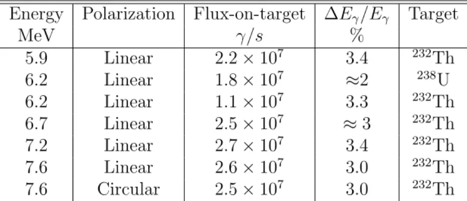
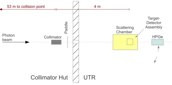
The HIγS facility produced nearly-monoenergetic photon beams by means of Comp-ton backscattering inside the optical cavity of a storage ring based free-electron laser (FEL). These had a pulsed temporal structure with frequency of 5.58 MHz that re-sulted directly from the periodicity of the electron bunches from which the FEL light backscattered. During this project, the beams were produced with energies between 5.7 and 7.6 MeV and fluxes-on-target between 1 x 107 γ/s and 2 x 107 γ/s, see Table 5.1. The HIγS facility is capable of producing either 100% linearly-polarized or circularly-polarized beams. Circularly-circularly-polarized beams were used to measure systematic differ-ences between detectors at the same polar angle that are attributable to geometry, strip functionality, and signal processing. Prior to reaching the target, the beams were collimated to a diameter of 1.91 cm using a Pb collimator. In order to monitor the flux while the beam was incident upon the target, two separate plastic scintillator sys-tems, one in each experimental effort, were used. The energies of these beams were measured using a high-purity germanium (HPGe) detector that was positioned in the beam during energy measurements, see Fig. 5.1.

The collimated photon beams passed through the center of an evacuated scattering chamber that contained the target and the detectors, see Fig. 5.2. The scattering

(65)

Energy Polarization Flux-on-target ∆Eγ/Eγ Target

MeV γ/s %

5.9 Linear 2.2×107 3.4 232Th 6.2 Linear 1.8×107 _≈₂ 238_U

6.2 Linear 1.1×107 _3.3 232_Th

6.7 Linear 2.5×107 ≈3 232Th 7.2 Linear 2.7×107 _3.4 232_Th

7.6 Linear 2.6×107 _3.0 232_Th

7.6 Circular 2.5×107 3.0 232Th

Table 5.1: The list of photon beam energies and characteristics to measure a particular target. No beam profiles were measured for the 6.7 MeV 232_{Th and 6.2 MeV} 238_U

data sets, so no measured energy spreads are included. However, in both cases, beam characteristics were measured for photons beams nearby in energy and collimated with the same collimator. Inferred values based on these representative measurements are included as approximate values.

ber pressure was maintained at approximately 10−5 _{Torr to ensure that the fragments}

were able to traverse the distance between the target and the detectors unhindered. Each target was rotated for the purpose of avoiding geometry-related detection bias between paired detectors. The rotation was defined by the set of Euler anglesφ = 42◦,

θ = 59◦, and ψ = 30◦. This rotation assumes that the surface normal of the target’s largest area side is oriented parallel to the positive z-axis defined by the downstream beam axis prior to rotation.

(66)

Photon beam

UTR

Scattering Chamber

HPGe

Collimator Hut

Collimator

P

a

d

le

Target-Detector Assembly

53 m to collision point 4 m

Figure 5.1: The layout of the experiment in the UTR. The photon beam is collimated first and then subsequently encounters the paddle system, the scattering chamber, and finally the HPGe detector. The HPGe detector was positioned out of the beam when not measuring the beam energy. The target and detector assembly reside inside the scattering chamber.

detect those at primarily less than 90◦. The target was positioned over the downstream pair of detectors so that fragments emitted at θ = 90◦ could be detected, which is the angle corresponding to the largest predicted asymmetries. The polarization dependent term of Eqs. 3.10 and 3.18 has a minimum at φ = 90◦ and φ = 270◦, whereas it peaks at φ = 0◦ and φ = 180◦. To be sensitive to this φ dependence, paired detectors were positioned differently in the φ direction by 90◦. One was positioned at either

φ= 0◦,180◦ and the other was atφ = 270◦,90◦, respectively. In this way, a single pair of detectors was sensitive to the extreme values of the polarization dependent term of the angular distribution.

The detector-target assembly was designed to minimize shadowing effects. Shadow-ing is the inhibition of a fragment from beShadow-ing detected due to the presence of material