THERMODYNAMICS OF ONE-DIMENSIONAL MANY-FLAVOR FERMIONS AT FINITE TEMPERATURE: DENSITY, PRESSURE, COMPRESSIBILITY, AND
CONTACT
Michael Hoffman
A dissertation submitted to the faculty at the University of North Carolina at Chapel Hill in partial fulfillment of the requirements for the degree of Doctor of Philosophy in the
Department of Physics.
Chapel Hill 2017
ABSTRACT
Michael Hoffman: Thermodynamics of one-dimensional many-flavor fermions at finite temperature: density, pressure, compressibility, and contact
(Under the direction of Joaquin Drut)
Motivated by advances in the manipulation and detection of ultracold atoms with mul-tiple internal degrees of freedom, we present a finite-temperature lattice Monte Carlo calcu-lation of the density and pressure equations of state, as well as Tan’s contact, of attractively interacting SU(2)-, SU(4)-, and SU(6)-symmetric fermion systems in one spatial dimension. We also furnish a nonperturbative proof of a universal relation whereby quantities com-putable in the SU(2) case completely determine the virial coefficients of the SU(Nf) case.
To my wife and son: for the inspiration, support, and happiness you have given me
ACKNOWLEDGEMENTS
I have had the good fortune while completing this work to have been supported by many great people. I would like to begin by thanking my parents for setting me upon the path of learning and scholarship.
I would like to thank my wife’s parents for their support while both Marta and I were pursuing our degrees. Especially, Helena, for coming to live with us and watch over our son during the first two years of his life. Without your help, it would not have been possible to stay sane and productive while doing research and learning to be parents.
My wife, Marta, deserves a special thanks. There were many long nights I shared with you working together on our own projects. I look forward to many more to come.
I have benefited from my collaborators Jay Porter, Andrew Loheac, Eric Anderson for many interesting discussions, criticisms, and fun over the course of this work. Thank you all.
TABLE OF CONTENTS
LIST OF TABLES . . . ix
LIST OF FIGURES . . . x
LIST OF ABBREVIATIONS AND SYMBOLS . . . xiii
1 Introduction to one-dimensional fermions . . . 1
1.1 Introduction . . . 1
1.2 Basic Statistical Mechanics of Bosons and Fermions . . . 1
1.2.1 The partition function . . . 2
1.2.2 Ideal Bose gas . . . 3
1.2.3 Ideal Fermi gas . . . 5
1.2.4 Overview of Fermi liquid theory . . . 6
1.3 One dimensional interacting Fermi gases . . . 8
1.3.1 Luttinger liquids . . . 8
1.3.2 Bosonization . . . 14
1.4 Overview of experimental results . . . 17
1.5 Quantum many-body problem on the lattice . . . 20
1.5.1 Defining the problem on the lattice . . . 20
1.5.2 Path integral formulation . . . 20
REFERENCES . . . 27
2 Universality in one-dimensional two-flavor fermions at finite tempera-ture: Density, pressure, compressibility, and contact . . . 31
2.1 Introduction . . . 31
2.2 Many-body method, scales and dimensionless parameters . . . 33
2.3 Results . . . 34
2.3.1 Density . . . 35
2.3.2 Temperature scale . . . 37
2.3.3 Pressure and compressibility . . . 38
2.3.4 Contact . . . 41
2.4 Summary and Conclusions . . . 43
2.5 Systematics of the approach to the continuum limit . . . 44
REFERENCES . . . 47
3 Thermodynamics of one-dimensional SU(4) and SU(6) fermions with attractive interactions. . . 50
3.1 Introduction . . . 50
3.2 Many-body method, scales and dimensionless parameters . . . 52
3.3 Results . . . 54
3.3.1 Density . . . 55
3.3.2 Pressure and compressibility . . . 57
3.3.3 Tan’s contact . . . 58
3.3.5 Empirical Fitting . . . 68
3.4 Summary and Conclusions . . . 70
3.5 Systematics of the approach to the continuum limit . . . 73
3.6 Derivation of partition function formula for Nf flavors . . . 73
REFERENCES . . . 78
4 Conclusions and Future Work. . . 83
4.1 Conclusions . . . 83
LIST OF TABLES
1.1 Bosonization Dictionary: An overview of the key features results of the bosoniza-tion formalism. The notabosoniza-tion is a combinabosoniza-tion of expressions from Giamarchi [21] and von Delft [15]. . . 15 2.1 Fit parameters for the density equation of state, using the functional form
n/n0 = 1 +α(βµ)−γ, second-order pressure virial coefficient b
2, and
LIST OF FIGURES
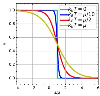
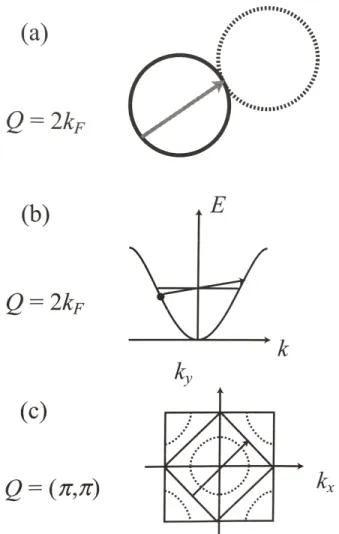
1.1 Occupation number for the ideal Fermi gas at various temperatures. The step function (light blue) is forT = 0. . . 6 1.2 The nesting properties of Fermi surfaces for high dimensions (a) and one
dimension (b). A small subset of points are nested for Q = 2kF in high
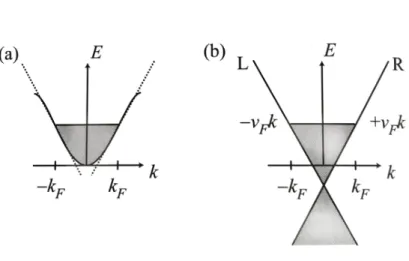
dimensions compared to the perfectly nested pair of points in one dimension. In (c) we see that it is possible to construct highly nested Fermi surfaces in higher dimensions, in this case, a square Fermi surface in two dimensions. Reproduced from [15]. . . 10 1.3 Typical quadratic dispersion relation (a) is simplified to a linear spectrum (b).
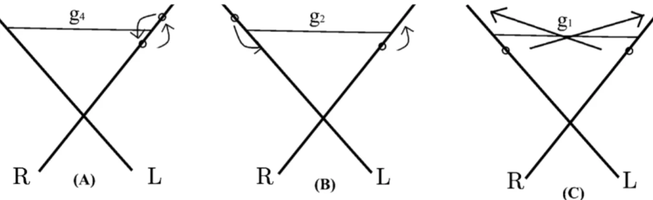
Adapted from [15]. . . 11 1.4 The low energy interaction processes are summarized into three sectors.
Pro-cess g4 (A) couples only fermions on the same branch above and below the
Fermi point. Process g2 (B) couples fermions from one branch to the other
without exchange. Processg1 (C) corresponds to coupling fermions on
oppo-site branched with exchange. . . 12 1.5 Experimental confinement of two-component ultracold 6Li atoms trapped in
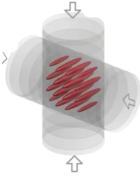
an array of 1D tubes. The grey lines represent the laser beams used to make the traps. The arrows represent the direction the beams are propagating. In total, four counter-propagating laser beams interfere to form a standing wave (peaks and trough represented by shading). In typical setups trapping frequencies along the tube axis are between 10-200 Hz while radial frequencies are as high as 100 kHz. From Blocket al. [34]. . . 18 1.6 A 2D optical lattice is used to create an array of independent quantum wires
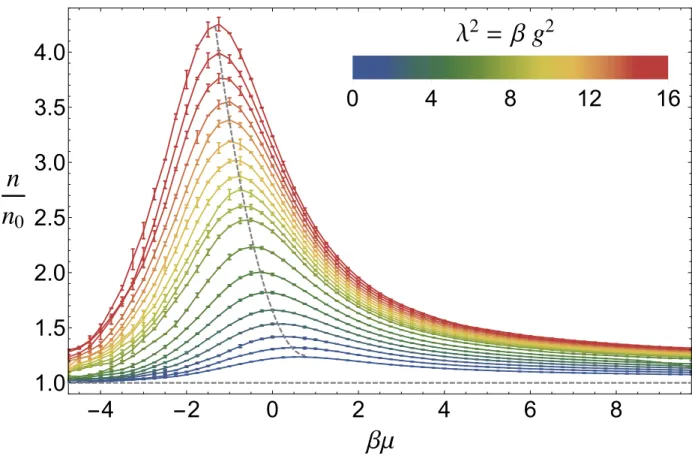
of ultracold 173Yb (the spheres) with six possible nuclear spin orientations (arrows and colors). The important distinction to make in this graphic is the many spins confined to each tube. From Paganoet al. [38]. . . 19 2.1 (Color online) Densityn, in units of the density of the non-interacting system
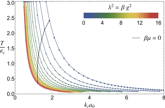
n0, as a function of the dimensionless parametersβµ= lnzandλ2=βg2. From bottom to top, the coupling isλ= 0.0,1.0,1.25,1.5, ...,2.5,2.75,3.0,3.1,3.2, ...,4.0. The dashed line joins the maxima at eachλ. . . 35 2.2 (Color online) Temperature scale, in units ofεF, as a function of the coupling
kFa0. Here, kF = πn/2, where n is the total density, and εF = k2
F/2. The
dashed line connects theβµ= 0 points for each value of λ. Theβµ >0 (<0) points lie to the right (left) of the dashed line. . . 38 2.3 (Color online) Pressure in units of its non-interacting counterpart, as a
func-tion of the dimensionless parameters βµ = lnz and λ2 = βg2, obtained by
2.4 (Color online) Isothermal compressibility in units of its non-interacting coun-terpart, as a function of the dimensionless parametersβµ= lnz andλ2 =βg2.
The values of λ shown in this plot are the same as in Fig. 2.1, but from top to bottom instead. . . 40 2.5 (Color online) Tan’s contact C, scaled by βλT/(2Q1λ2) = πβ2/(2Lλ2) [see
Eqs. (2.13) and (2.14)], as a function of βµ. The black line shows C in the absence of interactions. Inset: Zoom-in of main plot on the region −4.5 ≤ βµ≤ −1.0, showing also the leading-order virial expansion. Both plots show data for λ= 0.5,1.0,1.5, ...,4.0, which appear from bottom to top. . . 42 2.6 (Color online) Density n, in units of the non-interacting density n0, as a
function of βµ at weak coupling (λ = 1.0), for several values of β. Finite-β effects are small throughout the graph. Note the ranges in the x and y axes are different from those of Fig. 2.1. . . 45 2.7 (Color online) Densityn, in units of the non-interacting densityn0, as a
func-tion ofβµ at the strongest coupling in this study (λ= 4.0), for several values ofβ. Finite-βeffects are clearly visible, especially around the maximum. Note that thex-axis range is different from that of Fig. 2.1, but they-axis is slightly extended. . . 46 3.1 (Color online) Density n for Nf = 4, in units of the density of the
non-interacting systemn0, as a function of the dimensionless parametersβµ= lnz andλ2=βg2. From bottom to top, the coupling isλ= 1.75,2.0,2.25,2.5,2.75,3.0.
The data points come from the QMC calculations and the solid lines are from the fits (see Eq. 3.32). . . 56 3.2 (Color online) Density n for Nf = 6, in units of the density of the
non-interacting systemn0, as a function of the dimensionless parametersβµ= lnz andλ2=βg2. From bottom to top, the coupling isλ= 1.75,2.0,2.25,2.5,2.75,3.0.
The data points come from the QMC calculations and the solid lines are from the fits (see Eq. 3.32). . . 57 3.3 (Color online) Pressure forNf = 4 in units of its non-interacting counterpart,
as a function of the dimensionless parameters βµ = lnz and λ2 = βg2, ob-tained by βµ-integration of the density (see Eq. 3.7). The values ofλ shown in this plot are the same as in Fig. 3.1. . . 59 3.4 (Color online) Pressure forNf = 6 in units of its non-interacting counterpart,
as a function of the dimensionless parameters βµ = lnz and λ2 = βg2,
ob-tained by βµ-integration of the density (see Eq. 3.7). The values ofλ shown in this plot are the same as in Fig. 3.1. . . 60 3.5 (Color online) Isothermal compressibility for Nf = 4 (top) and Nf = 6
(bot-tom) in units of its non-interacting counterpart, as a function of the dimen-sionless parametersβµ = lnz and λ2 =βg2. The values of λ range from 0 to
3.6 (Color online) Isothermal compressibility for Nf = 6 in units of its
non-interacting counterpart, as a function of the dimensionless parameters βµ = lnz and λ2 =βg2. The values of λ range from 0 to 3.0 in steps of 0.125. . . . 62 3.7 (Color online) Tan’s contactC forNf = 4, scaled byβλT/(2Q1λ2) =πβ2/(2BNfLλ2),
as in Ref. [29], as a function of βµ, for λ= 1.75,2.0,2.25,2.5,2.75,3.0, which appear from bottom to top. The value BNF is the binomial coefficient Nf
choose 2; this scale factor was chosen to facilitate comparison between flavors. 63 3.8 (Color online) Tan’s contactC forNf = 6 (bottom), scaled byβλT/(2Q1λ2) =
πβ2/(2B
NfLλ2), as in Ref. [29], as a function ofβµ, forλ= 1.75,2.0,2.25,2.5,2.75,3.0,
which appear from bottom to top. The value BNF is the binomial coefficient
Nf choose 2; this scale factor was chosen to facilitate comparison between
flavors. . . 64 3.9 (Color online) Scaling fit parameter b of Eq. (3.32) as a functions of the
in-teraction strengthλforNf = 2,4,6. The data points are the results obtained
by fitting the Monte Carlo data; the solid lines are the fits to this data. . . . 70 3.10 (Color online) Amplitude fit parameterAof Eq. (3.32) as a functions of the
in-teraction strengthλforNf = 2,4,6. The data points are the results obtained
by fitting the Monte Carlo data; the solid lines are the fits to this data. . . . 71 3.11 (Color online) Shift fit parameter ξof Eq. (3.32) as a functions of the
interac-tion strength λ for Nf = 2,4,6. The data points are the results obtained by
fitting the Monte Carlo data; the solid lines are the fits to this data. . . 72 3.12 (Color online) Density n for Nf = 4, in units of the non-interacting density
n0, as a function of βµ at weak coupling (λ = 1.0), for several values of β. Finite-β effects are clearly minimal, even around the maximum. Note the ranges in thexand yaxes are different from those of Fig. 3.1 in order to focus on the regions with the most systematic effects more thoroughly. . . 74 3.13 (Color online) Density n for Nf = 4, in units of the non-interacting density
n0, as a function of βµ at the strongest coupling in this study (λ = 3.0), for several values of β. Finite-β effects are clearly visible, around the maximum. Note the ranges in the x and y axes are different from those of Fig. 3.1. . . . 75 3.14 (Color online) Density n for Nf = 6, in units of the non-interacting density
n0, as a function of βµ at weak coupling (λ = 1.0), for several values of β. Finite-β effects are minimal even around the maximum. Note the ranges in the x and y axes are different from those of Fig. 3.2. . . 76 3.15 (Color online) DensitynforNf = 6, in units of the non-interacting densityn0,
LIST OF ABBREVIATIONS AND SYMBOLS
Z Grand-canonical partition function
Q1 Single-particle partition functions
β Inverse temperature
µ Chemical potential
V Volume
T Temperature
n Density
n0 Density of free gas
P Pressure
κ Isothermal compressiblity
C Tan’s contact
~ Reduced Planck’s constant kB Boltzman’s constant
m fermion mass
L Length of system in lattice units
z Fugacity
g Coupling strength
a0 Scattering length
λ Thermal wavelength
Nx Number of lattice sites in thex direction
Nτ Number of lattice sites in the imaginary time direction
Nf Number of flavors
F Fermi energy
kF Fermi momentum/wavenumber
ˆ
H Hamiltonian operator ˆ
T Kinetic energy operator ˆ
V Potential energy operator
a†k,s(ak,s) Fermion creation (annihilation) operator
b†k,s(bk,s) Fermion creation (annihilation) operator
ψ(x), ψF(x) Fermion field
φ(x), ψB(x) Boson field
ˆ
n, ρ Density operator
u, K Luttinger liquid parameters
tr ,Tr Trace
det Determinant
σ Auxillary field
Lis Polylogarithm function of order s
HS Hubbard-Stratonovich
MC Monte Carlo
HMC Hybrid Monte Carlo
CHAPTER 1: Introduction to one-dimensional fermions
Section 1.1: Introduction
Everything in the physical world consists entirely of interacting quantum many-body sys-tems. Therefore, it is not surprising that these systems have been the focus of a tremendous amount of research. The majority of that work has made use of the powerful method of perturbation theory adapted to quantum field theory by Feynman [1] in 1949. The work in this dissertation will apply to strongly coupled systems that invalidate the assumptions of perturbation theory; and, therefore, require solution by numerical techniques. The purpose of this introductory chapter is to touch on a small subset of topics necessary to understand those techniques and topics introduced in the remaining chapters.
Section 1.2: Basic Statistical Mechanics of Bosons and Fermions
A long-standing goal of physics has been to understand the macroscopic physical prop-erties, thermodynamics, of a material by the specification of its microscopic behavior which is often much simpler. In classical mechanics, it is possible to have complete knowledge of a system if the position and momentum of each individual particle is specified at one par-ticular moment in time. Given the incredibly large number of particles contained in even a modest amount of material this requirement is not practical for calculations. In order to make progress a formalism for discarding irrelevant information to obtain a useful average quantity must be developed. That formalism is statistical mechanics [2, 3, 4].
all the known particles into two distinct classes: bosons and fermions [8]. Bosons are par-ticles where it is possible to put many of them in the same quantum state while fermions, by virtue of the Pauli exclusion principle, can have a maximum of one particle per quantum state. After these revelations, the foundation of ensemble theory was rebuilt and generalized into the familiar forms we see today as recounted by Flamm [9]. The remainder of the chap-ter will highlight the important features of these topics in relation to inchap-teracting many-body quantum systems with an emphasis placed on systems comprised of fermions.
1.2.1: The partition function
The partition function is the name given to the mathematical quantity that holds all the information necessary to extract statistical information from a physical system. This is the fundamental object in statistical mechanics because it determines how the microscopic details of the system conspire to produce the macroscopic thermodynamics of the system. This function in a particular formulation, called the grand-canonical partition function, for a system in equilibrium with Hamiltonian ˆH, inverse temperature β = 1/kBT, chemical
potential µ, and volume V can be written as:
Z(β, µ, V) = tr e−β( ˆH−µNˆ)=e−βΩ(T ,µ,V) (1.1)
where ˆN is the particle number operator, Ω is the grand canonical potential or thermody-namic potential, and the trace, tr , is to be performed over the Fock space comprised of all possible multi-particle states. In all the systems studied in this work the Hamiltonian will take the form:
ˆ
H = ˆT + ˆV (1.2)
the potential energy term will incorporate the information about the interaction and be di-agonal in coordinate space representation. An important difference between the operators is that the kinetic energy is a one-body operator: each term, in a summation over the discrete particles of the system, only requires information from one particle. The potential on the other hand is a two-body operator: each term in the expression requires information from a pair of particles -typically the distance between them. For a system of non-relativistic spin 1/2 fermions of mass m the kinetic energy is given by
ˆ T =X
k,s
~2k2 2m a
†
k,sak,s =
Z d3p
(2π)3
p2
2m(ˆn↑(p) + ˆn↓(p)) (1.3)
where a†k,s(ak,s) is the fermion creation (annihilation) operator for wavenumber k and spin s; and ˆns(p) is the density operator for particles of spins and momentum p. In the discrete
case the momentum can only take values given by p =~k = ~2πn/L where n is an integer and L is the size of the system. Throughout this dissertation, the potential energy will be given by a contact interaction parameterized by the bare coupling constant g, such that
ˆ
V =−gX
i
ˆ
n↑(x)ˆn↓(x) =−g
Z
d3xnˆ↑(x)ˆn↓(x) (1.4)
where ˆns(x) is the density operator for particles of spin sat positionx. It is from this
frame-work we will build the interacting systems; however, we will often compare the interacting systems governed by the Hamiltonians above to the free boson or free fermion systems at similar macroscopic parameter. Therefore, a short review is in order.
1.2.2: Ideal Bose gas
In a system of non-interacting bosons, the grand canonical partition function can be expressed as:
Z(β, µ, V) = ∞
X
N=0 N X
{nk}
e−βPk(εk−µ)nk =Y k
1
whereN is the total number of fermions,nkis the number of fermions in single particle state
k (often called the occupation number), and{nk}represents a particular way of distributing
the N particles among the single particle states. It is often convenient to work with the thermodynamic potential, Ω, which we can obtain my taking the natural logarithm of the partition function
Ω = P V kBT
=−kT X
k
ln(1−e−β(εk−µ)) (1.6)
This formulation of the partition function leads to a divergence when εk = µ. This can
be seen more clearly if we look at the number of particles in the system
N =X
k
nk = X
k
1
eβ(εk−µ)−1 (1.7)
where each value ofnkis positive and thereforeµ≤εk. For a non-relativistic particleεk≥0,
implies µ ≤ 0. Another way of viewing this restriction is to look at the density of states. The non-relativistic density of states for a gas in three dimensions is given by
a(ε)dε= 2πV h3 (2m)
3/2ε1/2 (1.8)
From this we can immediately obtain the thermodynamic potential
Ω = −2πV h3 (2m)
3/2 Z ∞
0
ε1/2ln(1−e−β(ε−µ))dε (1.9)
where the last term comes from treating theε= 0 term in the sum by itself. As the quantity βµ → 0 the fugacity z ≡ eβµ approaches unity and the term corresponding to the ground
1.2.3: Ideal Fermi gas
The partition function for fermions can be derived by starting with Eq. (1.5) and applying the further restriction that nk= 0,1. Thus
Z(β, µ, V) = ∞
X
N=0 1 X
nk=0
e−βPk(εk−µ)nk =Y k
(1 +e−β(εk−µ)) (1.10)
This restriction is a direct consequence of the Pauli exclusion principle rooted in the spin-statistics theorem [8]. Fermions are defined by their unwillingness to be in the same state; however, they are still orderly as the temperature of the system is lowered. Each fermion will want to find the lowest available state to occupy
nk=
1
eβ(k−µ)+ 1 (1.11)
as T → 0, this distribution becomes a step function where all the states up to the Fermi energy, F, are occupied, and all the states above are empty as shown in Fig. 1.1. This
orderly behavior gives rise to the patterns in the periodic table of elements and many other interesting low-temperature quantum phenomena as well.
The point in Fig. 1.1 where /µ = 1.0 is the Fermi energy. The energy for a non-relativistic fermion on that line is then F = ~
2k2
F
2m . Where the Fermi wavevector (Fermi
momentum in natural units) is kF = (6π2n/Nf) 1/3
in three dimensions with n = N/V and Nf is the number of flavors. In two dimensions kF = (4πn/Nf)1/2 and in one dimension
kF =nπ/Nf where the volume,V, changes appropriately for each dimension. The wavevector
sets the energy scale for the lowest level excitations of the system. To see why, I again refer back to Fig. 1.1 where even at finite temperature the states belowkF are highly occupied and,
4
2
0
2
4
6
/
0.0
0.2
0.4
0.6
0.8
1.0
n
4
2
0
2
4
6
/
0.0
0.2
0.4
0.6
0.8
1.0
n
kBT = 0
kBT = /10
kBT = /2
kBT =
Figure 1.1: Occupation number for the ideal Fermi gas at various temperatures. The step function (light blue) is forT = 0.
surface at zero temperature will be the surface of a sphere centered on the origin with radius kF, in two dimensions a circle, and in one dimension just the two points±kF from the single
k-axis.
1.2.4: Overview of Fermi liquid theory
used, such that: ~=m= 1.
The basis of the Fermi liquid theory is rooted in Fig. 1.1. For the T = 0 line, the magnitude of the discontinuity of the occupation number is unity. Excited states are created by adding particles to the system with a well-defined momentum k. These excitations have an infinite lifetime because they are eigenstates of the Hamiltonian. The spectral function, the probability of finding a state with momentumkand frequencyω, isA(k, ω) =δ(ω−ξ(k)), whereξ(k) = (k)−µis the energy with respect to the chemical potential. When interactions are switched on, Fermi liquid theory dictates that things should not really change that much. This is accomplished by redefining the essentially free particle in the system. The excitations in the system are no longer individual electrons, but electrons that are dressed by their interactions with the other electrons around them. The electrons are surrounded by particle-hole excitations of the ground state. The electron plus the density fluctuations of the particle-hole interactions are referred to as a quasiparticle. It is these quasiparticles that are essentially free.
The mass of a quasiparticles is not the mass of an electron, but a new rescaled mass that depends on the interactions of the system. A quasiparticle is not completely free so the spectral function is also modified, instead of a delta function one obtains a Lorentzian of width 1/τ where τ is the lifetime of the excitation. As discussed at the end of section 1.2.3, these excitations will likely take place near the Fermi surface. Therefore, we are permitted to replace the dispersion relation of the excitations with a linearized dispersion relation
E(k)'E(kF) +
kF
m∗(k−kF) (1.12)
avoiding perturbation theory. It should be noted, that the description above is a very brief overview that ignores residual interactions between quasiparticles and other features of Fermi liquids. However, this is all that is needed to show why the prevailing model of interacting fermions will break down in one dimension.
Section 1.3: One dimensional interacting Fermi gases
The remainder of the dissertation will focus on one dimensional systems. In short, the physics of one dimensional systems are drastically different than the ordinary three dimen-sional physics. In a basic sense the quantum fluctuations in these systems are more dramatic compared to their higher dimensional counterparts. This in itself is one reason to study the problem thoroughly [15]. From a purely theoretical point of view, they are unique because exactly solvable models exist for some one dimensional interacting problems, allowing for solutions in this space to serve as a starting point for more complicated problems and the development of an intuition for interacting quantum systems. From a numerical perspective, one dimensional problems have the smallest space-time volumes and can thus be studied to high accuracy with, relatively speaking, shorter computational time. This allows one dimen-sional systems to serve as benchmark for the development of new computational techniques. And finally, as the control of laboratory systems becomes ever more refined these systems have and will be realized experimentally and likely find use in applications in a variety of nano-devices.
1.3.1: Luttinger liquids
will be able to move freely. Individual excitations are essentially completely suppressed; therefore, only collective motion is allowed. This collective motion of all the fermions in the system invalidates the quasiparticle concept and thus Fermi liquid theory. This is the underlying reason one dimensional systems are theoretically interesting -a new method must be developed. The fundamental collective excitations in one dimensional systems are those of charge, like sound waves, and those of spin, like spin waves. In general, these excitations will have different group velocities and it is as if the electron has to break apart into two different fundamental excitations.
To develop a deeper understanding of why one dimensional systems are different than high dimensional systems we can look at the correlation functions of the system. For example, the susceptibility that measures the response of the system to an external potential is given by [16, 17]
χ(q, ω) = 1 V
X
k
fF(ξk)−fF(ξk+q)
ω+ξk−ξk+q+iδ
(1.13)
where V is the volume of the system, δ approaches zero from above, and fF is the Fermi
factor
fF(ξ) =
1
eβξ + 1 (1.14)
If we consider the static susceptibility, ω → 0, there is a divergence for any wavevector, Q, where ξk and ξk+Q are both zero. In high dimensions this can only occur for a small
Figure 1.2: The nesting properties of Fermi surfaces for high dimensions (a) and one dimen-sion (b). A small subset of points are nested for Q = 2kF in high dimensions compared
to the perfectly nested pair of points in one dimension. In (c) we see that it is possible to construct highly nested Fermi surfaces in higher dimensions, in this case, a square Fermi surface in two dimensions. Reproduced from [15].
indication that the ground state of the interacting system is quite different from the ground state of the free system. In order to solve the problem in the fermion framework we notice that due to the inversion property the Fermi velocity must be the same at±kF. This means
that near the Fermi surface it is possible to linearize the dispersion relation
ξ(k)'vF(k−kF) at k ≈kF (1.15)
which makes it clear that Q= 2kF satisfies the nesting condition.
This linear dispersion relation, see Fig. 1.3, leads to a Dirac sea of negative energies and to two species of fermions with one moving to the left and one moving to the right. The
Figure 1.3: Typical quadratic dispersion relation (a) is simplified to a linear spectrum (b). Adapted from [15].
Hamiltonian is now the Tomonaga-Luttinger Hamiltonian [18]
H = X
k;r=R,L
=vF(rk−kF)c
†
r,kcr,k (1.17)
where r in a subscript can take the value of R(L) for a right (left) moving fermion. If r is in an equation it will take the value r = 1 for a right moving fermion and r =−1 for a left moving fermion. To avoid infinities from infinite negative energy states we can choose an arbitrary momentum cutoff such that the energy is bounded around the fermi momentum kF ±Λ. In the fermion language, the single particle fermion operator becomes
ψ(x) = 1 V
X
k
eikxck '
1 V
X
k≈−kF
eikxck+ X
k≈kF
eikxck !
The fermion density operator is then
ρ(x)ψ†ψ(x) =ψ†L(x)ψL+ψ†R(x)ψR+ψL†(x)ψR+ψR†(x)ψL (1.19)
Figure 1.4 depicts the low energy processes we are interested in and they must be close to the Fermi points. The first two terms correspond to producing a particle-hole excitation on the same branch when q ≈0; and, the last two terms correspond to transporting a particle from one branch to the other when q ≈ 2kF. A branch refers to contour integration of the
propagators or more directly the types of fermions that can be produced in the system. In one dimension, this takes the form of right and left moving fermions which are produced on the right or left moving branches of the Fermi surface. It is then possible to rewrite the interaction as
Hint =
1 2V
X
k,k0,q
V(q)c†k+qc†k0−qck0ck (1.20)
The interactions can be summarized in three sectors or g-process (the analysis of which is referred to a g-ology.) These processes are illustrated in Fig. 1.4. The g4 process couples
Figure 1.4: The low energy interaction processes are summarized into three sectors. Process g4 (A) couples only fermions on the same branch above and below the Fermi point. Process
g2 (B) couples fermions from one branch to the other without exchange. Process g1 (C)
corresponds to coupling fermions on opposite branched with exchange.
to a left (right) moving fermion, but both remain on the same branch after the interaction. Lastly, the g1 process, backscattering, couples fermions where they exchange sides. Below I
will outline a solution of this problem first solved by Dzyaloshiniskii and Larkin in 1974 [19]. This solution is done in the fermion language and will highlight the difficulties with such an approach. This was the first solution of the problem and is considered a theoretical tour de force to this day.
The first complication that is encountered is the g1 process. The g1 process breaks the
solution; and, is therefore, ignored. This means we will discuss only spinless fermions where the g2 and g1 process are identical. Essentially, this simplification means the chirality of the
particle cannot be changed by the interactions. This reduces the problem to only diagrams with fermion bubbles with at most two interaction lines. All other terms will cancel. The symmetries that produce this cancelation are the linear dispersion relation and the inability to change chirality and is equivalent to the random phase approximation (RPA) [20]. The effective interaction equations in this case are thus
Γ4 =g4−g4ΠRΓ4−g2ΠLΓ2 (1.21)
Γ2 =g2−g4ΠRΓ4−g2ΠLΓ2 (1.22)
where ΠR,L are the bubbles of the right or left moving fermions cutoff at order two
ΠR=
−k 2π(iν−vFk)
(1.23) ΠL =
k 2π(iν+vFk)
(1.24)
If we set g4 = 0 the solution is simple to obtain and the effective interaction becomes
Γ2 =
g2
1−g2 2ΠRΠL
(1.25)
= g2(ν
2+v2 Fk2)
(ν2+v2
Fk2)−( g2
2πvF) 2(v
Fk)2
The poles in this solution suggest a new natural velocity of the system
u2 =v2F 1−
g2
2πvF 2!
(1.27)
This would mean the poles occur when iν =±uk. This solution shows that the excitations produced by the interactions have a well-defined energy-momentum relationship; in addition, the velocity of the excitations is renormalized by the interaction. Additional features of the theory are incredibly difficult and technical in the fermion language [15]. The purpose of this section was to highlight those difficulties and give a taste of the results. A more elegant solution is provided by the method of bosonization [21]. It is important to point out that while the conclusions drawn from the fermion language are the same as those to follow, they are much easier to arrive at in the bosonization language and thus the method is considered the natural language of the problem even for fermions.
1.3.2: Bosonization
The main theoretical tool for solving problems in one dimensional quantum systems is the method of bosonization. There are two main approaches to this topic: field theoretical [15] and constructive [21]. We will follow the approach of Giamarchi to make connections with the concepts in field theory; however, the constructive approach is more amenable to interpretation and refermionization.
In bosonization the interacting fermions are transformed into a system of massless, non-interacting bosons. The method dates back to 1975 when in the particle physics community Sidney Coleman and Stanley Mandelstam [22, 23] discovered the method at the same time of Daniel Mattis and Alan Luther [24, 25] in the condensed matter community. However, the theory was put in its modern form by Haldane in 1981 [26].
dimension [27].
The concepts in bosonization are often summarized in a bosonization dictionary as in Table 1.1. From the ingredients in the table you can see the flavor of the theory. Particularly, some of the details that will not be covered in this overview.
Table 1.1: Bosonization Dictionary: An overview of the key features results of the bosoniza-tion formalism. The notabosoniza-tion is a combinabosoniza-tion of expressions from Giamarchi [21] and von Delft [15].
Feature Notation of the expression
fermion operators {ck,η, c†k0,η0}=δkk0δηη0 where η = 1, . . . , Nf and k ∈[−∞,∞]
k-quantization 2πL(nk− 12δb), δb ∈[0,2), nk ∈Z
vacuum state ck,η|~0i0 ≡0 for k >0, , c
†
k,η|~0i0 ≡0 for k ≤0,
number operator Nˆη ≡ P
k:c
†
k,ηck,η := P
k h
c†k,ηck,η−0h~0|c
†
k,ηck,η|~0i0 i
boson creator b†qη = √i nq
P kc
†
k+q,ηck,η, q= 2πLnq, nq ∈Z +
boson commutator [bqη, b†q0η0] =δηη0δqq0
fixed N~ state Nˆη|N~i0 =Nη|N~i0, bqη|N~i0 = 0
Klein factor Fη†f(b†)|N~i0 ≡f(b†)c
†
Nη+1|
~ Ni0
F commutator [F, b] = 0, {F†
eta, Fη0}= 2δηη0, [ ˆNη, Fη0] =−δηη0Fη
fermion field ψη(x)≡ 2πL
1/2P ke
−ikxc kη
ψη commutator {ψη(x), ψ†η(x
0)}=δ
ηη02πδ(x−x0), |x−x0|< L
boson field φη(x)≡ −Pq>0 √1nq(e−iqxbqη+eiqxb†qη)e
−aq/2
φη, ∂xφη commutator [φη(x), ∂x0φη0(x0)] =δηη02πi(δ(x−x0)− 1
L)
bosonization ψη(x) =Fηa−1/2e−i
2π L( ˆNη−
1
2δb)xe−iφη(x)
(2π) density ρη(x) =:ψη†(x)ψeta(x) :=∂xφη(x) + 2πLNˆη
fermion Hamiltonian H0η ≡Pkk :c†kηck0η0 :=
RL/2
−L/2 dx 2π 1 2 :ψ
†
η(x)i∂xψη(x) :
bosonized Hamiltonian H0η = P
q>0qb
†
qηbqη+ 2πL 1
2Nˆη( ˆNη + 1−δb)
=R−L/2L/2 dx2π12 : (∂xφη(x))2 : +2πL 12Nˆη( ˆNη+ 1−δb)
The theory was developed by Haldane in 1981 [26] by first creating a labeling field φl(x)
to represent the location of all the particles. The field is continuous and increments in value by 2π between each particle; therefore, the value of the particle at position i is given by φl(xi) = 2πi. This means the field is an alternative way to number the particles. In one
density operator
ρ(x) = X
x
δ(x−xi) = X
n
|∂xφl(x)|δ(φl(x)−2πn) (1.28)
Now the field can always be taken to be increasing by starting the labeling at x = −∞ so the absolute value sign is no longer required and by applying Poisson summation can be rewritten in the more useful form
ρ(x) = ∂xφl(x) 2π
X
p
eipφl(x) →
ρ0 −
1
π∂xφ(x)
X
p
ei2p(πρ0x−φ(x)) (1.29)
where in the second expression the field φ is written with respect to the labeling field of a perfect crystal with density ρ0 (a linear field). In this approach, it is possible to write a
bosonic operator
ψB†(x) =
ρ0−
1
π∂xφ(x)
1/2 X
p
ei2p(πρ0x−φ(x))e−iθ(x) (1.30)
where the canonical commutation relation between the fields is given by
1
π∂xφ(x), θ(x 0
)
=−iδ(x−x0) (1.31)
It is now possible to write the ultimate formula of bosonization. The Fermi field is rewritten in terms of the bosonic field
ψF†(x) = ψB†ei12φl(x) (1.32)
This formulation is a generalization of the results in the previous section because the as-sumption of a linear dispersion was not used. The bosons represent small oscillations of the density. The simplest possible low energy theory for a massless one-dimensional system is then given by
H = ~ 2π
Z
dx
uK
~2 (πΠ(x))
2 = u
K(∂xφ(x))
2
Similar to the results of the previous section where the parameters u and K are two coeffi-cients used to completely characterize the properties of the system. We can now see that the Fermi liquid theory is replaced by bosonization for one-dimensional systems as the effective low energy theory. This formulation captures most of the observed behavior of experimental systems to date; however, techniques are being developed to approach nonlinear Luttinger liquids [28] to explain the deviations. However, to date no analytical approaches; such as using a quadratic dispersion
ζ(k) = k
2−k2 F
2m (1.34)
which lead to a zero temperature density structure factors such as
S0(q, ω) =
m q θ
q2
2m − |ω−vFq|
(1.35)
have been developed to handle the divergences and solve the nonlinear Luttinger liquid and numerical techniques like those in this work must be used.
Section 1.4: Overview of experimental results
Figure 1.5: Experimental confinement of two-component ultracold 6Li atoms trapped in an
array of 1D tubes. The grey lines represent the laser beams used to make the traps. The arrows represent the direction the beams are propagating. In total, four counter-propagating laser beams interfere to form a standing wave (peaks and trough represented by shading). In typical setups trapping frequencies along the tube axis are between 10-200 Hz while radial frequencies are as high as 100 kHz. From Blocket al. [34].
gases as well [37].
The future of one dimensional experimental physics is very exciting especially as the atomic gases can represent higher SU(N) symmetry groups. Ultracold fermions have been studied for repulsive interactions [38] for up toNf = 6 see Fig. 1.6. This provides motivation
for extending our work to many flavors; as well as, other work for generalized Hubbard models [39] and field theory simulations [40].
Figure 1.6: A 2D optical lattice is used to create an array of independent quantum wires of ultracold 173Yb (the spheres) with six possible nuclear spin orientations (arrows and colors). The important distinction to make in this graphic is the many spins confined to each tube. From Pagano et al. [38].
Section 1.5: Quantum many-body problem on the lattice
Lattice methods have been proven essential for the efficient and usually exact (within statistical error) study of many difficult many-body problems especially strongly coupled systems [42]. When it is possible to employ lattice methods they typically achieve better results than perturbative and mean-field methods.
1.5.1: Defining the problem on the lattice
To begin we discretize spacetime, in one dimension, this involvesNx×Nτ points. Though
different lattice arrangements exist the cubic (or hypercubic) lattice is the most common and will be used here. The lattice is periodic in space and antiperiodic in time due to study of fermions. The spatial lattice spacing is denoted by l = 1 such that the system size L=Nxl
is an integral multiple of the lattice spacing. The temporal lattice is determined by the inverse temperature β = 1/T = τ Nτ where, for the work presented, τ = 0.05 to reduce
discretization effects and improve computation efficiency. The particular choice of these parameters is discussed in later chapters.
1.5.2: Path integral formulation
The starting point for this formulation is the grand-canonical partition function,
Z =e−βΩ = tr he−β( ˆH−µNˆ)i (1.36)
where the trace is over all multiparticle states in Fock space. To implement the trace, we first start by slicing the exponential of the Hamiltonian into Nτ slices,
e−βHˆ =e−τHˆ
Nτ
At each time sliceτ we perform a Suzuki-Trotter decomposition by making use of the Baker-Campbell-Hausdorff formulas which separates the Hamiltonian into distinct kinetic and po-tential operator multiplication steps
e−τ H ≈e−τT /2ˆ e−τVˆ2e−τT /2ˆ +O(τ3) (1.38)
This separation is an approximation, but the errors that enter are controlled by setting the value of τ. The kinetic energy operator, ˆT, is diagonal in momentum space and therefore computationally fast to apply. The potential energy operator is in general a two-body oper-ator and computationally costly to apply. To circumvent this issue a Hubbard-Stratonovich (HS) [43, 44, 45] transformation is applied. This situation is not unlike that of the two-body problem. In solving the two-body problem it is very common to shift to the center of mass coordinate system whereby the two-body problem is translated to one-body problem where the new particle has a rescaled mass. Similarly, with the HS transformation, the sum over a two-body operator is replaced by the path integral over an auxiliary field, σ. There are many ways of implementing the HS transformation. In this work we will use a continuous but compact version, such that
e−τVˆ2 =e−τ gψˆ †
↑(x) ˆψ↑(x) ˆψ †
↓(x) ˆψ↓(x) = 1
2π
Z π
−π
Dσ (1 +Aˆn↑sin(σ))1 +Aˆn↓sin(σ)) (1.39)
Where A =p2(eτ g −1). It is simple here to see that the four-fermion operator is replaced
by a pair of two fermion operators that are coupled to the auxiliary field. Evaluating this integral requires summing the contribution of all possible configurations of the auxiliary field. This highly dimensional integral is performed stochastically using a Hybrid Monte Carlo (HMC) method to be described below. To simplify the notation, we will write
e−τVˆ2 =
Z
where ˆV1(σ) is given by Eq. (1.39) or in general based on the specific interaction being
studied. This process must be performed at each time slice τ and on each slice the auxiliary field is the size of the spatial volume. Putting this together we can see that
e−βHˆ =
Nτ Y
j=1 Z
Dσje−τ ˆ
T /2e−τVˆ1[σ(x,j)]e−τT /2ˆ (1.41)
=
Nτ Y
j=1 Z
DσUˆj(σ) (1.42)
=
Z
DσUˆ(σ) (1.43)
Substituting this back into the partition function we have
Z =
Z
Dσ det[1 +zU(σ)]2 (1.44)
where z = eβµ is the fugacity and one factor of the determinant from each flavor leads to
the square. In order to calculate the likelihood of a particular configuration the formalism must take the information in the system and reduce it to a scalar. For fermions this is accomplished by taking the determinant of the fermion matrix
det[1 +zU(σ)]2 = det2M[σ] (1.45)
where the matrix M[σ] is of size Nτ ×V byNτ ×V (here V =Nx):
M[σ]≡
1 0 0 0 . . . UN
τ[σ]
−U1[σ] 1 0 0 . . . 0
0 −U2[σ] 1 0 . . . 0
..
. ... ... ... ... ...
0 0 . . . −UN
τ−2[σ] 1 0
0 0 . . . 0 −UN
With the continuous-compact HS transformation above, and for the Gaudin-Yang model each matrix element becomes
[Uj[σ]]x,x0 ≡
h
e−τ(p2/2−µ)i
x,x0[1 +Asinσ(x
0
, t)] (1.47)
where x and x0 are spatial indices, t is a temporal index, A ≡ p
2(eτ g−1), and g is the
bare coupling. From this form, it is clear that each application of the matrix multiplication involves an interaction term followed by a kinetic energy term.
1.5.3: Calculating Observables
With the establishment of Eq.(1.44) we can now focus on calculating observables from the partition function. It is important to note that the determinant is squared. This guarantees that the determinant term will be positive semidefinite, and if normalized can be used as a probability. The probability
P[σ] = PtrU[σ] {σ}tr U[σ]
= det[1 +U[σ]]
2
P
{σ}det[1 +U[σ]]2
(1.48)
will be used for the finite temperature Monte Carlo calculations described in the later chap-ters. To calculate the average of a general observable, ˆO,
hOiˆ =
P
{σ}tr ˆOUˆ[σ]
P
{σ}tr U[σ]
=X
{σ}
P[σ]tr ˆOUˆ[σ]
tr ˆU[σ] (1.49)
Having written all terms as one-body operators we can examine the form of the average more closely
ˆ O =X
s,s0
Z
d3xd3x0ψˆ†s(x)Oss0(x,x0) ˆψ
Substituting into Eq.(1.49) leads to the evaluation of the term
tr hψ†s(x)ψs0(x0) ˆU[σ]
i
=δss0det [1 +U[σ]]2ns(x,x0, σ) (1.51)
where the expectation value is over the single particle orbitals on the lattice with periodic (spatial) boundary conditions φk(x) = exp(ikx)/
√
Lin one dimension. Thus
ns(x, x0, σ) = X
k,k0
φk(x)
Us[σ]
1 +Us[σ]
k,k0
φ∗k0(x0) (1.52)
where s represents the spin flavor. Spin flavors are taken to be of equal density (ns =
ns0) throughout this work. In the noninteracting system this returns a diagonal matrix of
occupation numbers. Therefore, the expectation value is determined by
hOiˆ =
Z
DσP[σ]X
x,x0,s
Oss(x, x0)ns(x, x0, σ) (1.53)
The auxiliary field σ is then sampled according to the probability measure given above using Hybrid Monte Carlo [46, 47]. In a HMC algorithm one seeks to improve upon the standard Metropolis algorithms [48] by introducing a set of molecular dynamics like equations to update the field globally vice individually or in clusters. This requires defining another field π that is conjugate toσ, such that
˙
σ=π (1.54)
˙
π=−δS[σ]
δσ =F[σ] (1.55)
will be used to evolve the fields in tMD. With this substitution
Z =
Z
Dσ P[σ]→
Z
DσDπ P[σ, π] (1.56)
where
P[σ, π] = exp
−π
2
2
P[σ] =e−HMD[σ] (1.57)
the molecular dynamics (MD) Hamiltonian is
HMD[σ] =
π2
2 +S[σ] (1.58)
The molecular dynamics update to the field is much faster computationally. The new larger problem leaves the original problem unchanged while exploring the configuration space of the field has been greatly enhanced. The updates are not guaranteed to be acceptable based on P[σ] so it is still prudent to check the configuration periodically after evolving the field according to MD. To perform the field updates σ is generated in an initial condition, typically random, and a Gaussian distributed π. Then the evolution follows the differential equations above. It is also usually necessary to resample the fictitious field, π, after each sweep which also serves to facilitate decorrelation of the samples. One more important note, the integration method employed for the MD evolution must be reversible to maintain detailed balance conditions of the Markov chain; therefore, methods similar to the leapfrog method need to be used [49, 50, 51]. Each decorrelated sample obtained upon sweeps through the field will produce an estimate for the average value of the operator in question Oi. If
M values are sampled the final estimate produced for the observable is given by the simple average
hOi= 1 M
M X
i=1
Oi (1.59)
If the varianceσ2
means that to obtain the desired accuracy we must merely increase the number of samples. As long as the sign problem [52] is absent, only a feasible number of additional samples is typically needed. This means that the values obtained are exact up to the statistical error –a significant advantage over other finite temperature methods. When the problem is formulated in this manner the computations scale as V2logV where V = N
x × Nτ is
REFERENCES
[1] R. P. Feynman. Space-time approach to quantum electrodynamics. Phys. Rev., 76:769– 789, Sep 1949.
[2] Ludwig Eduard Boltzmann.Einige allgemeine s¨atze ¨uber W¨armegleichgewicht. K. Akad. der Wissensch., 1871.
[3] James Clerk Maxwell. On Boltzmann’s theorem on the average distribution of energy in a system of material points. The Royal Society of London, 1879.
[4] J Willard Gibbs. Elementary principles in statistical mechanics. Courier Corporation, 2014.
[5] Satyendra Nath Bose. Plancks gesetz und lichtquantenhypothese. Z. phys, 26(3):178, 1924.
[6] Albert Einstein. Quantentheorie des einatomigen idealen Gases. Akademie der Wis-senshaften, in Kommission bei W. de Gruyter, 1924.
[7] Enrico Fermi. Zur quantelung des idealen einatomigen gases. Zeitschrift f¨ur Physik, 36(11-12):902–912, 1926.
[8] W. Pauli. The connection between spin and statistics. Phys. Rev., 58:716–722, Oct 1940.
[9] D. Flamm. History and outlook of statistical physics. ArXiv Physics e-prints, March 1998.
[10] K. B. Davis, M. O. Mewes, M. R. Andrews, N. J. van Druten, D. S. Durfee, D. M. Kurn, and W. Ketterle. Bose-einstein condensation in a gas of sodium atoms. Phys. Rev. Lett., 75:3969–3973, Nov 1995.
[11] Monique Combescot, Odile Betbeder-Matibet, and Francois Dubin. The many-body physics of composite bosons. Physics Reports, 463(5-6):215 – 320, 2008.
[12] LD Landau. The theory of a fermi liquid. Soviet Physics Jetp-Ussr, 3(6):920–925, 1957. [13] LD Landau. Oscillations in a fermi liquid. Soviet Physics JETP-USSR, 5(1):101–108,
1957.
[14] Lev Davidovich Landau, Evgenii Mikhailovich Lifshitz, JB Sykes, JS Bell, and ME Rose.
Quantum Mechanics, Non-Relativistic Theory: Vol. 3 of Course of Theoretical Physics. AIP, 1958.
[17] GD Mahan. Many body physics. Reviewed in Plenum, New York, 1981.
[18] JM Luttinger. An exactly soluble model of a many-fermion system. Journal of Mathe-matical Physics, 4(9):1154–1162, 1963.
[19] IE Dzyaloshinskii and AI Larkin. Zh. ´e ksp. teor. fiz. 65, 411 1973 sov. phys. JETP, 38:202, 1974.
[20] Philip W Anderson. Random-phase approximation in the theory of superconductivity.
Physical Review, 112(6):1900, 1958.
[21] Jan von Delft and Herbert Schoeller. Bosonization for beginners?refermionization for experts. Annalen der Physik, 7(4):225–305, 1998.
[22] Sidney Coleman. Quantum sine-gordon equation as the massive thirring model.Physical Review D, 11(8):2088, 1975.
[23] Stanley Mandelstam. Soliton operators for the quantized sine-gordon equation.Physical Review D, 11(10):3026, 1975.
[24] Daniel C Mattis. New wave-operator identity applied to the study of persistent currents in 1d. Journal of Mathematical Physics, 15(5):609–612, 1974.
[25] A Luther and I Peschel. Single-particle states, kohn anomaly, and pairing fluctuations in one dimension. Physical Review B, 9(7):2911, 1974.
[26] FDM Haldane. ’luttinger liquid theory’of one-dimensional quantum fluids. i. properties of the luttinger model and their extension to the general 1d interacting spinless fermi gas. Journal of Physics C: Solid State Physics, 14(19):2585, 1981.
[27] Sin-itiro Tomonaga. Remarks on bloch’s method of sound waves applied to many-fermion problems. Progress of Theoretical Physics, 5(4):544–569, 1950.
[28] Adilet Imambekov, Thomas L Schmidt, and Leonid I Glazman. One-dimensional quantum liquids: Beyond the luttinger liquid paradigm. Reviews of Modern Physics, 84(3):1253, 2012.
[29] Xi-wen Guan, Murray T Batchelor, and Chaohong Lee. Fermi gases in one dimen-sion: From Bethe ansatz to experiments. Reviews of Modern Physics, 85(4):1633–1691, November 2013.
[30] Vikram V Deshpande, Marc Bockrath, Leonid I Glazman, and Amir Yacoby. Electron liquids and solids in one dimension. Nature, 464(7286):209–216, 2010.
[32] Gerhard Z¨urn, F Serwane, T Lompe, AN Wenz, Martin Gerhard Ries, Johanna Elise Bohn, and S Jochim. Fermionization of two distinguishable fermions. Physical review letters, 108(7):075303, 2012.
[33] Thorsten K¨ohler, Krzysztof G´oral, and Paul S Julienne. Production of cold molecules via magnetically tunable feshbach resonances. Reviews of modern physics, 78(4):1311, 2006.
[34] Jacob F Sherson, Christof Weitenberg, Manuel Endres, Marc Cheneau, Immanuel Bloch, and Stefan Kuhr. Single-atom-resolved fluorescence imaging of an atomic mott insulator.
Nature, 467(7311):68–72, 2010.
[35] Bel´en Paredes, Artur Widera, Valentin Murg, Olaf Mandel, Simon F¨olling, Ignacio Cirac, Gora V Shlyapnikov, Theodor W H¨ansch, and Immanuel Bloch. Tonks–girardeau gas of ultracold atoms in an optical lattice. Nature, 429(6989):277–281, 2004.
[36] Toshiya Kinoshita, Trevor Wenger, and David S Weiss. Observation of a one-dimensional tonks-girardeau gas. Science, 305(5687):1125–1128, 2004.
[37] I. V. Tokatly. Dilute fermi gas in quasi-one-dimensional traps: From weakly interact-ing fermions via hard core bosons to a weakly interactinteract-ing bose gas. Phys. Rev. Lett., 93:090405, Aug 2004.
[38] Guido Pagano, Marco Mancini, Giacomo Cappellini, Pietro Lombardi, Florian Sch¨afer, Hui Hu, Xia-Ji Liu, Jacopo Catani, Carlo Sias, Massimo Inguscio, et al. A one-dimensional liquid of fermions with tunable spin. Nature Physics, 10(3):198–201, 2014. [39] Lars Bonnes, Kaden RA Hazzard, Salvatore R Manmana, Ana Maria Rey, and Stefan Wessel. Adiabatic loading of one-dimensional su (n) alkaline-earth-atom fermions in optical lattices. Physical review letters, 109(20):205305, 2012.
[40] Debasish Banerjee, Michael B¨ogli, M Dalmonte, E Rico, Pascal Stebler, U-J Wiese, and P Zoller. Atomic quantum simulation of u (n) and su (n) non-abelian lattice gauge theories. Physical review letters, 110(12):125303, 2013.
[41] CN Yang and You Yi-Zhuang. One-dimensional w-component fermions and bosons with repulsive delta function interaction. Chinese Physics Letters, 28(2):020503, 2011. [42] Joaquin E Drut and Amy N Nicholson. Lattice methods for strongly interacting
many-body systems. arXiv.org, G40:043101, 2013.
[43] RL Stratonovich. Acad. nauk ssr, 115 (1957). In Sov. Phys. Dokl, volume 2, page 416, 1958.
[44] J Hubbard. Calculation of partition functions. Physical Review Letters, 3(2):77, 1959. [45] Dean Lee. Ground state energy at unitarity. Physical Review C, 78(2):024001, 2008. [46] Simon Duane, Anthony D Kennedy, Brian J Pendleton, and Duncan Roweth. Hybrid
[47] Steven Gottlieb, W Liu, D Toussaint, RL Renken, and RL Sugar. Hybrid-molecular-dynamics algorithms for the numerical simulation of quantum chromoHybrid-molecular-dynamics. Phys-ical Review D, 35(8):2531, 1987.
[48] David P Landau and Kurt Binder. A guide to Monte Carlo simulations in statistical physics. Cambridge university press, 2014.
[49] D Toussaint. Introduction to algorithms for monte carlo simulations and their applica-tion to qcd. Computer Physics Communications, 56(1):69–92, 1989.
[50] Piet Hut, Jun Makino, and Steve McMillan. Building a better leapfrog. The Astrophys-ical Journal, 443:L93–L96, 1995.
[51] IP Omelyan, IM Mryglod, and R Folk. Symplectic analytically integrable decomposition algorithms: classification, derivation, and application to molecular dynamics, quantum and celestial mechanics simulations. Computer Physics Communications, 151(3):272– 314, 2003.
CHAPTER 2: Universality in one-dimensional two-flavor fermions at finite temperature: Density, pressure, compressibility, and contact1
Section 2.1: Introduction
We present finite-temperature, lattice Monte Carlo calculations of the particle number density, compressibility, pressure, and Tan’s contact of an unpolarized system of short-range, attractively interacting spin-1/2 fermions in one spatial dimension, i.e., the Gaudin-Yang model. In addition, we compute the second-order virial coefficients for the pressure and the contact, both of which are in excellent agreement with the lattice results in the low-fugacity regime. Our calculations yield universal predictions for ultracold atomic systems with broad resonances in highly constrained traps. We cover a wide range of couplings and temperatures and find results that support the existence of a strong-coupling regime in which the thermodynamics of the system is markedly different from the non-interacting case. We compare and contrast our results with identical systems in higher dimensions.
Universal aspects of strongly coupled nonrelativistic many-body systems have been in the spotlight for the last decade. The realization and manipulation of these systems in the form of ultracold atomic clouds close to broad Feshbach resonances [1], followed by the enhanced understanding of their universality in terms of underlying conformal invariance, equations of state, and the Tan relations ([2],[3]), have clarified the central role of these simple systems for many-body quantum mechanics across all of physics. Broad resonances in dilute gases result in effective short-range interactions, such that the thermodynamics is universal ([4],[5]), in the sense that the only significant dynamical scale is the s-wave scattering length, and the thermal behavior is otherwise insensitive to the microscopic details of the system.
1This chapter previously appeared as an article in the Physical Review A. The original citation is as follows:
M. D. Hoffman, P. D. Javernick, A. C. Loheac, W. J. Porter, E. R. Anderson, and J. E. Drut,Phys. Rev.
Interest in the one-dimensional (1D) version of these systems has existed in the area of condensed matter for a long time (see, e.g. [6]), as many of these systems display quantum phase transitions, conformal invariance, and in some cases are exactly solvable (at zero tem-perature). Remarkably, 1D problems have also been studied in nuclear physics, where model calculations that resemble nuclear systems have often been performed (see, e.g., Refs. [7],[8]), both for insight into the physics as well as to develop new many-body methods [9].
In spite of such broad interest, a precise characterization of unpolarized attractively interacting fermions in 1D (e.g., in terms of the thermal equation of state and the contact) remains surprisingly absent from the literature. Such a characterization is simultaneously a prediction for ultracold-atom experiments and a benchmark for many-body methods. In contrast, there exists a considerable body of literature related to polarized Fermi gases in 1D, which are particularly interesting in connection with exotic superfluid phases that may appear at low temperatures. Most of that work focuses on the ground-state problem, which can be exactly solved via the Bethe ansatz (we return to this below); a recent, thorough review can be found in Ref. [10].
In this work we study thethermodynamicsof unpolarized spin-1/2 fermions with a contact interaction, i.e., the Gaudin-Yang model (see Refs. [11],[12]),
ˆ
H =−~
2
2m
X
i
∇2 i −
X
i<j
gδ(xi−xj), (2.1)
Section 2.2: Many-body method, scales and dimensionless parameters
We employed a technique similar to that of Refs.([19],[20],[21]) but applied in 1D. The two-species fermion system is placed in a Euclidean space-time lattice of extent Nx ×Nτ with periodic boundary conditions in the spatial direction and anti-periodic in the time direction. A Trotter-Suzuki decomposition of the Boltzmann weight is implemented, followed by a Hubbard-Stratonovich transformation, which allows us to write the grand-canonical partition function as a path integral over an auxiliary field. The path integral is evaluated using Metropolis-based Monte Carlo methods (see, e.g., Ref. [22]). Throughout this work, we use units such that ~=m =kB = 1, where m is the mass of the fermions. The physical
spatial extent of the lattice is L=Nx`, and we take `= 1 to set the length and momentum scales. The extent of the temporal lattice is set by the inverse temperatureβ = 1/T =τ Nτ. The time stepτ = 0.05 (in lattice units) was chosen to balance temporal discretization effects with computational efficiency; in any case, those discretization effects are smaller than our statistical effects.
The physical input parameters are the inverse temperature β, the chemical potential µ = µ↑ = µ↓, and the (attractive) coupling strength g > 0. From these, we form two dimensionless quantities: the fugacity and the dimensionless coupling, given by
z = exp(βµ) and λ2 =βg2, (2.2)
respectively. In the grand-canonical ensemble, the density n is an output variable, and therefore we use λ instead of the γ = g/n parameter often employed in 1D ground-state studies (see, e.g., Refs. [23, 24]).
Note that 1D fermions with a contact interaction are ultraviolet-finite, and as a conse-quence the bare coupling has a physical meaning. In the continuum limit, g = 2/a0, where a0 is the scattering length for the symmetric channel (see e.g. Ref. [25]). Using z and λ as
approaches.
Lattice calculations of the kind we use are exact, up to statistical and systematic uncer-tainties. To address the former, we have taken 5000 de-correlated samples for each data point in the plots shown below, which yields a statistical uncertainty of order 3−4%. To address the systematic effects, one must approach the continuum limit. Because one-dimensional problems are computationally inexpensive, it is possible to calculate in large lattices, from Nx = 50 to 100 and beyond. For such lattice sizes, the continuum limit is achieved by lowering the density while still remaining in the many-particle, thermodynamic regime. Op-erationally, this is accomplished by increasing the lattice parameter β, ensuring that the thermal wavelength λT = √2πβ satisfies 1 = ` λT L = `Nx; at fixed z, this reduces the density. In our calculations, we have used λT ' 3.5−7.0 and Nx = 81. We have then verified that our results collapse to the same (universal) curve whenβ andg are varied while λ2 =βg2 is held fixed. This “collapse” takes place at different rates for different parameter
values (see Appendix 2.5 for additional details). Lattice sizes larger thanNx= 81 are com-putationally more expensive but certainly feasible; however, we chose to fix that size and cover a wider region of parameter space instead. Because our study proceeded at constant λ, increasing β implies reducing g, which results in smaller uncertainties associated with the temporal lattice spacing τ in the Trotter-Suzuki decomposition; these are expected to be of order 1−2% (see e.g. Ref. [20]).
Section 2.3: Results
λ
�=
β
�
�0
4
8
12
16
-
4
-
2
0
2
4
6
8
1.0
1.5
2.0
2.5
3.0
3.5
4.0
βμ
�
�
�Figure 2.1: (Color online) Density n, in units of the density of the non-interacting system n0, as a function of the dimensionless parameters βµ= lnz and λ2 =βg2. From bottom to top, the coupling is λ= 0.0,1.0,1.25,1.5, ...,2.5,2.75,3.0,3.1,3.2, ...,4.0. The dashed line joins the maxima at each λ.
by computing the average interaction energy. In addition to these quantities, we use exact diagonalization to compute the second-order virial coefficient for the pressure and density, and the corresponding leading-order coefficient for the contact; for both of these we also provide analytic results.
2.3.1: Density
In Fig. 2.1 we show the density n as a function of the dimensionless parameters z and λ, defined above. The non-interacting result is
n0λT = √2
where I1(z) = z dI0(z)/dz, and
I0(z) =
Z ∞
−∞
dxln(1 +ze−x2). (2.4)
The solid curves in Fig. 2.1 correspond to a three-point moving average over an interpolation of the original Monte Carlo data. The error bars represent the difference between the original data and the moving average. For all λ > 0 there exists a strongly coupled regime around βµ = lnz ' −1, where the deviation from the non-interacting system is maximal. This effect is more pronounced for larger λ. The locus of the maxima (indicated in Fig. 2.1 with a dashed line) can be shown to satisfy n0κ0 =nκ, whereκ is the isothermal compressibility of the system at finite λ and κ0 is the noninteracting value.
These results are qualitatively similar to those of Ref. [26]. In that work, the density equation of state was computed for the two-dimensional (2D) system. The similarity can be traced back to the fact that in both cases a bound state is formed as soon as interactions are turned on, i.e. the unitary limit coincides with the non-interacting limit. Therefore, increasing βµ along the line of constant physics (i.e. fixed λ) ultimately leads to a weak-coupling regime in 1D and 2D. In three dimensions (3D), however, the analogous path drives the system deep into the non-trivial unitary limit. References [21] and [27]), for instance, do not see a peak in n/n0, but rather a monotonically increasing function (see, e.g., Fig. 4(a) in Ref. [21], or Fig. 4 in Ref. [27]).
To characterize the approach to the non-interacting limit in the region βµ > 0, we performed fits to the density using the (purely phenomenological) functional form
n/n0 = 1 +α(βµ)−γ, (2.5)
where α, γ are functions of λ, as shown in Table 2.1. For βµ 0, the virial expansion is applicable, for which
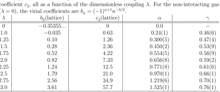
Table 2.1: Fit parameters for the density equation of state, using the functional formn/n0 = 1 + α(βµ)−γ, second-order pressure virial coefficient b2, and leading-order contact virial coefficient c2, all as a function of the dimensionless coupling λ. For the non-interacting gas (λ= 0), the virial coefficients are bn = (−1)n+1n−3/2.
λ b2(lattice) c2(lattice) α γ
0 −0.35355... 0 0.0 −
1.0 −0.035 0.63 0.24(1) 0.46(6)
1.25 0.10 1.26 0.300(5) 0.47(4)
1.5 0.28 2.36 0.450(2) 0.53(9)
1.75 0.52 4.22 0.554(5) 0.56(9)
2.0 0.82 7.33 0.656(8) 0.59(2)
2.25 1.24 12.5 0.771(8) 0.61(6)
2.5 1.79 21.0 0.970(1) 0.66(1)
2.75 2.56 34.9 1.219(6) 0.70(1)
3.0 3.61 57.7 1.525(1) 0.76(1)
and the factor of 1/2 on the left-hand side comes from the number of fermion species. In Table 2.1 we show the virial coefficientb2 obtained by exact diagonalization of the two-body problem on the lattice. The exact result forb2 in the continuum limit, obtained by the same methods utilized in 3D (see e.g. Refs. [28],[29]), is
b2 =−√1 2 +
eλ
2 4
2√2[1 + erf(λ/2)], (2.7)
where erf(x) is the error function. From the above data, we determine other thermodynamic quantities, which furnish a prediction for ultracold atom experiments.
2.3.2: Temperature scale
Having the density as a function ofβµ at our disposal, we can determine the temperature scale in a different convention which is often used, namely T /εF, where εF = k2
F/2 and
kF = πn/2. In Fig. 2.2 we show our results for T /εF as a function of the dimensionless