THE PERFORMANCE OF THE ROBO-AO LASER GUIDE STAR ADAPTIVE OPTICS SYSTEM AT THE KITT PEAK 2.1-M TELESCOPE
Rebecca Jensen-Clem1, Dmitry A. Duev1, Reed Riddle1, Ma¨ıssa Salama2, Christoph Baranec2, Nicholas M. Law3, S. R. Kulkarni1 & A. N. Ramprakash4
1Department of Astronomy, California Institute of Technology, 1200 E. California Blvd., Pasadena, CA 91101, USA 2
Institute for Astronomy, University of Hawai‘i at M¯anoa, Hilo, HI 96720-2700, USA
3Department of Physics and Astronomy, University of North Carolina at Chapel Hill, Chapel Hill, NC 27599-3255, USA 4
Inter-University Centre for Astronomy & Astrophysics, Savitribai Phule Pune University Campus, Pune 411 007, India
ABSTRACT
Robo-AO is an autonomous laser guide star adaptive optics system recently commissioned at the Kitt Peak 2.1-m telescope. Now operating every clear night, Robo-AO at the 2.1-m telescope is the first dedicated adaptive optics observatory. This paper presents the imaging performance of the adaptive optics system in its first eighteen months of operations. For a median seeing value of 1.3100, the average Strehl ratio is 4% in thei0band and 29% in the J band. After post-processing, the contrast ratio under sub-arcsecond seeing for a 2≤i0≤16 primary star is five and seven magnitudes at radial offsets of 0.500 and 1.000, respectively. The data processing and archiving pipelines run automatically at the end of each night. The first stage of the processing pipeline shifts and adds the data using techniques alternately optimized for stars with high and low SNRs. The second “high contrast” stage of the pipeline is eponymously well suited to finding faint stellar companions.
1. INTRODUCTION
Adaptive optics (AO) systems correct wavefront aber-rations introduced by the atmosphere and instrumen-tal optics, restoring the resolution of a telescope to the diffraction limit. Laser guide stars (LGS) were devel-oped in the 1980s to provide AO systems with bright, locatable wavefront reference sources, bringing fainter astrophysical objects into the purview of adaptive op-tics. Over half of all >8-m aperture telescopes are now equipped with an LGS AO system. The primary appli-cation of these AO instruments is for high angular res-olution studies of interesting astronomical objects. As such minimizing the overhead has not been a major con-sideration in the overall design of AO systems on large telescopes.
Robo-AO is a robotic LGS AO system designed for maximum target throughput. Unlike LGS systems on large telescopes, it is based on an artificial star produced by Rayleigh scattering of a near UV laser. Robo-AO achieves high target throughput by minimizing overhead times to less than one minute per target. This is accom-plished by three key design elements: 1) each step of the observation sequence is automated, allowing tasks that would be performed sequentially by a human operator to be performed in parallel and with minimal delay by the robotic system; 2) theλ=355 nm Rayleigh scatter-ing laser guide star is invisible to the human eye. As a
result, while coordination with the U.S. Air Force Joint Space Operations Center (JSpOC) is still required to prevent illumination of sensitive space assets, no con-trol measures are required by the Federal Aviation Ad-ministration; 3) Robo-AO employs an automated queue scheduler which chooses each new science target based on telescope slew times and approved lasing windows provided in advance by JSpOC.
Robo-AO was first commissioned at the Palomar 1.5-m telescope in 2011, where it co1.5-mpleted 19 science runs as a PI instrument from May 2012 through June 2015. Full details of the Robo-AO hardware and software can be found inBaranec et al.(2013),Baranec et al.(2014) andRiddle et al.(2014).
In 2012, the National Optical Astronomy Observatory (NOAO), following the recommendation of the Portfolio Committee which was chartered by the the National Sci-ence Foundation (NSF), decided to divest the Kitt Peak 2.1-m telescope. In 2015, the Robo-AO team made a bid for the telescope and was selected to operate the telescope for three years. Robo-AO was installed at the 2.1-m telescope in November, 2015; since then it has been operating nearly every clear night. As the first dedicated, automated adaptive optics facility, Robo-AO at Kitt Peak is well positioned to support the next gener-ation of large-scale survey programs that are focused on stellar and exoplanet astronomy (e.g. K2, GAIA, CRTS,
Telescope Kitt Peak 2.1-m telescope
Science camera Andor iXon DU-888
EMCCD detector E2V CCD201-20
Read-noise (without EM gain) 47e−
EM gain, selectable 300, 200, 100, 50, 25
Effective read-noise 0.16, 0.24, 0.48, 0.96, 1.9e−
Full-frame-transfer readout 8.6 frames per second
Detector format 10242 13-µm pixels Field of view 3600×3600
Pixel scale 35.1 milli-arcsec per pixel Observing filters g0,r0,i0,z0, lp600
Table 1. The specifications of the Robo-AO optical detector
at Kitt Peak.
PTF, TESS and others), as well as AO follow up of in-teresting sources. Early science results including Robo-AO KP data can be found inAdams et al. (2017) and Vanderburg et al.(2016a,b).
In this paper, we describe the performance of Robo-AO since commissioning. The paper is organized as follows: §2 introduces the Robo-AO imaging systems; §3 provides an overview of our automatic data reduc-tion pipelines; §4 shows the relationships between the weather conditions and the measured seeing;§5presents the Strehl ratio and contrast curve statistics as well as the point spread function (PSF) morphology; §6 de-scribes our automated data archiving system; finally,§7 describes the newly installed near-IR camera.
2. SUMMARY OF THE ROBO-AO IMAGING
SYSTEM
The Robo-AO imaging system includes two optical relays, each using a pair of off-axis parabolic mir-rors. The first relay images the telescope pupil onto a 140-actuator Boston Micromachines micro-electro-mechanical-systems (MEMS) deformable mirror used for wavefront correction. A dichroic then reflects the UV light to an 11×11 Shack-Hartmann wavefront sensor. The second optical relay includes a fast tip-tilt cor-recting mirror and an atmospheric dispersion corrector (ADC; here, two rotating prisms1) located at a reim-aged pupil. The output of the second relay is an F/41 beam that is intercepted by a dichroic mirror, which re-flects the λ < 950 nm portion of the converging beam to the visible wavelength filter wheel and EMCCD de-tector (see Table1). The filter wheel includesg0,r0,i0,
1From the commissioning of Robo-AO at Kitt Peak in Novem-ber of 2015 through February of 2017, the right ascension (RA) axis of the 2.1-m telescope suffered from a∼3.7 Hz jitter (see§5.1 and§A) that caused a slight elongation of the stellar PSFs. As a result, the ADCs were not correctly calibrated until an upgrade to the telescope control system removed the jitter.
and z0 filters, as well as a long-pass “lp600” filter cut-ting on at 600 nm and extending beyond the red limit of the EMCCD (see Figure 1 in Baranec et al. 2014). The dichroic transmits the longer wavelength light to the near-infrared (NIR) instrument port (see§7).
Robo-AO was originally designed for simultaneous op-tical and NIR operations, such that deep science inte-grations could be obtained in one band while the image displacement could be measured in the other and cor-rected with the fast tip-tilt mirror. In February of 2017, we achieved first light with a science-grade novel infrared array, a brief summary of which appears in§72. In this paper, we consider the imaging performance of Robo-AO using the optical imaging camera only. In lieu of an active tip-tilt correction, the EMCCD is run at a fram-erate of 8.6 Hz to allow for post-facto image registration followed by stacking (see§3).
3. DATA REDUCTION PIPELINES
3.1. Overview
Image registration and stacking (see §2) is accom-plished automatically by the “bright star” and “faint star” pipelines, which are optimized for high and low signal-to-noise (SNR) targets, respectively. The data are then processed by the “high contrast” pipeline to maximize the sensitivity to faint companions. These pipelines are described in detail below.
3.2. Image Registration Pipelines
All observations are initially processed by the “bright star” pipeline. This pipeline generates a windowed dat-acube centered on an automatically selected guide star. The windowed region is bi-cubically up-sampled and cross correlated with the theoretical point spread func-tion to give the center coordinates of the guide star’s PSF in each frame. The full-frame, unprocessed images are then calibrated using the nightly darks and dome flats. Finally, the calibrated full frames are aligned us-ing the center coordinates identified by the up-sampled, windowed frames, and co-added via the Drizzle algo-rithm (Fruchter & Hook 2002). These steps are de-scribed in detail inLaw et al. (2014).
After an observation has been processed by the “bright star” pipeline, the core of the brightest star in the frame is fit by a 2D Moffat function. If the full width at half maximum (FWHM) of the function fit to the core is < λ/D, indicating that the stellar centroiding step has failed, the observation is re-processed by the “faint star” pipeline to improve the SNR in the final science image.
The individual frames for a given observation are summed to create a master, dark and flat corrected ref-erence image. This frame is then high pass filtered and windowed about the guide star. Each raw short expo-sure frame is then dark and flat corrected, filtered, and windowed. These individual frames are registered to the master reference frame using the Image Registration for Astronomypython package written by Adam Gins-burg3. The package finds the offset between the individ-ual and reference frames using DFT up-sampling and registers the images with FFT-based sub-pixel image shifts. Figure1illustrates the strengths and weaknesses of the bright and faint star pipelines.
These automatic pipelines have reduced thousands of Robo-AO observations since the instrument was com-missioned in November of 2015. Figure2shows a collage of representative observations.
(a) Bright star, bright star pipeline
(b) Bright star, faint star pipeline
(c) Faint star, bright star pipeline
(d) Faint star, faint star pipeline
Figure 1. The bright star pipeline (a) produces a superior Strehl ratio for the V= 8.84 double star HIP55872 com-pared with (b) the faint star pipeline. For the V= 15.9 star 2MASSJ1701+2621, however, the bright star pipeline (c) fails to correctly center the PSF, leading to an erroneously bright pixel in the center. The faint pipeline (d) successfully shifts and adds this observation.
3.3. High Contrast Pipeline
For science programs that aim to identify point sources at small angular separations from known stars further processing is needed. Our “high contrast imag-ing” pipeline generates a 3.500 frame windowed about the star of interest in the final science frame. A high
3https://github.com/keflavich/image_registration
pass filter is applied to the windowed frame to reduce the contribution of the stellar halo. To whiten corre-lated speckle noise at small angular separations from the target star we subtract a synthetic PSF generated by Karhunen-Lo`eve Image Processing (KLIP). The KLIP algorithm is based on the method of Principal Compo-nent Analysis (Soummer et al. 2012). The PSF diver-sity needed to create this synthetic image is provided by a reference library of Robo-AO observations – a tech-nique called Reference star Differential Imaging (RDI; Lafrenire et al. 2009). We note that the angular differ-ential imaging approach (Marois et al. 2006) is not pos-sible here because the 2.1-m telescope is an equatorial mount telescope. Our pipeline uses the Vortex Image Processing (VIP) package (Gomez Gonzalez et al. 2016).
The full reference PSF library consists of several thou-sand 3.500square high pass filtered frames that have been visually vetted to reject fields with more than one point source. The PSF library is updated on a nightly basis to ensure that each object’s reduction has the opportu-nity to include frames from the same night. Each frame in the full library is cross correlated with the windowed and filtered science frame of interest. The five frames with the highest cross correlation form the sub-library provided to KLIP. We then adopt only the first princi-pal component (PC) as our synthetic PSF, as including more PCs provides no additional noise reduction on av-erage. A future version of the pipeline will choose the number of PCs automatically for each observation based on SNR maximization.
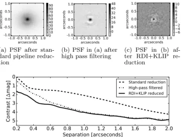
Figure 3 shows an example of a PSF reduced by the standard data pipeline (panel a), then high pass fil-tered (panel b), and finally processed with RDI-KLIP (panelc). After a science frame has been fully reduced we use VIP to produce a contrast curve that is prop-erly corrected for small sample statistics and algorithmic throughput losses. The corresponding contrast curves for the three panels are shown in paneld.
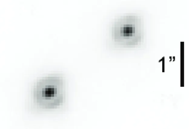
Figure 2. Examples of Robo-AOi0−band images at Kitt Peak (square root scaling) The full-frame (3600×3600) images on the left are the globular cluster Messier 5 (top) and Jupiter (bottom). The images on the right are examples of bright single stars and stellar binaries with a range of separations and contrasts.
(a) PSF after stan-dard pipeline reduc-tion
(b) PSF in (a) after high pass filtering
(c) PSF in (b) af-ter RDI+KLIP re-duction
(d) The dashed, dot-dashed, and solid contrast curves corre-spond to the PSFs shown in (a), (b), and (c), respectively.
Figure 3. An example of the reduction steps in the “high contrast” pipeline for a z0 observation of the star EPIC228859428.
4. SITE PERFORMANCE
4.1. Site Geography
Kitt Peak is located 56 miles southwest of Tucson, Ari-zona, at an elevation of 6800 feet. The 2.1-m telescope is situated 0.4 miles to the south of the peak’s highest point (the location of the Mayall 4-m telescope). The WIYN 3.5-m and 0.9-m telescopes are respectively 700 ft and 400 ft to the west of the 2.1-m telescope and at approx-imately the same elevation. There are no structures at equal or greater elevations to the east of the telescope, and the terrain is relatively flat beyond Kitt Peak in that direction. The 7730 ft Baboquivari Peak is 12 miles directly south of the telescope.
4.2. Seeing Measurement
registra-tion of the individual exposures. The seeing is defined as the FWHM of a two-dimensional Gaussian function fit to this summed frame. Starting in January of 2017, a 90 s seeing observation was obtained each hour. Specifi-cally, the Robo-AO queue schedules an observation of a bright (V < 8) star within 10◦ of zenith to refocus the telescope and measure the seeing. As of this writing, there is no significant difference between these “long” and “short” seeing observations. Here on we proceed with the assumption that the 10 s seeing measurements are representative of the long-exposure seeing.
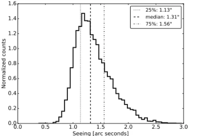
We display a histogram of these fiducial seeing values in Figure5. Figure4displays the seeing as a function of the seasons. The seeing values measured in a given wave-length are scaled to a fiduciary wavewave-length of 500 nm by the scaling law seeing500 nm=seeingλ× (λ/500 nm)1/5.
4.3. Seeing Contributions
We note that our median seeing of 1.3100differs from the median seeing of 0.800 reported by the adjacent WIYN telescope4. One possible explanation for this dis-crepancy is that the WIYN was built in 1994 with careful attention paid to dome ventilation and telescope ther-mal inertia. In contrast, the 2.1-m telescope saw first light in 1964 before such considerations were fully appre-ciated. Figure 6 demonstrates the challenging thermal conditions at the 2.1-m telescope: during the majority of Robo-AO observations, the mirror is warmer than the ambient dome temperature which in turn is warmer than the outside air. The experience of other observatories indicate that improvements to dome thermalization can significantly improve the measured seeing (e.g.Bauman et al. 2014).
Another possible cause of the comparatively poor see-ing at the 2.1-m telescope is perhaps a more turbu-lent ground layer. Figure 7 shows a “wind rose,” or the frequency of wind speeds originating from differ-ent directions, for December 2015 through June 2016. We find that during this period the wind most com-monly blows from the NNW, or the direction of the higher elevation Mayall 4-m telescope, and rarely from the SE where the terrain is less mountainous. The high-est winds (> 40 mph) come from the north while the south has the largest fraction of low wind speeds (the wind speeds originating from within 20◦ of due south are under 10 mph 73% of the time).
Despite these terrain variations, the seeing is not sig-nificantly correlated with the wind direction. The wind speed, however, degrades the seeing by several tenths of an arcsecond for winds over 20 mph (the dome closes for winds over 40 mph).
4https://www.noao.edu/wiyn/aowiyn/
Figure 8 plots the seeing versus the wind speed, demonstrating that poorer seeing is correlated with higher wind speeds5. We note that the wind monitor became nonfunctional after June of 2016, and hence fur-ther study of the relationship between the seeing and the wind speed will occur after a new wind monitor is in place.
5. ADAPTIVE OPTICS PERFORMANCE
5.1. Strehl Ratio
The goal of an adaptive optics system is to bring the observed PSF closer to its theoretical diffraction-limited shape; hence, an important measure of the AO system’s performance is the ratio between the peak intensity of an observed PSF and that of the telescope’s theoretical PSF – the Strehl ratio. As the AO performance improves, the Strehl ratio increases.
We calculate the Strehl ratio by 1) generating a monochromatic diffraction-limited PSF by Fourier transforming an oversampled image of the pupil, 2) com-bining several monochromatic PSFs to create a PSF representative of the desired bandpass, 3) re-sampling the polychromatic PSF to match our 0.017500/pixel platescale of the up-sampled “drizzled” frames, 4) ob-taining the “Strehl factor,” or the ratio of the peak in-tensity to the sum of the inin-tensity in a 300square box, and 5) calculating the Strehl ratio by repeating step 4 for the observed image and dividing by the Strehl fac-tor. These steps are described in detail inSalama et al. (2016).
Once Robo-AO began regular observations at the 2.1-m telescope, we noticed that the achieved Strehl ratios were noticeably smaller than those that were achieved (for similar seeing values) at the Palomar 1.5-m tele-scope. A number of exercises were undertaken to de-termine possible causes for this degradation. Eventu-ally, we determined that the Telescope Control System (TCS) was the main contributing factor. In Appendix Awe discuss the problem in detail. The mitigation con-sisted of upgrading the TCS (completed February 2017). Below, and for the rest of the paper, we discuss the in-strument performance since the TCS upgrade.
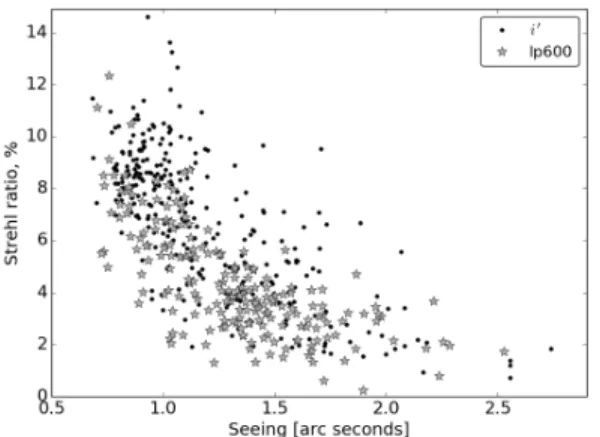
Figure 9 plots the Strehl ratio versus the measured seeing for the i0 and lp600 filters. It is clear that the delivered Strehl ratio drops off quickly as the seeing in-creases – while Robo-AO achieves > 10% Strehl ratio when the seeing is<1.000, a 0.2500seeing increase halves the Strehl ratio.
Figure 4. Seasonal fiducial (λ =500 nm; see §4.2) seeing measurements. Nightly median values were used to fit a monthly distribution. The fraction of nights with seeing data for each month is shown. The quartile values and the actual measured range are shown.
0.0 0.5 1.0 1.5 2.0 2.5 3.0
Seeing [arc seconds] 0.0
0.2 0.4 0.6 0.8 1.0 1.2 1.4 1.6
Normalized counts
25%: 1.13" median: 1.31" 75%: 1.56"
Figure 5. A histogram of the seeing measurements (all ref-erenced to a wavelength λ =500 nm) from December 2015 to March 2017. A zenith distance dependent correction has been applied. The 25th, 50th, and 75th percentile seeing values are indicated by the vertical lines.
3 2 1 0 1 2 3
Temperature Difference [◦C] 0.0
0.2 0.4 0.6 0.8 1.0 1.2
Frequency
Primary - Dome Dome - Outside
Figure 6. Histograms of the difference between the primary mirror and dome temperatures (solid) and the dome temper-ature minus the outside air tempertemper-ature (dashed).
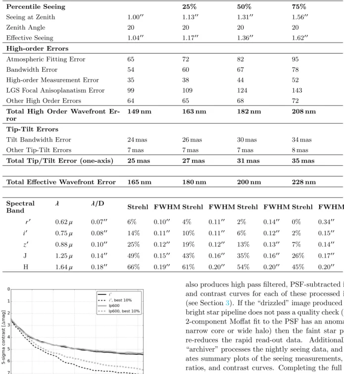
In Table 2 we present a detailed error budget under different seeing conditions. This error budget was origi-nally developed by R. Dekany (private communication), and was validated against the on-sky performance of laser AO systems on the Keck telescope, the Hale
tele-0.4” – 0.7” 0.7” – 1.0” 1.0” – 1.4” 1.4” – 1.7” 1.7” – 2.0” > 2.0” 1.4 – 9.4 mph
9.4 – 17.3 mph 17.3 – 25.3 mph 25.3 – 33.2 mph 33.2 – 41.2 mph > 41.2 mph
0.6% - 2.5% 2.5% - 4.4% 4.4% - 6.3% 6.3% - 8.2% 8.2% - 10.2% > 10.2%
Figure 7. A “wind rose” showing a stacked polar histogram of wind speeds and directions from December 2015 through June 2016. The wind most frequently blows from the NW, N, and NE, which correspond to the more mountainous region towards the direction of the Mayall 4-m telescope. These also tend to be the direction of the high wind speeds while slower wind speeds most often come from the south, where the terrain is less mountainous.
scope and the Palomar 1.5-m telescope (Baranec et al. 2012). Since we lacked turbulence profile(s) for the 2.1-m telescope site we adopt a 2.1-meanC2
n(h) profile from a MASS-DIMM atmospheric turbulence monitor collected over a year’s baseline at Palomar and scaled to the see-ing at Kitt Peak.
quadra-0 5 10 15 20 25 30 35 Wind Speed [mph]
1.4 1.5 1.6 1.7 1.8 1.9
Seeing [arc seconds]
Figure 8. The mean binned seeing versus the wind speed for December 2015 through June 2016. The error bars are the standard deviation of the seeing values in a given wind speed bin divided by the square root of the number of seeing measurements in the bin. For wind speeds over 20 mph, the seeing is degraded by up to 0.300
.
ture with the high-order errors. Other high-order and tip-tilt errors include chromatic, scintillation, aliasing, calibration and digitization errors.
Strehl ratios are calculated using the Mar´echal approximation. The full-widths at half-maximum (FWHM) are calculated from PSF models assuming the residual diffraction-limited, concentrated light, residual seeing, and scattered light halos are proportional to the phase variance of the residual errors. These models have shown accuracy of a few percent for Strehl ratios as low as 4% (Sheehy et al. 2006). Figure9demonstrates Robo-AO’s ability to approach the predicted Strehl ratio of 14% in sub-arcsecond seeing conditions.
Figure 9. The Strehl ratio versus the measured seeing values for 21 February 2017 through 10 March 2017 in thei0 and lp600 filters.
5.2. PSF Morphology
Figure 10 shows a representative Robo-AO point spread function (PSF) corresponding to the V=10 star
HIP56051. The observation was taken in the i0 band with a total exposure time of 90 s. The seeing at the time of the observation was 0.9400, and the Strehl ratio of the final PSF is 10.17%.
-1.0 -0.5 0.0 0.5 1.0
Separation [arcseconds] 0
5 10 15 20
Counts
Stellar PSF Moffat Fit to Core Moffat Fit to Halo Gaussian Seeing Disk
0.5
1.0
1.5 2.0 2.5 3.0
∆
M
ag
nit
ud
e
Figure 10. A 1D cut through the PSF of HIP56051 is plotted with two Moffat functions fit to the PSF core and halo, re-spectively. The dashed curve is a Gaussian distribution with a FWHM corresponding to the seeing measurement and an area equal to the observed PSF’s area.
The effect of the AO system is to re-arrange the starlight from the equivalent area seeing-limited PSF (dashed curve) to the sharper, observed PSF plotted by the black points. The AO-corrected PSF includes two components: a sharp core and a broader halo, each separately fit by Moffat functions (the light and dark gray curves, respectively). The full width at half maxi-mum (FWHM) of the Moffat function fit to the core is 0.100±0.0100. This value is consistent with the diffraction limit of 1.028λ/D=0.0800.
5.3. Contrast Curves
Section §3 described the “high contrast pipeline,” which produces 5σ contrast curves from the high pass filtered, RDI-PCA reduced science frames. Figure 11 plots the median and best 10% contrast curves for i0 and lp600 filter science frames. Under sub-arcsecond seeing (the best 10% of cases), the contrast ratio for a 2≤i0≤16 primary star is five and seven magnitudes at 0.500 and 1.000, respectively.
6. DATA ARCHIVE
We have developed a fully automated data processing and archiving system6. The data reduction chain for an observing night proceeds as follows. At the end of each night, the visual camera data are compressed and trans-ferred to the network storage. Next, the darks and dome
Table 2. The Robo-AO Error Budget
Percentile Seeing 25% 50% 75%
Seeing at Zenith 1.0000 1.1300 1.3100 1.5600
Zenith Angle 20 20 20 20
Effective Seeing 1.0400 1.1700 1.3600 1.6200
High-order Errors
Atmospheric Fitting Error 65 72 82 95
Bandwidth Error 54 60 67 78
High-order Measurement Error 35 38 44 52
LGS Focal Anisoplanatism Error 99 109 124 143
Other High Order Errors 64 65 68 72
Total High Order Wavefront Er-ror
149 nm 163 nm 182 nm 208 nm
Tip-Tilt Errors
Tilt Bandwidth Error 24 mas 26 mas 30 mas 34 mas
Other Tip-Tilt Errors 7 mas 7 mas 7 mas 8 mas
Total Tip/Tilt Error (one-axis) 25 mas 27 mas 31 mas 35 mas
Total Effective Wavefront Error 165 nm 180 nm 200 nm 228 nm
Spectral Band
λ λ/D
Strehl FWHM Strehl FWHM Strehl FWHM Strehl FWHM
r0 0.62µ 0.0700 6% 0.1000 4% 0.1100 2% 0.1400 0% 0.3400
i0 0.75µ 0.0800 14% 0.1100 10% 0.1100 6% 0.1200 2% 0.1500
z0 0.88µ 0.1000 25% 0.1200 19% 0.1200 13% 0.1300 7% 0.1400
J 1.25µ 0.1400 49% 0.1500 43% 0.1600 35% 0.1600 26% 0.1700
H 1.64µ 0.1800 66% 0.1900 61% 0.2000 54% 0.2000 45% 0.2000
Figure 11. The contrast as a function of distance from the central star for the i0 and lp600 filters. The dashed lines show the best 10% contrast curves for each filter.
flats taken at the beginning of each night are combined into master calibration files and applied to the obser-vations. The bright star pipeline is then run on each observation followed by the computation of the Strehl ratio of the resulting image. The high contrast pipeline
also produces high pass filtered, PSF-subtracted images and contrast curves for each of these processed images (see Section3). If the “drizzled” image produced by the bright star pipeline does not pass a quality check (i.e. if a 2-component Moffat fit to the PSF has an anomalously narrow core or wide halo) then the faint star pipeline re-reduces the rapid read-out data. Additionally, the “archiver” processes the nightly seeing data, and gener-ates summary plots of the seeing measurements, Strehl ratios, and contrast curves. Completing the full reduc-tion chain for a typical night’s worth of data takes a few hours.
The “house-keeping” system uses a Redis7-based
hueypython package8to manage the processing queue, which distributes the jobs to utilize all available compu-tational resources. The processing results together with ancillary information on individual observations and
7An efficient in-memory key-value database
system performance are stored in a MongoDB9 NoSQL database. For interactive data access, we developed a web-based interface powered by the Flask10 back-end. It allows the user to access previews of the processing results together with auxiliary data (e.g. external VO images of a field), nightly summary and system perfor-mance information. The web application serves as the general interface to the database providing a sophisti-cated query interface and also has a number of analysis tools.
7. NEAR-INFRARED CAMERA
In November 2016, we installed a NIR camera for use with Robo-AO. While similar to the camera deployed in engineering tests at the Palomar 1.5-m telescope in 2014 (Baranec et al. 2015), the new camera uses a science-grade detector and faster readout electronics. The de-tector is a Mark 13 Selex ES Advanced Photodiode for High-speed Infrared Array (SAPHIRA) with an ME-911 Readout Integrated Circuit (Atkinson et al. 2016;Baker et al. 2016). It has sub-electron readnoise and 320× 256-pixel array with λ = 2.5µm cutoff. The single-board PB1 ‘PizzaBox’ readout electronics were developed at the Institute for Astronomy and we use 32 readout chan-nels, each capable of a 2 Mpixel/sec sampling rate, for a maximum full-frame read rate of∼800Hz.
The NIR camera attaches to the Robo-AO f/41 in-frared camera port that accessesλ >950nm after trans-mission through a dichroic. The camera has an internal coldλ <1.85µm short-pass filter and an external warm filter wheel with J, H, clear, and blocking filters. The camera has a plate scale of 0.06400 per pixel and field-of-view of 16.500×20.600.
We achieved first light on sky in February 2017 dur-ing final testdur-ing of the upgraded TCS. Initially we used a 1 Mpixel/sec sampling rate (a full frame read rate of 390 Hz) with detector resets every 300 reads. To create a reduced image, we first assembled difference frames between 39 consecutive reads, totaling∼0.1 s of integra-tion time, short enough to effectively freeze stellar image displacement. We subtracted a frame median to approx-imate removing the background. We then synthesized a long exposure image by registering each corrected frame on the brightest target in the field. Figure12shows an example image of a binary star observed in H-band.
For the moment, data acquisition and reduction is per-formed manually. In the coming months, we will opti-mize the detector readout routines for maximum sen-sitivity to faint objects (including dithering for back-ground removal), integrate the operation of the camera
9
https://www.mongodb.com
10https://github.com/pallets/flask
Figure 12. A 5.5 s image of GJ1116 taken in H-band with
the near-infrared camera (linear stretch).
into the robotic queue and modify our existing data re-duction pipeline to handle the NIR data. We will also investigate automating active tip-tilt correction by using either the visible or infrared camera as a tip-tilt camera, as previously demonstrated at Palomar.
8. CONCLUSION
Robo-AO at the Kitt Peak 2.1-m telescope is the first dedicated adaptive optics observatory. Observing every clear night, Robo-AO has the capacity to undertake LGS AO surveys of large samples. For instance, a 1000-star survey with exposure times of 60 s per target can be completed on the timescale of a week.
Science programs designed to exploit Robo-AO’s unique capabilities are underway. These programs in-clude stellar multiplicity in open clusters, minor planet binarity, major planet weather variability, extragalac-tic object morphology, sub-stellar companions to nearby young stars, M-star multiplicity, and the influence of stellar companions on asteroseismology. By the summer of 2017, Robo-AO will become the first LGS AO system to operate entirely autonomously, as on-going upgrades to the 2.1-m telescope will remove the need for a human observer.
Na-tional Science Foundation under grants AST-0906060, AST-0960343, and AST-1207891, IUCAA, the Mt. Cuba Astronomical Foundation, and by a gift from Samuel Oschin. These data are based on observations at Kitt Peak National Observatory, National Optical Astron-omy Observatory (NOAO Prop. ID: 15B-3001), which
is operated by the Association of Universities for Re-search in Astronomy (AURA) under cooperative agree-ment with the National Science Foundation. C.B. ac-knowledges support from the Alfred P. Sloan Founda-tion.
Facility:
KPNO:2.1m (Robo-AO)REFERENCES
Adams, E. R., Jackson, B., Endl, M., et al. 2017,The Astronomical Journal, 153, 82
Atkinson, D. E., Hall, D. N. B., Baker, I. M., et al. 2016,in Proc. SPIE, Vol. 9915, Society of Photo-Optical
Instrumentation Engineers (SPIE) Conference Series, 99150N Baker, I., Maxey, C., Hipwood, L., & Barnes, K. 2016,in
Proc. SPIE, Vol. 9915, Society of Photo-Optical
Instrumentation Engineers (SPIE) Conference Series, 991505 Baranec, C., Atkinson, D., Riddle, R., et al. 2015,The
Astrophysical Journal, 809, 70
Baranec, C., Riddle, R., Ramaprakash, A. N., et al. 2012,in Proc. SPIE, Vol. 8447, Adaptive Optics Systems III, 844704 Baranec, C., Riddle, R., Law, N. M., et al. 2013,Journal of
Visualized Experiments
—. 2014,The Astrophysical Journal Letters, 790, L8 Bauman, S. E., Benedict, T., Baril, M., et al. 2014,in
Proc. SPIE, Vol. 9149, Observatory Operations: Strategies, Processes, and Systems V, 91491K
Fruchter, A. S., & Hook, R. N. 2002,Publications of the Astronomical Society of the Pacific, 114, 144
Gomez Gonzalez, C. A., Absil, O., Absil, P.-A., et al. 2016, Astronomy and Astrophysics, 589, A54
Hardy, J. W. 1998, Adaptive Optics for Astronomical Telescopes, Oxford Series in Optical and Imaging Sciences (Oxford, New York: Oxford University Press)
Lafrenire, D., Marois, C., Doyon, R., & Barman, T. 2009,The Astrophysical Journal Letters, 694, L148
Law, N. M., Baranec, C., & Riddle, R. L. 2014,in Proc. SPIE, Vol. 9148, Adaptive Optics Systems IV, 91480A
Marois, C., Lafrenire, D., Doyon, R., Macintosh, B., & Nadeau, D. 2006,The Astrophysical Journal, 641, 556
Riddle, R. L., Hogstrom, K., Papadopoulos, A., Baranec, C., & Law, N. M. 2014,in Proc. SPIE, Vol. 9152, Software and Cyberinfrastructure for Astronomy III, 91521E
Salama, M., Baranec, C., Jensen-Clem, R., et al. 2016,in Proc. SPIE, Vol. 9909, Society of Photo-Optical
Instrumentation Engineers (SPIE) Conference Series, 99091A Sheehy, C. D., McCrady, N., & Graham, J. R. 2006,ApJ, 647,
1517
Soummer, R., Pueyo, L., & Larkin, J. 2012,The Astrophysical Journal Letters, 755, L28
Vanderburg, A., Becker, J. C., Kristiansen, M. H., et al. 2016a, The Astrophysical Journal Letters, 827, L10
Vanderburg, A., Bieryla, A., Duev, D. A., et al. 2016b,The Astrophysical Journal Letters, 829, L9
APPENDIX
A. TELESCOPE JITTER
After moving Robo-AO from the Palomar 1.5-m telescope to the Kitt Peak 2.1-m telescope, the median Strehl ratio across all wavelengths was initially reduced from 5.8% to 3.2%. The source of this degradation was a∼3.7 Hz vibration in the RA axis. Because Robo-AO mitigates tip/tilt by post facto shift and add rather than a real-time loop, and because its framerate is typically only 8.6 Hz, the targets were smeared in the RA direction. Figure A1a and b show the power spectral densities of the mean subtracted RA centroid positions of targets observed at Kitt Peak and Palomar, respectively. The peak at ∼3.7 Hz is clear in the Kitt Peak data, but is not present at Palomar. The RA-axis smearing for a single test observation is demonstrated in FigureA2.
(a) Kitt Peak mean subtracted RA centroids (b) Palomar mean subtracted RA centroids
Figure A1. The power spectral densities of the mean subtracted RA target positions for each sub-exposure at Kitt Peak (a) and Palomar (b). The peak at∼3.7 Hz is present at Kitt Peak, but not at Palomar. The solid black lines show the theoretical
power-law dependencies of the tilt: f−2/3at low frequencies, and f−2 for 1−10 Hz (Hardy 1998).
250 200 150 100 50 0
Angle [Degrees]
2 4 6 8 10 12 14 16 18 20
Pixels
Semi-Major Axis Semi-Minor Axis
Figure A2. For a test observation, the standard deviation along the semi-major and semi-minor axes of 2D Gaussian fits to each 0.116s sub-exposure are plotted versus the rotation angle of the Gaussian. Here,−90◦ (dashed black line) indicates that the semi-major axis lies along the RA-axis. Clearly, the PSF is elongated along the RA-axis.
0.5 1.0 1.5 2.0 2.5 Seeing [arc seconds] 0
2 4 6 8 10 12 14
Strehl ratio, %
i0, Before Upgrade
i0, After Upgrade