Cover Page
The handle http://hdl.handle.net/1887/24481
holds various files of this Leiden University
dissertation
Author
: Bamakhrama, Mohamed A.
Title
: On hard real-time scheduling of cyclo-static dataflow and its application in
system-level design
On Hard Real-Time Scheduling of Cyclo-Static Dataflow
and its Application in System-Level Design
On Hard Real-Time Scheduling of Cyclo-Static Dataflow and
its Application in System-Level Design
PROEFSCHRIFT
ter verkrijging van
de graad van Doctor aan de Universiteit Leiden, op gezag van Rector Magnificus prof.mr. C.J.J.M. Stolker,
volgens besluit van het College voor Promoties te verdedigen op woensdag 12 maart 2014
klokke 15:00 uur
door
Mohamed Ahmed Mohamed Bamakhrama geboren te Dubai
Promotion Committee
Promotor: Prof. dr. Ed F. Deprettere Universiteit Leiden Co-Promotor: Dr. Todor P. Stefanov Universiteit Leiden Other Members: Prof. dr. Petru Eles Linköpings Universitet
Prof. dr. Rolf Ernst Technische Universität Braunschweig Prof. dr. Marco Bekooij Universiteit Twente
Prof. dr. Joost Kok Universiteit Leiden Prof. dr. Farhad Arbab Universiteit Leiden Prof. dr. Harry Wijshoff Universiteit Leiden
On Hard Real-Time Scheduling of Cyclo-Static Dataflow and its Application in System-Level Design
Mohamed A. Bamakhrama.
-Dissertation Universiteit Leiden. - With ref. - With summary in Dutch.
Copyright © 2014 by Mohamed A. Bamakhrama. All rights reserved.
This dissertation is licensed under the Creative Common Attribution-Share Alike 3.0 license. You can obtain a copy of this license from the following URL:
http://creativecommons.org/licenses/by-sa/3.0/
This dissertation was typeset using LATEX and version controlled using Git.
My prayer and my sacrifice and my life and my death are all for God, the Lord of the worlds.
Contents
Table of Contents vii
List of Figures xi
List of Tables xiii
1 Introduction 1
1.1 Current Design Challenges and Trends . . . 3
1.1.1 Design of Concurrent Software . . . 4
1.1.2 Designer Productivity . . . 6
1.1.3 Real-Time Guarantees . . . 8
1.2 Problem Statement . . . 10
1.3 Research Contributions . . . 11
1.4 Related Work . . . 13
1.4.1 Hard Real-Time Scheduling of Streaming Programs . . . 14
1.4.2 Design Flows for Hard Real-Time Streaming Systems . . . 19
1.5 Organization of this Dissertation . . . 20
2 Background 23 2.1 Notations . . . 23
2.2 Parallel Execution of Programs . . . 23
2.3 Cyclo-Static Dataflow (CSDF) . . . 26
2.4 Real-Time Scheduling . . . 29
2.4.1 Task Model . . . 29
2.4.2 Scheduling Concepts . . . 30
2.4.3 Uniprocessor Schedulability Analysis . . . 32
viii Contents
3 Automated Parallelization and Model Construction 39
3.1 Input Programs . . . 39
3.1.1 Top-Level Part . . . 39
3.1.2 Implementation Part . . . 40
3.2 Automated Parallelization . . . 41
3.3 Model Construction . . . 42
4 Scheduling Framework 47 4.1 Input Streams . . . 48
4.2 Basic Definitions . . . 50
4.3 Deriving Periods . . . 52
4.4 Deriving Deadlines and Start Times . . . 57
4.5 Deriving Buffer Sizes . . . 61
4.6 Throughput Analysis . . . 65
4.7 Latency Analysis . . . 67
4.8 Deriving Architecture and Mapping Specifications . . . 70
5 System-Level Synthesis 75 5.1 Hardware . . . 75
5.2 Software . . . 77
5.2.1 Scheduling Infrastructure . . . 78
5.2.2 Communication Infrastructure . . . 83
6 Evaluation and Results 87 6.1 Experiment I: Evaluating Automated Parallelization and Model Con-struction . . . 88
6.2 Experiment II: Evaluating Performance and Resource Usage Metrics under Periodic Scheduling . . . 88
6.2.1 Benchmarks . . . 89
6.2.2 Throughput Evaluation . . . 89
6.2.3 Latency Evaluation . . . 90
6.2.4 Processor Requirements Evaluation . . . 91
6.2.5 Memory Requirements Evaluation . . . 93
6.2.6 Summary of Experiment II . . . 93
6.3 Experiment III: Validating Synthesized Systems . . . 95
7 Summary and Future Work 99 7.1 Suggestions for Future Work . . . 101
Contents ix
Curriculum Vitae 119
List of Publications 120
Samenvatting 121
List of Figures
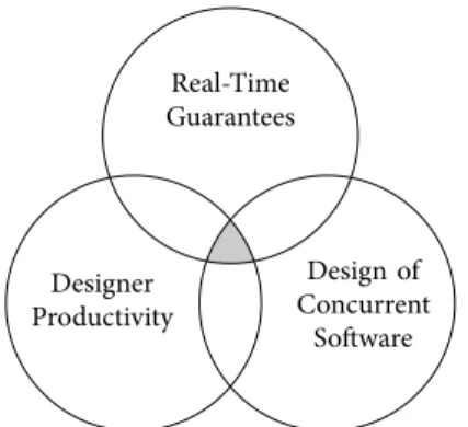
1.1 The challenges involved in designing modern hard real-time
multipro-cessor streaming systems. . . 4
1.2 Decidability and expressiveness for popular dataflow MoCs . . . 6
1.3 System-level design of modern embedded systems . . . 7
1.4 Popular real-time task models and the complexity of their feasibility tests 9 1.5 Bridging dataflow MoCs and real-time task models through the pro-posed scheduling framework . . . 11
1.6 Input and outputs of the proposed scheduling framework . . . 12
1.7 Overview of the proposed design flow . . . 14
2.1 Example of a CSDF graph that corresponds to the SANLP program in Listing 1 . . . 29
3.1 Automated parallelization and model construction . . . 40
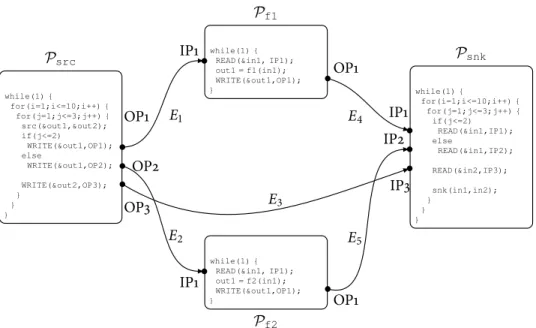
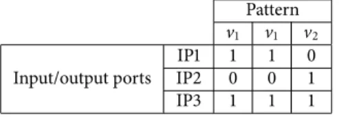
3.2 The parallel program corresponding to the SANLP shown in Listing 1 42 3.3 The port domains of𝒫snkshown in Figure 3.2 . . . 43
3.4 The domains ofv1andv2 . . . 44
4.1 Scheduling framework . . . 48
4.2 Occurrence oftMIT(Ii,j) . . . 49
4.3 Computingtbuffer(Ii,j) . . . 49
4.4 ScheduleS1 . . . 55
4.5 ScheduleS2 . . . 55
4.6 ScheduleSL. . . 55
4.7 ScheduleS∞ . . . 56
4.8 The periodic schedule for the CSDF graph shown in Figure 2.1 con-structed using Theorem 4.3.1 . . . 57
4.9 Timeline ofAiandAjwhent′≥Si . . . 60
4.10 Timeline ofAiandAjwhent′<Si . . . 60
xii List of Figures
4.12 Execution time-lines ofAiandAjwhenSi>Sj . . . 63
4.13 Decision tree for scheduling CSDF actors as real-time periodic tasks 71 4.14 The CSDF graph corresponding to the SANLP program shown in Listing 2 . . . 72
4.15 Mapping ofG1andG2onto 6 processors assuming EDF and FFD . . 73
5.1 Electronic System-Level Synthesis . . . 76
5.2 Top-level block diagram of the hardware platform considered in this dissertation . . . 76
5.3 Tile organization . . . 77
5.4 Complete MPSoC architecture . . . 78
5.5 Crossbar Topology . . . 79
5.6 Detailed description of functionvTaskDelayUntil . . . 81
5.7 FIFO layout in memory and the read/write registers . . . 83
6.1 Results of the latency evaluation . . . 92
6.2 Minimum number of processors required by optimal and partitioned schedulers . . . 94
List of Tables
2.1 Summary of mathematical notations . . . 24 2.2 Approximation rations for known bin packing heuristics . . . 37
3.1 Deriving production/consumption rates sequences from the shortest repetitive pattern . . . 45
4.1 ComputingD⃗andS⃗for the CSDF graph shown in Figure 2.1 on page
29 under different values ofη⃗. . . 61
4.2 Computing the buffer sizes for the CSDF graph shown in Figure 2.1 on page 29 under different values ofη⃗. . . 64
4.3 Values ofKui andKuj defined in (4.49) and (4.50) for the CSDF graph shown in Figure 2.1. . . 68 4.4 The output paths latencies and graph maximum latency of the CSDF
graph shown in Figure 2.1 on page 29 under different values ofη⃗. . . . 68
4.5 The taskset parameters forG1andG2assumingµG =1 andη⃗= ⃗1 for
both graphs . . . 72
6.1 Specifications of the machine on which the experiments were performed 87 6.2 Time needed to parallelize and derive the CSDF model for the
bench-mark programs . . . 88 6.3 Benchmarks used for evaluating the periodic scheduling framework
proposed in Chapter 4 . . . 90 6.4 Results of Throughput Comparison . . . 91 6.5 The total amount of memory needed to realize the buffers in the
Chapter 1
Introduction
The computer was born to solve problems that did not exist before.
Bill Gates
T
HE current period of human history is known as theinformationage. This name stems from the fact that humanity is shifting from the traditional industry-based society that characterized the industrial revolution period between 1700-1900 CE, into aknowledge-based society. The knowledge which used to be concentrated only in libraries and accessible only to a small fraction of the society has now become available (mostly for free) to anyone with a computer and Internet access. This dissemination of knowledge has been mainly enabled by the advent ofelectronic computersand all the advances that they enabled and brought such as the Internet. Electronics in general, and computers in particular, have changed many aspects in our behavior and way of thinking. Today, computers resemble the “backbone” of a modern society. They are everywhere starting from mobile phones and MP3 players and all the way to satellites, airplanes, and nuclear reactors. They process daily vast amounts of data to ensure that our societies continue to function properly. Computer systems can be classified based ontheir functionalityinto two categories:1. General-purposesystems such as Personal Computers (PC). Such systems are flexible and can be controlled directly by the user to perform a variety of tasks such as web browsing, word processing, gaming, etc.
2. Embeddedsystems such as the ones that you can find inside digital TVs, cars, trains, etc. Such systems have specific functionality and they are mostly invisible to the user. Such computer systems are said to be embeddedwithin larger systems.
2 Chapter 1. Introduction
life. However, almost 90% of all computer systems shipped worldwide in 2010 were actually embedded systems [MRP+11]. Embedded systems have become pervasive in our life. They are everywhere, and even though that we mostly do not see them, we still feel their presence through their actions. A very important property of embedded systems is that their correct functionality does not depend only on producing the correct result but also on producing the correct resultat the right time. Such systems, where time is critical to the correct functionality, are calledreal-time systems. Real-time systems can be eitherhardorsoft. A hard real-time system is one where the failure to meet the timing requirements leads to a systemfailure. In contrast, a soft real-time system is one where the failure to meet the timing requirements does not lead to a failure but todegradedsystem performance that can be tolerated. Deciding whether a system is hard or soft depends usually on the overall system requirements and the environment where the system is deployed.
Real-time systems can be further classified, based on thetype of programsthey run, into:
1. Controlprograms that wait for external events from the physical world, and then react to these events. Examples include factory automation programs running on Programmable Logic Controllers (PLC) and railway switching systems.
2. Streamingprograms that are characterized by processing continuousstreamsof data which arrive to the system. Usually, such programs process large amounts of data within short periods of time. Examples of such programs include those used in video and audio processing, digital signal processing, and network protocol processing.
In many cases, a single embedded system can contain both control and streaming programs.
1.1. Current Design Challenges and Trends 3
designing such systems and their implications.
1.1
Current Design Challenges and Trends
As general-purpose computers have moved from single core processors to multicore processors [HNO97], the same has happened in the embedded systems domain. Today, embedded systems designers integrate multiple processors, hardware peripherals and memories into a single chip. Such chips are referred to asMultiprocessor System-on-Chip (MPSoC)[JTW05]. MPSoCs represent a good candidate for running many computationally-intensive streaming programs in hard real-time systems. For example, Thrun reported in [Thr10] that Stanford’s Stanley self-driving car, which was used in DARPA 2005 challenge, employed two Intel quad-core processors in order to run the autonomous driving software, including path planning and collision avoidance algorithms. Such algorithms are also highly parallelizable [KKLR13], which means that they benefit from execution on multiprocessor systems. However, such algorithms are specified, most of the time, as sequential programs. This means that such programs must be parallelized in order to meet their timing constraints and utilize the underlying processors. Another challenge is that designing MPSoCs is becoming increasingly complex as the number of processors integrated onto a single chip keeps increasing. According to the International Technology Roadmap for Semiconductors (ITRS) report for 2011 [Int11]:
“In the near term, the grand challenges for design technology remain (1) power management, and (2) design productivity and design for manufacturability. In the long term, the grand challenges for design technology have been up-dated as (1) design of concurrent software, and (2) design for reliability and resilience.”
4 Chapter 1. Introduction
Real-Time Guarantees
Designer Productivity
Design of Concurrent
Software
Figure 1.1:The challenges involved in designing modern hard real-time multiprocessor streaming
systems.
1.1.1 Design of Concurrent Software
Software became a very important component in modern embedded systems. The amount and complexity of software that is running on such systems has increased dramatically over the last decades. For example, the size of embedded software in automotive systems has increased by two orders of magnitude between 1990 and 2010 [EJ09]. According to [EJ09], software is becoming a key differentiator in many domains such as automotive. A complicating factor in designing modern embedded systems is that embedded software must be written asparallelsoftware in order to utilize the underlying processors in an MPSoC. Given a sequential program, researchers have identified three possible types of parallelism:
1. Instruction-LevelParallelism (ILP): this represents the lowest level of paral-lelism that is visible to the programmer. Under ILP, multiple instructions within the program may be executed in parallel.
2. Data-LevelParallelism (DLP): under DLP, a function (or block) within the program is executed simultaneously on several processors and each copy of the function processes its own stream of data.
3. Task-LevelParallelism (TLP): under TLP, the program is split into a set of functions (ortasks) and these functions execute in parallel.
1.1. Current Design Challenges and Trends 5
multiprocessor systems. Traditionally, embedded software has been designed at the level of Board Support Package (BSP) and high-level Application Programming Inter-face (API) [HHBT09]. An example of a popular API for designing concurrent software is the POSIX threads (Pthreads) standard [SG13]. However, designing concurrent software at this level is known to be a cumbersome and error-prone task and it is not easy to provide timing guarantees [Lee06]. Therefore, it has been recognized that the designers need to abstract from the actual programs by buildinghigh-level modelsof them [EJ09, Tei12]. Then, these models are used to analyze the program performance under different scheduling and mapping decisions. Such design approach is often called Model-Based Design (MBD)orModel-Driven Design (MDD)and the models used in such approaches are calledModels of Computation (MoC)[HHBT09].
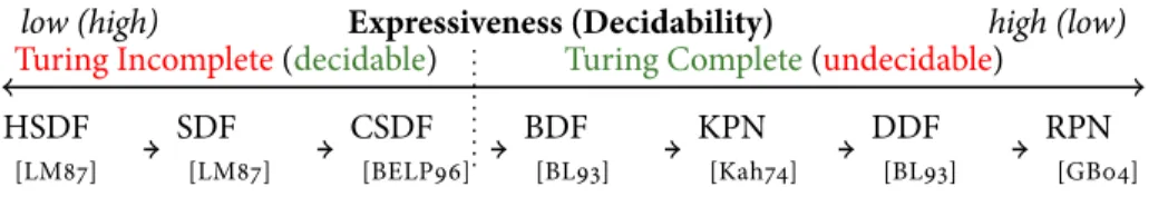
In the broadest sense, a MoC defines the set of permitted operations used in com-putation. MoCs can be classified as eithersequentialorparallel. In this dissertation, we are interested in parallel MoCs as they are suitable for expressing programs that are mapped onto MPSoCs. In particular,dataflowMoCs have been identified as suitable parallel MoCs for expressing streaming programs [TA10]. In general, dataflow MoCs abstract the program in the form of adirected graph, where graph nodes represent the tasks of the program and graph edges represent the data dependencies among the tasks. Thus, parallelism is explicitly specified in the model. According to [TA10], almost all streaming programs can be modeled as Synchronous Dataflow (SDF, [LM87]) graphs. Several parallel dataflow MoCs have been proposed in the literature that vary in their expressivenessanddecidability[LN05, JS05]. The expressiveness of a MoC is usually measured by its Turing completeness. On the other hand, decidability refers to the abil-ity to perform scheduling decisions at compile-time [HO10]. If the execution order of tasks can be determined at compile-time, then the designer can decide before running the program if the program has the possibility of buffer overflow or deadlock. Decidable dataflow MoCs achieve their decidability by placingrestrictionson the semantics of the MoC [HO10]. Generally speaking, expressiveness and decidability are inversely related as shown in Figure 1.2, which shows the expressiveness and decidability for popular dataflow MoCs.
6 Chapter 1. Introduction
HSDF [LM87]
SDF [LM87]
CSDF [BELP96]
BDF [BL93]
KPN [Kah74]
DDF [BL93]
RPN [GB04]
Expressiveness (Decidability)
low (high) high (low)
Turing Complete(undecidable)
Turing Incomplete(decidable)
Figure 1.2:Decidability and expressiveness for popular dataflow MoCs. The arrows between the
MoCs indicate that the MoC on the left-side is a subset of the one on the right-side. For example, SDF is a subset of CSDF. The dotted vertical line represents the borderline between decidable and undecidable models.
Listing 1Example of a SANLP in C
int main() {
while(1) {
for(i=1;i<=10;i++) {
for(j=1;j<=3;j++) {
src(&img[i][j],&img1[i][j]);
if(j<=2)
img[i][j]=f1(img[i][j]);
else
img[i][j]=f2(img[i][j]);
snk(img[i][j],img1[i][j]);
} }
}
return 0; }
portion of streaming programs [Bas04]. An example of a valid SANLP is shown in Listing 1. It has been shown in [Fea91] that a SANLP can be automatically analyzed to construct a parallel version of it. Hence, it is important to utilize this property to relieve the designer from the burden of parallelizing such programs manually. Given a sequential program, automated parallelization tools analyze the program and construct a parallel version of it. This parallel version of the program exposes the parallelism present in the original sequential program. Several parallelizing compilers have been proposed for SANLPs, such as thePNgencompiler [VNS07].
1.1.2 Designer Productivity
1.1. Current Design Challenges and Trends 7
Mapping (Tasks on Architecture)
Program Tasks Architecture
Electronic System-Level Synthesis
System Implementation
Figure 1.3:System-level design of modern embedded systems
8 Chapter 1. Introduction
tools provide (mostly) automated procedures to generate the hardware descriptions (i.e., RTL) and the parallel software running on the processors. In addition, Platform-Based Design (PBD)has emerged as a de facto solution to address the design re-use problem [KM+00]. System-level design and platform-based design are closely related. Under PBD, a system is divided intothreelayers:
1. Hardware platform: consists of a set of processors, Input/Output (I/O) pe-ripherals, and accelerators. The hardware components have a largely fixed functionality, with some degree of parameterization.
2. Software platform: consists of the RTOS, device drivers, and Basic I/O System (BIOS) routines. The software platform offers a set of APIs to the user programs running on the system. The software platform is sometimes called Hardware-dependent Software (HdS).
3. Programs software: consists of the users’ programs running on the system. These programs communicate with the underlying software platform through the API, which abstracts the underlying hardware platform.
1.1.3 Real-Time Guarantees
As mentioned earlier, several modern streaming programs have very high computa-tional demands together with hard timing requirements. Such programs have two primaryperformance metricswhich arethroughputandlatency. Throughput mea-sures how many samples (or data-units) a program can produce during a given time interval. Latency measures the time elapsed between receiving a certain input sample and producing the processed sample by the program. Therefore, it is important to provide guaranteed throughput and latency for each program running on the designed system. Providing such guarantees depends on the system hardware and software. The hardware must bepredictablewhich means that any hardware operation must have a boundedworst-case duration. The same applies to system software such as operating system and device drivers. In addition, the operating system scheduler must be capable of enforcing temporal isolation among the running programs on the system. Temporal isolation, as mentioned earlier, is the ability to start/stop programs, at run-time, without violating the timing requirements of other already running programs. Commercial Off-The-Shelf (COTS) multicore hardware systems have been identified as inadequate for hard real-time embedded systems [WGR+09]. Recently, several attempts have been made to propose predictable multicore hardware architectures that can be used in hard real-time embedded systems (e.g., [HGBH09, Sch09, UCS+10, Liu12]).
1.1. Current Design Challenges and Trends 9
L&L
[LL73]
GMF
[BCGM99]
RRT
[Bar03]
NRRT
[Bar10]
DRT
[SEGY11b]
EDRT
[SEGY11a]
TA
[FKPY07]
Feasibility test
easy difficult
Pseudo-polynomial Strongly (co)NP-hard
Figure 1.4:Popular real-time task models and the complexity of their feasibility tests. The arrows
between the models indicate that the model on the left-side is a subset of the one on the right-side. For example, L&L is a subset of GMF.
(i.e., when its input data is available). However, the need to support multiple programs running on a single system without prior knowledge of the properties of the programs (e.g., required throughput, number of tasks, etc.) at system design-time is forcing a shift towards run-time scheduling approaches. Most of the existing run-time scheduling solu-tions assume programs modeled as task graphs and provide best-effort or soft real-time guarantees [NVC10]. Few run-time scheduling solutions exist which support programs modeled using a MoC and provide hard real-time guarantees [God98,BHM+05,Mor12]. However, these solutions use either simple MoCs such as SDF graphs or Time Division Multiplexing (TDM) scheduling.
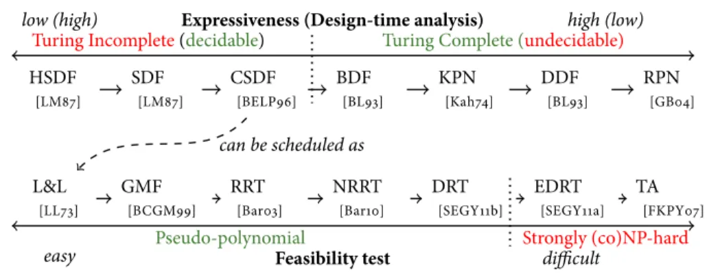
Several algorithms from the classical hard real-time multiprocessor scheduling theory [DB11] can performfast admission and scheduling decisions for incoming programs while providing hard real-time guarantees. Moreover, these algorithms enforce temporal isolation between running programs. Another key advantage of using classical hard real-time scheduling algorithms is the ability to derive in an analytical and fast way the minimum number of processors needed to schedule a set of tasks and the mapping of tasks to processors. Hard real-time scheduling theory and algorithms work in a similar way to model-based design; they abstract the programs in the form of areal-time task model. Such task models impose restrictions on the timing of the program tasks. As a result, it becomes easier to perform timing analysis of the program and reason about its behavior during the design phase. Several real-time task models have been proposed in the literature which differ in the complexity of theirfeasibility testsas shown in Figure 1.4. A feasibility test deals with the problem of deciding whether a given set of tasks can be scheduled to meet all their deadlines.
The most famous model is thereal-time periodictask model proposed by Liu and Layland in 1973 [LL73]–often called Liu and Layland (L&L) model. This model has simple feasibility analysis which led to its wide adoption. However, this model places several restrictions on the tasks such as:
• The releases (i.e., invocations) of all tasks are periodic, with constant interval between releases.
10 Chapter 1. Introduction
initiation or completion of releases of other tasks. • Execution time of each task is constant.
Several models were proposed to extend Liu and Layland model as shown in Figure 1.4. However, these extended models have more sophisticated feasibility analysis.
1.2
Problem Statement
We can summarize the discussion in Section 1.1 as follows. Model-based design and electronic system-level synthesis have emerged as de facto solutions to the problems of designing parallel software for MPSoCs and generating the complete MPSoC, re-spectively. However, no such de facto solution exists yet for the problem of scheduling parallel streaming programs on MPSoCs used in hard real-time systems. Scheduling has a direct influence on the architecture and mapping specifications needed to perform electronic system-level synthesis as shown in Figure 1.3. One possible and attractive solution is to use classical hard real-time scheduling algorithms due to their benefits mentioned in Section 1.1.3. However, most hard real-time scheduling algorithms as-sumeindependentperiodic or sporadic tasks [DB11]. Such a simple task model is not directly applicable to modern streaming programs which, as mentioned in Section 1.1.1, are typically modeled as directed graphs, where graph nodes represent actors (i.e., tasks) and graph edges represent data-dependencies. The actors in such graphs havedata-dependency constraintsand do not necessarily conform to the periodic or sporadic task models. Therefore, the core problem addressed by this dissertation is toinvestigate the applicability of hard real-time scheduling theory for real-time periodic tasks to streaming programs modeled as acyclic Cyclo-Static Dataflow (CSDF, [BELP96]) graphs.
1.3. Research Contributions 11 HSDF [LM87] SDF [LM87] CSDF [BELP96] BDF [BL93] KPN [Kah74] DDF [BL93] RPN [GB04] L&L [LL73] GMF [BCGM99] RRT [Bar03] NRRT [Bar10] DRT [SEGY11b] EDRT [SEGY11a] TA [FKPY07]
can be scheduled as
Expressiveness (Design-time analysis)
low (high) high (low)
Turing Complete (undecidable) Turing Incomplete(decidable)
Feasibility test
easy Pseudo-polynomial Strongly (co)NP-harddifficult
Figure 1.5:Bridging dataflow MoCs and real-time task models through the proposed scheduling
framework. The link indicates that any acyclic CSDF can be scheduled as a set of L&L tasks.
1.3
Research Contributions
The research contributions of this dissertation can be summarized as follows.
Contribution 1: Proposing a Scheduling Framework that Bridges Data-flow MoCs and Real-Time Task Models
12 Chapter 1. Introduction
CSDF annotated with WCET CSDF annotated with WCET
Scheduling Framework
Constraints by Designer CSDF annotated with WCET
Architecture Specifications
Mapping Specifications Temporal
Specifications
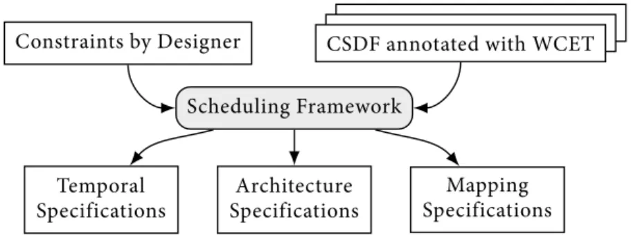
Figure 1.6:Input and outputs of the proposed scheduling framework
(i) type of scheduling algorithm, (ii) type of allocation algorithm, and (iii) values of parameters used to control the derivation of periods and deadlines as explained later in Chapter 4. The outputs of the framework are: (i) architecture specifications which describe how many processors are needed to schedule the programs, (ii) mapping specifications which associate each task with the processor on which it runs, and (iii) temporal specifications which consist of the parameters (i.e., periods, start times, and deadlines) of the periodic tasks corresponding to the CSDF actors together with the buffer sizes of the CSDF communication channels.
Additionally, the proposed scheduling framework establishes the following results: • Matched I/O rates graphs (which correspond to roughly 90% of streaming prog-rams) have a throughput under periodic schedules that is equal to their through-put under worst-case self-timed schedules. Periodic schedules here refers to scheduling the graph actors as real-time periodic tasks. This result opens the door for applying periodic scheduling to streaming programs.
• For certain classes of CSDF graphs, it is possible to achieve throughput and latency, under periodic schedules, that are equal to the throughput and latency under worst-case self-timed schedules. It is also shown that, for CSDF graphs in general, the latency can be reduced via reducing the deadlines of the actors along the critical paths.
Contribution 2: Proposing and Realizing a System-Level Design Flow that Incorporates the Proposed Scheduling Framework
1.4. Related Work 13
based on an existing state-of-the-art system-level design flow for streaming programs called Daedalus [TNS+07, NTS+08]. Similar to Daedalus, the proposed design flow starts from the sequential specifications of the programs, and then, generates in a fully automated manner the final system implementation, which provably meets the timing requirements of the programs. A complete implementation of the proposed design flow is available for download as an open source framework from http://daedalus.liacs.nl/. This implementation of the proposed design flow is called the DaedalusRTdesign flow. The proposed design flow is illustrated in Figure 1.7. It consists, in total, of six steps that are marked inside circles in Figure 1.7.Step 1accepts, as input, a set of SANLPs and then uses thePNgencompiler to parallelize them and generate the parallel specification of these input programs. The parallel specification consists of the Polyhedral Process Network (PPN, [VNS07]) representation of the program. PPN is a parallel MoC that is useful for code generation and optimizations. However, it is not suitable for analytical performance analysis. This leads us to the next step.
InStep 2, the generated PPNs in step 1 are used to construct the performance analysis model, i.e., CSDF model. Given a PPN, we use the algorithm proposed in [BZNS12] to derive a CSDF graph that is equivalent to the given PPN.
InStep 3, we perform WCET analysis on the parallel specification of the program. WCET analysis, as mentioned earlier, can be performed through either static analysis tools or profiling the code on the target MPSoC platform.
InStep 4, the CSDF models generated in step 2, the WCET values generated in step 3, and the user constraints, which include for example the type of scheduler and other parameters as explained earlier, are fed to the proposed scheduling framework explained in Contribution 1. This results in: (i) the architecture specification, which describes how many processors are needed to schedule the programs, and (ii) the mapping specification, which describes the allocation of tasks to processors.
InStep 5, the PPNs together with architecture and mapping specifications are pro-cessed by ESPAM [NSD08]. ESPAM is an ESL synthesis tool that supports MPSoC synthesis from PPNs. We have extended ESPAM to support synthesizing the target MPSoC hardware and software. The output from this step is a full MPSoC implementa-tion consisting of the RTL needed to perform low-level synthesis for FPGA or ASIC together with the software running on each processor in the MPSoC.
Step 6 is the last step in the design flow and consists of performing low-level synthesis for FPGA or ASIC together with compiling the code for each processor.
1.4
Related Work
14 Chapter 1. Introduction
SANLP
Polyhedral Process Network
CSDF Model SANLP
Polyhedral Process Network
CSDF Model Constraints by Designer SANLP
Automated Parallelization (PNgencompiler)
Polyhedral Process Network
Model Construction WCET Analysis
WCET Values CSDF Model Scheduling Framework Architecture Specifications Mapping Specifications Temporal Specifications System-Level Synthesis (ESPAM)
RTL + Software
Synthesis/Compilation
MPSoC Implementation (for ASIC or FPGA)
System Deployment 1 ○ 3 ○ 2 ○ 4 ○ 4 ○ 4 ○ 5 ○ 5 ○ 5 ○ 6 ○ 7 ○ provably satisfied D e si g n T im e Tape-out R u n T im e
Figure 1.7:Overview of the proposed design flow
this dissertation. The related work is organized into two categories: hard real-time scheduling of streaming programs, and design flows for hard real-time streaming systems.
1.4.1 Hard Real-Time Scheduling of Streaming Programs
1.4. Related Work 15
Several scheduling techniques (e.g., [Mor12]) utilize this property by converting a given SDF/CSDF into an HSDF graph and then performing the scheduling analysis on the HSDF. However, the resulting HSDF graph has a size that grows exponentially with the size of the input SDF/CSDF. Therefore, such scheduling techniques have two disadvantages. First, the resulting HSDF might be huge which introduces large overhead when the actual HSDF is scheduled on the system. Second, in a periodic schedule of CSDF, each actor must have a start time and a period and each channel must have a buffer size. By deriving the schedule for the HSDF graph, it is possible to derive a start time and a period for each CSDF actor. However, it is not clear how to derive a buffer size for each CSDF channel from the buffer sizes of the HSDF.
Parks and Lee [PL95] studied the applicability of non-preemptive fixed task priority scheduling with rate monotonic priority assignment to streaming programs modeled as SDF graphs. Our work differs in the following aspects. First, they considered non-preemptive scheduling, while we consider only preemptive scheduling. Non-preemptive scheduling is known to be NP-hard in the strong sense even for the unipro-cessor case [JSM91]. Second, they considered SDF graphs which are a subset of the more general CSDF graphs.
Verhaegh et al. [VLA+96] proposed Multidimensional Periodic Scheduling (MPS) to schedule digital signal processing programs written as a set of nested loops and modeled using Signal Flow Graphs (SFG). The inputs to MPS are the SFG and a set of explicit timing constraints. Given an SFG, MPS derives a schedule for each operation, where this schedule is described by multiple periods and offsets, and a buffer size for each channel such that the precedence and timing constraints are met. The scheduled operations execute in a strictly periodic manner (similar to the real-time periodic model). Verhaegh et al. showed that MPS is NP-hard and they proposed a two-stage solution approach in [VAvGL01]. The MPS framework is very similar to the framework proposed in Chapter 4 in that both frameworks derive the periods and start times of the tasks and the buffer sizes of the channels. However, the frameworks differ in the considered MoC. MPS considers SFG, while the framework in Chapter 4 considers CSDF which is more general than SFG [PC13]. Another difference is that the framework in Chapter 4 can derive a deadline for each task to reduce the graph latency.
16 Chapter 1. Introduction
or equal to the consumption threshold. In contrast, CSDF supports a sequence of pre-defined production/consumption rates. As a result, the analysis technique in [God98] is not applicable to CSDF graphs.
Ziegenbein et al. [ZUE00] proposed a technique to optimize the response time of SDF graphs under Earliest Deadline First (EDF) scheduling assuming jittery input streams. Their technique accepts, as input, the SDF graphs, the average period of each actor, and the jitter bounds of the input streams. Then, they revise the deadline of each actor in such a way that the data dependencies are respected and the total response time is minimized. Our approach differs from [ZUE00] in the following aspects. First, we compute all the scheduling parameters of the tasks including the deadline, while in [ZUE00] the authors assume that the periods are given. Thus, our approach gives the designer greater flexibility in controlling the timing behavior of the tasks. Second, we consider CSDF graphs which extend the SDF model considered in [ZUE00].
Bekooij et al. [BHM+05] analyzed the impact of TDM scheduling on programs mod-eled as SDF graphs running on embedded real-time multiprocessor systems. Wiggers et al. [WBS09] proposed a classification scheme for run-time scheduling algorithms based on the causes of interference among programs. They identified two causes of interference which are (i) how often other tasks are executed and (ii) what execution time is associated with these executions. According to Wiggers taxonomy [WBS09], run-time scheduling algorithms are classified into:
1. Non-starvation-freealgorithms: under such algorithms, interference depends on (i) and (ii). Examples include fixed-task priority scheduling.
2. Starvation-freealgorithms: interference is independent of (i) but depends on (ii). Examples include round-robin scheduling.
3. Budget-schedulers: interference is independent of (i) and (ii). Thus, a budget scheduler guarantees every task a minimum amount of timexin every time interval of lengthy. Examples of budget schedulers include TDM and Constant Bandwidth Server (CBS, [AB98]).
Wiggers et al. defined a subset of dataflow graphs calledfunctionally deterministic dataflow graphsand showed that such graphs have time deterministic behavior under budget schedulers. CSDF is an example of a functionally deterministic dataflow graph. In [SBW09], Steine et al. proposed a priority-based budget scheduling algorithm that overcomes some of the limitations of TDM. Recently, Hausmans et al. [HWGB13] extended the analysis in [BHM+05, WBS09] to programs modeled as arbitrary HSDF graphs when they are scheduled using algorithms of the first class according to Wiggers taxonomy. In another work, Hausmans et al. [HGWB13] proposed a two parameter
(σ,ρ)workload characterization to reduce the gap between the worst-case throughput
determined by the analysis and the actual throughput of the program. The(σ,ρ)
1.4. Related Work 17
task to provide throughput and latency guarantees. Compared to [BHM+05, HWGB13], the framework in Chapter 4 applies the analysis directly to a more expressive MoC (namely CSDF) and avoids the conversion to a larger HSDF. Compared to [WBS09, SBW09], we use the real-time periodic model which does not restrict the designer to a certain class of algorithms as defined by Wiggers taxonomy. The designer can use any algorithm that supports the underlying task model. Compared to [HGWB13], we consider “classical” hard real-time tasks, where each execution of a task must meet its deadline. In contrast, under the(σ,ρ)workload characterization, the average WCET
is used to improve the minimum guaranteed throughput/latency. Thus, an internal task in the dataflow graph may miss its deadline without causing the program to violate its guaranteed throughput/latency.
Thiele and Stoimenov [TS09] proposed an analysis framework for HSDF graphs based on Real-Time Calculus (RTC, [CKT03]). Their analysis framework provides upper and lower bounds on the performance metrics under different scheduling policies (e.g., TDM and fixed task priority scheduling). An advantage of their framework is its ability to handle cyclic graphs. However, their framework acts as a general performance analysis technique that provides only upper and lower bounds on the performance. In contrast, our scheduling framework computes the tasks’ parameters that guarantee a certain performance under certain scheduling policies. Moreover, we apply the analysis directly on the more general CSDF model (although acyclic graphs only), while the framework in [TS09] applies the analysis to HSDF graphs. This means that a program modeled as an SDF/CSDF graph must be converted into HSDF in order to apply the analysis in [TS09]. Such conversion has disadvantages as mentioned earlier.
Moreira [Mor12] has investigated temporal analysis of hard real-time radio prog-rams modeled as SDF graphs. He proposed a scheduling framework based on TDM combined with static allocation. He also proved that it is possible to derive a periodic schedule for the actors of a cyclic SDF graph if and only if the periods are greater than or equal to the maximum cycle mean of the graph. He formulated the conditions on the start times of the actors in the equivalent HSDF graph in order to enforce a periodic execution of every actor as a Linear Programming (LP) problem. Our approach differs from [Mor12] in the following aspects. First, we use the periodic task model which allows applying a variety of hard real-time scheduling algorithms for multiprocessors. Second, we use the CSDF model which is more expressive than the SDF model and perform the analysis directly on CSDF instead of converting it into HSDF as done in [Mor12].
18 Chapter 1. Introduction
the maximum throughput for a given SDF program. WhenKi = 1 for all tasks, we
obtain 1-periodic schedules which are equivalent to the schedules generated using the real-time periodic task model. Thus,K-periodic schedules serve as a powerful tool to analyze different scheduling policies. However, the realization of such schedules is more complex than the 1-periodic ones. In this dissertation, we prove the existence of 1-periodic schedules for acyclic CSDF graphs. 1-periodic schedules are easier to realize, however, this simplicity comes at the price of extra buffer requirements as shown later in Chapter 6.
Bouakaz et al. [BTV12, BT13] proposed recently a new dataflow model calledAffine Dataflow (ADF)which extends the CSDF model. They proposed as well an analysis framework similar to ours to schedule the actors in an ADF graph as periodic tasks. They claim also that their analysis framework is capable of handling cyclic ADF graphs. An advantage of their approach is the enhanced expressiveness of the ADF model. The framework proposed in [BTV12, BT13] has been proposed after our framework and the authors in [BTV12, BT13] refer to our framework and compare empirically their framework with ours using the benchmarks explained later in Chapter 6. For most benchmarks, both CSDF and ADF achieve the same throughput and latency while requiring the same buffer sizes. However, in few cases, ADF results in reduced buffer sizes compared to CSDF [BT13].
Benabid-Najjar et al. [BNHMMK12] studied periodic scheduling of SDF graphs. For acyclic graphs, they proved that any acyclic SDF graph can be scheduled as a set of periodic tasks. For cyclic SDF graphs, they showed that the existence of a periodic schedule depends on the number of initial tokens in the graph cycles and provided a framework to derive the graph throughput under a periodic schedule. Compared to [BNHMMK12], our framework proves the existence of periodic schedules for acyclic CSDF graphs, which are more expressive than SDF graphs. Recently, Bodin et al. [BMKdD13] extended the work in [BNHMMK12] to cyclic CSDF graphs by providing a framework to derive the maximum throughput of a CSDF graph under a periodic schedule. Similar to [BT13], the work in [BMKdD13] is very recent and was proposed after our framework.
1.4. Related Work 19
with the real-time periodic task model. Using the real-time periodic task model has the following advantages. First, any scheduling algorithm that supports the real-time periodic task model can be used to schedule the programs. Second, multiple programs can be scheduled, while preserving temporal isolation, as long as the programs’ tasks conform to the task model and satisfy the schedulability test of the used scheduling algorithm. Third, the minimum number of processors needed to schedule the programs can be determined in a fast and analytical way.
1.4.2 Design Flows for Hard Real-Time Streaming Systems
Several design flows for automated mapping of streaming programs onto MPSoC platforms are surveyed in [GHP+09]. Most of these flows deal with soft real-time streaming systems. Additionally, these flows assume that the program model is derived manually by the designer/programmer. In contrast, our proposed design flow deals with hard real-time systems and derives the program model in a completely automated manner.
Distributed Operation Layer (DOL, [TBHH07]) is a framework for mapping parallel applications onto tiled MPSoCs. It accepts, as input, an application, which is specified as a process network, and an architecture specification. After that, it uses multi-objective optimization algorithms to perform the mapping of application to architecture. Then, it applies analytical performance analysis based on Real-Time Calculus (RTC, [CKT03]) to estimate the performance of the application after mapping. Our proposed design flow differs from DOL in the following aspects. First, we perform automated parallelization and model construction of the input applications, while DOL assumes that the input is a parallel application. Second, Real-Time Calculus gives worst-case upper and lower bounds on the performance, however, in reality these bounds may be rarely reached. In contrast, our proposed design flow guarantees a certain performance of the programs under certain scheduling policies.
PeaCE [HKL+08] is an integrated hardware/software co-design framework for embedded multimedia systems. It employs Synchronous Piggybacked Dataflow (SPDF) for computation tasks and Flexible Finite State Machines (fFSM) for control tasks. PeaCE uses hardware/software co-simulations during the design phase in order to meet certain timing constraints. In contrast, our proposed flow avoids these iterative steps by applying hard real-time multiprocessor scheduling theory to guarantee temporal isolation and a given throughput of each application running on the target MPSoC.
20 Chapter 1. Introduction
case [JSM91]. Moreover, we consider a more expressive MoC, namely the CSDF model.
CompSOC [GAC+13] is a platform and an associated design flow for running applications modeled as CSDF graphs. The platform part (called CoMPSoC [HGBH09]) provides predictability andcomposability, which means that the applications running on the system are completely isolated in terms of execution time, power, and access to shared resources. Similar to CoMPSoC, the hardware architecture proposed in Chapter 5 is designed to provide predictability. For the software side, CompSOC uses a custom OS called Compose that implements two-level hierarchical scheduling. In the first (or base) level, it divides the processor time into fixed intervals and uses TDM scheduling to provide complete isolation between the applications running on different intervals. In the second level, each interval may use a different scheduling policy (e.g., EDF or round-robin) to schedule the tasks executed within the interval. The associated design flow with CompSOC accepts, as input, the CSDF models of the application. Then, it uses SDF3[SGB06] to derive the buffer sizes and TDM interval sizes needed to guarantee a certain performance. Therefore, CompSOC provides a platform for executing given parallel applications, while our proposed design flow is concerned with providing a complete integrated design flow that parallelizes the applications and then derives the scheduling and platform parameters that guarantee a certain performance.
MAPS [Cas13] is a design flow for mapping dataflow applications onto MPSoCs. The design flow accepts, as input, a set of sequential programs written in a variant of C called C for Process Networks (CPN). After that, it parallelizes these programs and generates a performance analysis model based on Kahn Process Networks (KPN, [Kah74]). Then, it uses a simulation-based composability analysis to provide certain performance guarantees on the target platform. Our proposed design flow differs from MAPS in that our flow provides hard real-time guarantees to the programs, while MAPS provides soft real-time guarantees.
1.5. Organization of this Dissertation 21
1.5
Organization of this Dissertation
The rest of this dissertation is organized as follows:
1. Chapter 2 presents an overview of dataflow models and hard real-time schedul-ing theory. This overview is necessary to understand the subsequent chapters. 2. Chapter 3 presents the first two stages in the proposed design flow: automated
parallelization and model construction.
3. Chapter 4 presents the key contribution of this dissertation: scheduling frame-work for streaming programs. This frameframe-work constitutes the third stage in the proposed design flow.
4. Chapter 5 presents the fourth stage of the proposed design flow (i.e., ESL syn-thesis) and explains the hardware and software parts of the synthesized systems. 5. Chapter 6 presents the results of empirical evaluation of the proposed scheduling
framework and design flow. This empirical evaluation is performed through a set of experiments.
Chapter 2
Background
Essentially, all models are wrong, but some are useful.
George E. P. Box
T
HIS chapter introduces the notations, definitions, and existing results that are used in the subsequent chapters. It also contains material from the theory of dataflow models and hard real-time scheduling that is needed to understand the subsequent chapters.2.1
Notations
We present in Table 2.1 a summary of the mathematical notations used throughout this dissertation.
Definition 2.1.1(Partition of a Set). LetVbe a set. Anx-partition ofVis a set, denoted byxV, where
xV= {xV
1,xV2,⋯,xVx},
such that each subsetxVi ⊆V, and
x ⋂ i=1
xV
i = ∅and x ⋃ i=1
xV i =V
2.2
Parallel Execution of Programs
24 Chapter 2. Background
Table 2.1:Summary of mathematical notations
Symbol Meaning
N The set of natural numbers excluding zero
N0 N∪ {0}
Z The set of integers
Q The set of rational numbers
⋃︀x⋃︀ The cardinality (i.e., size) of a setx ˆ
x The maximum value ofx ˇ
x The minimum value ofx
lcm The least common multiple operator gcd The greatest common divisor operator
÷ The integer division operator mod The integer modulo operator
xV Anx-partition of a setV(see Definition 2.1.1)
Definition 2.2.1(Program). Aprogram(also calledapplication) is a sequence of operations (also called statements) that transform a given input to an output.
A statement can be a simple expression (e.g.,z = x + y), an invocation of a function (e.g.,z = f(x,y)), or a control statement (e.g., if(x>1)). For some programs, the statements need to be executed in a strictly sequential way in order to maintain the correct functionality of the program. For some other programs, the statements can be executed in a parallel fashion while maintaining the correct func-tionality. In general, the main objective of executing the statements of a given program in parallel is to achieve aspeedup. Let ∆1be the time needed to run the program on one processor, and ∆mbe the time needed to run the program onmprocessors. We define the speedup as:
speedup= ∆1
∆m (2.1)
An ideal parallel implementation of a program running onmprocessors achieves a speedup equal tom. However, Amdahl in 1967 [Amd67] observed that, in reality, any program consists of two portions: aparallelizableportion, and asequentialportion. The statements in the sequential portioncan notbe executed in parallel, and hence, do not benefit from execution on multiprocessor systems. Letf ∈ (︀0, 1⌋︀be a fraction that
denotes the relative size of the parallelizable portion of a program. Amdahl showed that the actual speedup is given by:
speedup= 1 (1−f) + f
m
2.2. Parallel Execution of Programs 25
For example, for a program where f =0.9 (i.e., 90% of the program is parallelizable),
the maximum speedup is:
maximum speedup= lim m→∞
1
(1−0.9) + 0.9 m
= 1
0.1 =10 (2.3)
This means that the maximum speedup that can be obtained by executing the program on a multiprocessor system is 10. Therefore, executing this program on more than 10 processors does not result in an extra speedup.
The ability to execute two program statements in parallel is constrained by thedata dependenciesbetween them. For example, if a statementSjrequires the data produced by statementSi, thenSjmust be executed afterSi has completed its execution. To find all data dependencies in a given program, one needs to performdependency analysis. Dependency analysis reveals, for a given program, all data dependencies among the statements of the program. LetSbe a program whereSiandSjrepresent two statements of the program. Additionally, let i n p u t(Si)be the set of resources1
read bySi, and ou t p u t(Si)be the set of resources written to bySi. We denote the
sequential execution ofSjafterSibySi→Sj, while we denote the parallel execution
ofSi andSj bySi ∥ Sj. Bernstein [Ber66] showed thatSi → Sj andSi ∥ Sj are
equivalent provided that:
1. ou t p u t(Si) ∩ou t p u t(Sj) = ∅
2. ou t p u t(Si) ∩i n p u t(Sj) = ∅
3. ou t p u t(Sj) ∩i n p u t(Si) = ∅
The three conditions above are known in the literature asBernstein’s conditions. They form the basis of how we can analyze a given program to determine the statements that can be executed in parallel. During the execution of a programS, we say that a statementSi precedesa statementSj, denoted bySi ≺Sj, ifSi is executed beforeSj.
Given a programSwhereSiandSjare two statements andSi ≺Sj, one can identify
the following types of data dependencies:
• Flow (True) Dependence: If ou t p u t(Si) ∩i n p u t(Sj) ≠ ∅
• Anti-Dependence: If i n p u t(Si) ∩ou t p u t(Sj) ≠ ∅
• Output Dependence: If ou t p u t(Si) ∩ou t p u t(Sj) ≠ ∅
• Input Dependence: If i n p u t(Si) ∩i n p u t(Sj) ≠ ∅
Standard dataflow analysis [ALSU86] is a body of techniques that derive the data dependencies among the statements of a given program. Array dataflow analysis [Fea91] is a technique which performs dataflow analysis for SANLP programs. Feautrier [Fea91] showed that array dataflow analysis can be used to construct aparallelversion of a given SANLP program. This means that programs written in SANLP form can be
26 Chapter 2. Background
automaticallyanalyzed and parallelized. An example of a tool which implements such automated analysis and parallelization is thePNgencompiler [VNS07]. The details of how a parallel program is derived using automated parallelization are explained in Chapter 3.
2.3
Cyclo-Static Dataflow (CSDF)
As mentioned earlier in Chapter 1, we use in this dissertation the Cyclo-Static Dataflow (CSDF) model for modeling streaming programs. In this section, we introduce this model and its properties.
CSDF is a dataflow model that extends the well-known Synchronous Dataflow (SDF, [LM87]) model. It is defined in [BELP96] as a directed graphG = (A,E),
whereAis a set of actorsthat correspond to the graph nodes andE ⊆A×Ais a set
of communication channelsthat correspond to the graph edges. Actors represent statements in the program that transform incoming data streams into outgoing data streams, while communication channels represent data dependencies among the actors. The communication channels carry streams of data, and an atomic data object is called atoken. A channelEu ∈Eis a first-in, first-out (FIFO) queue with unbounded capacity
defined by a tupleEu = (Ai,Aj). The tuple means thatEuis directed fromAi(called source) toAj(calleddestination). An actor receiving an input stream of the program is calledinput actor, and an actor producing an output stream of the program is called output actor. ApathWkbetween actorsAaandAzis an ordered sequence of channels defined asWk= {(Aa,Ab),(Ab,Ac),⋯,(Ay,Az)}. A pathWkis calledoutput pathif
the starting actorAais an input actor and the ending actorAzis an output actor. For a graphG, we useWto denote the set of all output paths inG. Each actorAi ∈Ais
associated with two sets of channels and two sets of actors. The sets of channels are theinput channels set, denoted by inp(Ai), which consists of all the input channels to Ai, and theoutput channels set, denoted by out(Ai), which consists of all the output
channels fromAi. The sets of actors are thesuccessors set, denoted by succ(Ai), and
thepredecessors set, denoted by prec(Ai). They are given by:
succ(Ai) = {Aj∈A∶ ∃Eu= (Ai,Aj) ∈E} (2.4)
prec(Ai) = {Aj∈A∶ ∃Eu = (Aj,Ai) ∈E} (2.5)
We assume that: (1) for any input actorAi, prec(Ai) = ∅, and (2) for any output actor Aj, succ(Aj) = ∅.
Every actorAj∈Ahas anexecution sequence(︀fj(1), fj(2),⋯, fj(𝒩j)⌋︀of length 𝒩j. The interpretation of this sequence is: thenth time that actorAjis fired, it
ex-ecutes the code of function fj(((n−1)mod𝒩j) +1). Similarly, production and
2.3. Cyclo-Static Dataflow (CSDF) 27
Algorithm 1L ev e l s(G)
Require: Acyclic CSDF graphG= (A,E)
1: i←1
2: whileA≠ ∅do
3: LA
i← {Aj∈A∶prec(Aj) = ∅}
4: E′i← {Eu∈E∶ ∃Ak∈LAisuch thatEu= (Ak,Al)}
5: A←A∖LAi
6: E←E∖E′i
7: i←i+1
8: end while
9: L←i−1
10: return L-partition ofAgiven byLA= {LA1,LA2,⋯,LAL}.
production of actor Aj on channel Eu is represented as a sequence of constant in-tegers (︀xuj(1),xuj(2),⋯,xuj(𝒩j)⌋︀. Thenth time that actor Aj is fired, it produces xu
j(((n−1)mod𝒩j) +1)tokens on channelEu. The consumption of actorAk is
completely analogous; the token consumption of actorAkfrom a channelEu is rep-resented as a sequence(︀yuk(1),yuk(2),⋯,yuk(𝒩k)⌋︀. The firing rule of a CSDF actor Akis evaluated as “true” for itsnth firing if and only if all its input channels contain
at least yuk(((n−1)mod𝒩k) +1)tokens. The total number of tokens produced by
actorAjon channelEu during the firstninvocations is denoted byXuj(n)and given
byXuj(n) = ∑nl=1xuj(l). Similarly, the total number of tokens consumed by actorAk
from channelEu during the firstninvocations is denoted byYku(n)and given by Yu
k(n) = ∑nl=1yuk(l).
An acyclic CSDF graph has anumber of levels, denoted byL, and is given by
Algorithm 1. Algorithm 1 builds anL-partition ofA, denoted byLA, by partitioning it
in a way similar totopological sort. The actors belonging to subsetLA
i are said to be level-i actors.
An important property of the CSDF model is itsdecidability, which is, as mentioned in Chapter 1, the ability to derive at compile-time a schedule for the actors. This is formulated in Definition 2.3.1 and Theorem 2.3.1.
Definition 2.3.1(Valid Static Schedule [BELP96]). Given a connected CSDF graph G, avalid static scheduleforGis a finite sequence of actors invocations that can be repeated infinitely on the incoming sample stream while the amount of data in the buffers remains bounded. A vectorq⃗= (︀q1,q2,⋯,q⋃︀A⋃︀⌋︀T, whereqj>0, is arepetition
vectorofGif eachqjrepresents the number of invocations of an actorAjin a valid static schedule forG. The repetition vector ofGwith the smallest norm is called thebasic repetition vectorofGand is denoted byq⃗ˇ.Gisconsistentif there exists a repetition
28 Chapter 2. Background
and liveness are required for the existence of a valid static schedule.
Bilsen et al. [BELP96] proved the following theorem:
Theorem 2.3.1. Let G be a CSDF graph. A repetition vectorq⃗= (︀q1,q2,⋯,q⋃︀A⋃︀⌋︀Tof G is given by
⃗
q=Θ⋅ ⃗r, with Θjk= )︀ ⌉︀ ⌉︀ ⌋︀ ⌉︀ ⌉︀ ]︀
𝒩j if j=k
0 otherwise (2.6)
where⃗r= (︀r1,r2,⋯,r⋃︀A⋃︀⌋︀Tis a positive integer solution of the balance equation
Γ⋅ ⃗r= ⃗0 (2.7)
and where thetopology matrix Γ∈Z⋃︀E⋃︀×⋃︀A⋃︀is defined by
Γuj= )︀ ⌉︀ ⌉︀ ⌉︀ ⌉︀ ⌉︀ ⌋︀ ⌉︀ ⌉︀ ⌉︀ ⌉︀ ⌉︀ ]︀
Xuj(𝒩j) if actor Ajproduces on channel Eu −Yju(𝒩j) if actor Ajconsumes from channel Eu
0 Otherwise.
(2.8)
Definition 2.3.2. For a consistent and live CSDF graphG, anactor iterationis the invocation of an actorAi∈Aforqitimes, and agraph iterationis the invocation of everyactorAi ∈Aforqi times, whereqi∈ ⃗q.
Corollary 2.3.1(From [BELP96]). If a consistent and live CSDF graph G completes k iterations, where k∈N, then the net change to the number of tokens in the buffers of G is zero.
Lemma 2.3.1. Any acyclic consistent CSDF graph is live.
Proof. Bilsen et al. proved in [BELP96] that a CSDF graph is live if and only if every cycle in the graph is live. Equivalently, a CSDF graph deadlocks only if it contains at least one cycle. Thus, absence of cycles in a CSDF graph implies its liveness. ∎
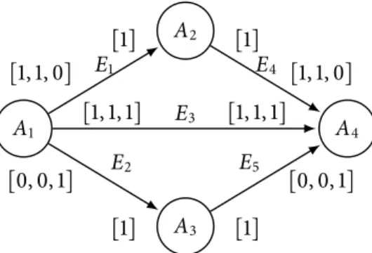
2.4. Real-Time Scheduling 29 A1 A2 A3 A4 E1 E2 E3 E4 E5
(︀1, 1, 0⌋︀
(︀0, 0, 1⌋︀ (︀1, 1, 1⌋︀
(︀1⌋︀ (︀1⌋︀
(︀1⌋︀ (︀1⌋︀
(︀1, 1, 0⌋︀
(︀0, 0, 1⌋︀ (︀1, 1, 1⌋︀
Figure 2.1:Example of a CSDF graph that corresponds to the SANLP program in Listing 1
byW={W1= {(A1,A2),(A2,A4)},W2= {(A1,A3),(A3,A4)},W3 = {(A1,A4)}}.
Based on Theorem 2.3.1 on page 28, we compute the basic repetition vector as follows:
Γ= ⎨ ⎝ ⎝ ⎝ ⎝ ⎝ ⎝ ⎝ ⎝ ⎝ ⎪
2 −1 0 0
1 0 −1 0
3 0 0 −3
0 1 0 −2
0 0 1 −1
⎬ ⎠ ⎠ ⎠ ⎠ ⎠ ⎠ ⎠ ⎠ ⎠ ⎮
,⃗r= ⎨ ⎝ ⎝ ⎝ ⎝ ⎝ ⎝ ⎝ ⎪ 1 2 1 1 ⎬ ⎠ ⎠ ⎠ ⎠ ⎠ ⎠ ⎠ ⎮
, Θ= ⎨ ⎝ ⎝ ⎝ ⎝ ⎝ ⎝ ⎝ ⎪
3 0 0 0
0 1 0 0
0 0 1 0
0 0 0 3
⎬ ⎠ ⎠ ⎠ ⎠ ⎠ ⎠ ⎠ ⎮
, andq⃗ˇ= ⎨ ⎝ ⎝ ⎝ ⎝ ⎝ ⎝ ⎝ ⎪ 3 2 1 3 ⎬ ⎠ ⎠ ⎠ ⎠ ⎠ ⎠ ⎠ ⎮
We show later in Chapter 3 how such a graph can be automatically derived from a given
SANLP program. ◻
2.4
Real-Time Scheduling
In this section, we introduce the time periodic task model, some important real-time scheduling concepts, and schedulability analysis for uniprocessor and multipro-cessor systems.
2.4.1 Task Model
A system is composed of a set ofmidentical processors{π1,π2,⋯,πm}. These
pro-cessors execute a set ofntasksT= {T1,T2,⋯,Tn}and a taskTimay be preempted at
any time. A taskTicorresponds to a CSDF actorAiand we model the tasks using the real-time periodictask model. Under the periodic task model, each task is arecurrent one with a constant inter-arrival time. AtaskTi ∈Tis characterized by a 4-tuple of
integersTi = (Si,Ci,Pi,Di). The tuple parameters are interpreted as follows: Si ≥0
is thestart timeofTi in absolute time units,Ci >0 is theWorst-Case Execution Time (WCET)ofTi,Pi≥Ciis thetask period(i.e., inter-arrival time) in relative time units,
30 Chapter 2. Background
A periodic taskTiis invoked at time instantsri,k=Si+kPifor allk∈N0. When Ti is invoked, we say thatTireleasesajob. Thekth job (or invocation) ofTiis denoted
byTi,k. Upon invocation, a task must execute forCi time-units. ThedeadlineDi is interpreted as follows: jobTi,khas to finish its execution before timedi,k=ri,k+Difor
allk∈N0. IfDi =Pi, thenTi is said to have animplicit-deadline. IfDi<Pi, thenTiis
said to have aconstrained-deadline. If all the tasks in a tasksetTare implicit-deadline tasks, then we say thatTis animplicit-deadline taskset. Otherwise, we say thatTis a constrained-deadline taskset. Similarly, if all the tasks in a tasksetThave the same start time, then we say thatTissynchronous. Otherwise, we say thatTisasynchronous. For synchronous tasksets, we assume that their start time is 0.
Theutilizationof a taskTi isui =Ci⇑Pi. For a tasksetT, the total utilization ofT
isusum(T) = ∑Ti∈Tuiand the maximum utilization factor ofTis ˆu(T) =maxTi∈Tui.
Similarly, thedensity of a taskTi isδi = Ci⇑min(Di,Pi), the total density ofT is δsum(T) = ∑Ti∈Tδi, and the maximum density ofTis ˆδ(T) =maxTi∈Tδi. Note that
the density is equivalent to the utilization for implicit-deadline tasks.
Theprocessor demand, denoted by demand(Ti,t1,t2), of a task Ti over a time
interval(︀t1,t2⌋︀is the total computation time of all the jobs ofTi having activation time
and deadline within(︀t1,t2⌋︀. According to [BRH90], demand(Ti,t1,t2)is given by:
demand(Ti,t1,t2) =ζ(Ti,t1,t2) ⋅Ci (2.9)
whereζ(Ti,t1,t2)is the total number ofTijobs that are activated in the interval(︀t1,t2⌋︀
and have a deadline within the interval(︀t1,t2⌋︀. The authors in [BRH90] showed that ζ(Ti,t1,t2)is given by:
ζ(Ti,t1,t2) =max{0,⃒t2−Si−Di
Pi )︁ −max{0,⌊︂
t1−Si
Pi }︂} +1} (2.10)
For a tasksetT, the processor demand ofTover the time interval(︀t1,t2⌋︀is denoted
by demand(T,t1,t2)and given by:
demand(T,t1,t2) = ∑ Ti∈T
demand(Ti,t1,t2) (2.11)
2.4.2 Scheduling Concepts
Given a system and a tasksetT, acorrect scheduleis one that allocates a processor to a taskTi ∈Tfor exactlyCitime units in the interval(︀Si+kPi,Si+kPi+Di)for allk∈N0,
2.4. Real-Time Scheduling 31
according to some criteria (e.g., minimizing energy). However, offline scheduling lacks the flexibility to deal with new events at run-time. In contrast, online scheduling can deal with such new events at run-time. However, online scheduling introduces extra overheads due to the scheduling decisions taken during run-time. In the rest of this dissertation, we assume online scheduling algorithms unless we explicitly mention otherwise.
According to [DB11], real-time multiprocessor scheduling algorithms can be viewed as attempting to solve two problems:
• Thepriority assignmentproblem: when and in what order with respect to other tasks, each job should execute.
• Theallocationproblem: on which processor a task should execute and whether a task can migrate between processors.
As a result, real-time multiprocessor scheduling algorithms can be classified based onpriorityas follows [DB11]:
• Fixed task priority: Each task has a single priority that is used for all its jobs. • Fixed job priority: The jobs of a single task may have different priorities, however,
each job has a single priority. An example of an algorithm using this policy is the Earliest Deadline First (EDF, [LL73]) algorithm.
• Dynamic priority: A single job might have different priorities during the course of its execution. An example is the Least Laxity First (LLF) algorithm.
Based onallocation, algorithms can be classified as follows [DB11]:
• No migration: Each task is allocated to a processor and no migration is permitted. • Task-level migration: The jobs of a task may execute on different processors,
however, a single job can only execute on a single processor.
• Job-level migration: A job may execute on more than one processor, however, it may not execute on more than one processor at the same time.
A scheduling algorithm that does not permit migration at all is said to be apartitioned scheduling algorithm, while an algorithm that permits all tasks to be migrated between all processors is said to be aglobalalgorithm, and finally an algorithm that permits a subset of tasks to be migrated among a subset of processors is said to be ahybrid algorithm.