i
SINGLE-MOLECULE FLUORESCENCE STUDIES OF DNA BENDING DURING PROKARYOTIC MISMATCH REPAIR INITIATION
Jacob Wayne Gauer
A dissertation submitted to the faculty at the University of North Carolina at Chapel Hill in partial fulfillment of the requirements for the degree of Doctor of Philosophy in the Department of Chemistry.
Chapel Hill 2015
iii ABSTRACT
Jacob Wayne Gauer: SINGLE-MOLECULE FLUORESCENCE STUDIES OF DNA BENDING DURING PROKARYOTIC MISMATCH REPAIR INITIATION
(Under the direction of Dorothy Erie)
DNA mismatch repair (MMR) is a process that is responsible for repairing base-base mismatches and insertion/deletion loop errors incorporated during DNA replication. In humans, deficiencies in MMR are linked to cancers, including Lynch Syndrome. MMR is initiated by MutS in prokaryotes (or the MutS homologs in eukaryotes), which is responsible for recognizing the error in the DNA. Upon error
recognition, MutS undergoes ATP-dependent conformational changes to form a sliding clamp state that moves along the length of the DNA. This state is thought to be important for downstream repair events, such as recruitment of the second protein in the pathway, MutL.
Recent single-molecule fluorescence studies have led to a refined model for error recognition and sliding clamp formation by Thermus aquaticus MutS. While it is well established that MutS bends DNA and that this DNA bending is dynamic in the absence of nucleotides, little evidence for the DNA bending status through MMR initiation exists in the presence of ATP.
In this work, the nucleotide dependence of Thermus aquaticus MutS-induced DNA bending throughout sliding clamp formation is characterized. The current model for MutS conformational changes is then modified to reflect the newfound DNA bending information. To this end, single-molecule
v
ACKNOWLEDGEMENTS
I did not want to do this. I never really saw myself earning a Ph.D. doing scientific research. Somehow, though, I have dragged, clawed, and whined my way through the last several years to make it here. I could not have done this alone, and I owe so many people for encouraging me, forcing me even, to stay the path and make it to the end.
I must start by recognizing my advisor, Dorothy. You have allowed me to define success in my own way, a trait that has been vital to perseverance. You have shown me that in a sea of never-ending disappointment and discouragement, nothing is ever as bad as it seems. At many times, I have been close to quitting, but you have always managed to pull me back from the edge to face the problems at hand. This thesis only exists because of your guidance. You are a wise, fervid, and, at times, weird mentor, and I aspire to become more like you.
To my husband, Aaron, words cannot express my gratitude. No one else has felt the impact of this experience more than you. Living in different states for years, dealing with my grumpiness, tolerating while I talk at you about my research – you have sacrificed for this thesis. I owe you. I love you. But seriously, let’s never do this again.
I want to thank my colleagues, past and present, both in and out of the Erie lab, for tolerating my never-ending stream of whining. Despite having your own lives and your own problems, you have listened. You have offered advice. You have cared. And you have never stopped being helpful.
vi
room chats”. Remember me when you become Queen of the World. Zimeng, I cannot wait to see what you accomplish. You are someone I’ll overhear people talking about in the future, and I’ll get to say that I knew you before you were famous. Marc, you certainly are memorable. Legendary even. The stuff of stories passed on for generations. Danielle, few people make me smile every time I interact with them. Few people can beam optimism during graduate school. I don’t know how you do it. Sarah, ***waves arms excitedly***. (I’m going to miss that.) Hunter, it amazes me that you met me at my most
curmudgeon-y and thought, “Hey, why don’t I try that?” I like how you don’t back down from a
challenge. Matt Satusky, I will miss your punny crossword talents. It will be difficult to find someone else who is willing to giggle at my terrible jokes. Sharonda, I have been and continue to be nothing but
impressed by you. I am humbled by the way, even when faced with challenges, you make it work and carry on. I admire your diligence. Logan, it’s still weird how our similar experiences somehow brought us to the Erie lab at the same time. I suspect it’ll happen for no apparent reason again someday. See you then. Thao, you are super fun, and I am so glad that we met each other when we did. You made the final race to the end a good time. I hope I did the same for you. Matt Meiners, Cassandra, Jet, Rebecca, Karen, Minu, Adrienne, and Lior, you all have been there for me, commiserated with me, leaned on me,
collaborated with me, and brought me cupcakes. I’m in your debt.
To everyone who contributed their scientific expertise to my thesis, thank you. As a person who often struggles at the bench, I have leaned on your guidance and, on occasion, your hands to help me complete these projects. Special thanks go to Keith, Ruoyi, Lauren, and Vanessa whose work provided the entire basis of my project.
I must also thank Brian Hogan and Laura Benton for showing me that, Ph.D. or not, the career I want is out there; I just have to go and get it. I have. Thank you.
vii
TABLE OF CONTENTS
LIST OF TABLES ... xi
LIST OF FIGURES ... xii
LIST OF ABBREVIATIONS ... xiv
CHAPTER 1: DNA MISMATCH REPAIR AND SINGLE-MOLECULE FLUORESCENCE: THE STUFF OF NOBEL PRIZES ... 1
Introduction ... 1
DNA Mismatch Repair ... 3
Error Recognition by Thermus aquaticus MutS ... 6
MutS Structural Information ... 6
The Role of DNA Bending in Error Recognition by MutS ... 6
ATP-induced Conformational Changes in Taq MutS... 7
Formation of Taq MutS:MutL:DNA Ternary Complexes ... 8
Single-molecule Fluorescence ... 11
Single-molecule FRET ... 11
Total Internal Reflection Fluorescence Microscopy ... 13
Thesis Statement ... 15
CHAPTER 2: A GUIDE TO MONITORING PROTIEN-INDUCED DNA BENDING BY smFRET ... 16
Introduction ... 16
Designing Fluorescently Labelled DNA Oligonucleotides ... 17
Selecting the Fluorophores ... 17
viii
Choosing the Fluorophore Attachment Chemistry ... 21
Other Considerations ... 21
Optical Setup and Data Collection ... 22
Data Analysis ... 23
Extracting the Fluorescence Time Traces of Individual DNA Molecules ... 24
Correcting the Donor and Acceptor Signals ... 25
Smoothing the Donor and Acceptor Time Traces Using the Chung-Kennedy Filter ... 26
Screening Time Traces for Data Quality ... 28
Calculating FRET and Identifying Transitions in the FRET Time Traces ... 29
Method 1: The Gaussian Kernel Method ... 30
Method 2: The Chung-Kennedy Method ... 30
Alignment and Confirmation of Transitions in the FRET Time Traces ... 32
User Interaction and FRET-TACKLE ... 33
Conclusion ... 34
CHAPTER 3: CHANGES IN DNA BENDING CORRELATE WITH MUTS CONFORMATIONAL CHANGES DURING SLIDING CLAMP FORMATION ... 35
Introduction ... 35
Results ... 38
MutS:ADP bends DNA to a single bent conformation. ... 38
In the presence of ATP, most MutS:DNA complexes adopt a single bent conformation. ... 41
ATP-induces a subset of MutS:DNA complexes adopt multiple conformations. ... 43
DNA bending by MutS:ATP follows a preferred pathway of transitions. ... 45
Discussion ... 51
MutS and DNA conformational changes during error recognition and sliding clamp formation. ... 52
ix
Model of sliding clamp formation. ... 57
Biological Significance ... 58
Materials and Methods ... 59
Protein and DNA substrates ... 59
Single-molecule FRET experiments ... 59
Data analysis ... 60
CHAPTER 4: MONITORING DNA BENDING BY MUTS IN OTHER CONTEXTS ... 61
Introduction ... 61
Results and Discussion ... 62
MutS bends GT DNA to a broad range of conformations in the presence of ADP and ATP. ... 62
MutS sliding clamps can return to the T-bulge on end-blocked DNA. ... 66
MutS:MutL complexes may adopt a rapid equilibrium between DNA bending states. ... 67
Conclusion ... 69
GT mismatch DNA vs. T-bulge DNA ... 69
T-bulge DNA with blocked vs. free ends ... 70
DNA bending by MutS vs. MutS:MutL ... 70
Materials and Methods ... 70
Protein and DNA substrates ... 70
Single-molecule FRET experiments ... 71
Data analysis ... 72
CHAPTER 5: LINGING DNA MISMATCH REPAIR AND PROTEOTOXIC STRESS: AN EXPLORATORY STUDY IN SACCHAROMYCES CEREVISIAE ... 73
Introduction ... 73
Materials and Methods ... 75
x
Transformations ... 75
Culture Normalizations and Dilution Plates ... 76
Results and Discussion ... 76
APPENDIX A: USING THE TWO-COLOR TIRF MICROSCOPE... 81
APPENDIX B: BUILDING AND ALIGNING A TIRF EXCITATION PATH ... 95
APPENDIX C: smFRET DATA ANALYSIS PROTOCOL ... 105
Stage 1 – Extracting intensity time traces of single molecules from the movies. ... 105
Stage 2 – Calculating FRET and detecting transitions from the single molecules. ... 106
Stage 3 – Confirming the analysis, transitions, and “bad” data. ... 110
xi
LIST OF TABLES
xii
LIST OF FIGURES
Figure 1.1 – DNA Mismatch Repair ... 2
Figure 1.2 – Crystal Structure of Taq MutS ... 5
Figure 1.3 – Models of MutS:MutL:DNA Ternary Complexes ... 10
Figure 1.4 – TIRF Microscopy ... 14
Figure 2.1 – Considerations for Designing Fluorescent Oligonucleotides to Study DNA Bending ... 18
Figure 2.2 – Optical Setup and Data Analysis Pipeline ... 23
Figure 2.3 – Chung-Kennedy Smoothing Algorithm ... 27
Figure 2.4 – A Novel Transition Detection Method based on the Chung-Kennedy Filter ... 31
Figure 3.1 - The existing model of sliding clamp formation by Taq MutS. ... 37
Figure 3.2 – In the presence of ADP, Taq MutS bends T-Bulge DNA to a single bent state. ... 40
Figure 3.3 – In the majority of Taq MutS:DNA complexes formed in the presence of ATP, the DNA adopts a single bent state.. ... 42
Figure 3.4 – In a subset of Taq MutS:DNA complexes formed in the presence of ATP, switching between multiple bents states is observed. ... 44
Figure 3.5 – The DNA bending transitions for the multi-state bending events follows a D-U1-B-U2-D pattern. ... 46
Figure 3.6 – The distributions of FRET values for each state in the D-U1-B-U2-D pathway. ... 47
Figure 3.7 – The dwell time distributions for the U1, B, and U2 states. ... 48
Figure 3.8 – Transition density plots depicting each step of the D-U1-B-U2-D pathway. ... 49
Figure 3.9 – Transition density plots depicting the pathway of conversion between the DNA bending states for all molecules studied. ... 50
Figure 3.10 – A model of sliding clamp formation using the results of three smFRET experimental designs. ... 53
Figure 3.11 – Control experiments. ... 55
Figure 4.1 – In the presence of ADP, GT DNA bound by Taq MutS adopts multiple bent states. ... 63
Figure 4.2 – In the presence of ATP, GT DNA bound by Taq MutS also adopts multiple bent states. ... 64
xiii
Figure 4.4 – DNA bending by Taq MutS may be affected by Taq MutL. ... 68
Figure 5.1 – Msh2Δ strains are more sensitive than WT strains to proteotoxic stress. ... 77
Figure 5.2 – Msh3Δ and Msh6Δ strains display intermediate susceptibility to proteotoxic stress. ... 78
Figure A.1 – Power-up Switches ... 81
Figure A.2 – Mounting a Slide ... 83
Figure A.3 – Prism Placement ... 85
Figure A.4 – TIRF Spot ... 86
Figure A.5 – Adjusting the TIRF Spot ... 88
Figure A.6 – Aligning the Red and Green TIRF Spot ... 89
Figure A.7 – Adjusting the TIRF Spot for the Camera ... 91
Figure A.8 – Widening the TIRF Spot for the Camera ... 91
Figure C.1 – Batch Analysis of Movies ... 106
Figure C.2 – Batch Analysis of .traces Files ... 109
Figure C.3 – User-interface for Trace Analysis ... 111
xiv
LIST OF ABBREVIATIONS
° Degrees
ʹ Prime
A Adenine
Å Angstrom
α Leakage Constant
ADP Adenosine Diphosphate
AFM Atomic Force Microscopy
ATP Adenosine Triphosphate
ATPγS Adenosine 5ʹ-[γ-thio]triphosphate
b Biotin
B Bent State
bp Base Pairs
BSA Bovine Serum Albumin
C Cytosine
d Penetration Depth
D Free DNA State
dig Digoxigenin
DNA Deoxyribonucleic Acid
Δ Deletion
E Fluorescence Resonance Energy Transfer Efficiency E. coli Escherichia coli
EDTA Ethylenediaminetetraacetic Acid
emCCD Electron Multiplying Charge Coupled Device
Exo I Exonuclease I
xv
Exo X Exonuclease X
FEN I Flap Endonuclease I
FRET Fluorescence Resonance Energy Transfer
FRET-TACKLE Fluorescence Resonance Energy Transfer Transition Analysis Coupled with Kinetic Lifetime Examination
G Guanine
γ Gamma Factor
HCl Hydrochloric Acid
Htt Huntingtin Gene
HTT Huntingtin Protein
I Intensity
IA Acceptor Intensity
ID Donor Intensity
IDL Insertion/Deletion Loops
k Exponential Decay Constant
KD Dissociation Constant
mg Milligram
ml Milliliter
mM Millimolar
min Minute
MMR Mismatch Repair
MLH1 MutL Homolog 1
MSH2 Human MutS Homolog 2
Msh2 Yeast MutS Homolog 2
MSH3 Human MutS Homolog 3
xvi
MSH6 Human MutS Homolog 6
Msh6 Yeast MutS Homolog 6
µl Microliter
n Refractive Index
N Number of Molecules
N.A. Numerical Aperture
nm Nanometer
nM Nanomolar
η Detection Efficiency
OD Optical Density
p Exponential Weighting Term
PCNA Proliferating Cell Nuclear Antigen PDB ID Protein Database Identification
PEG Polyethylene Glycol
PMS2 Human Postmeiotic Segregation Increased 2
Pol III DNA Polymerase III
Pol δ DNA Polymerase δ
ppm Parts per million
Q Glutamine
RecJ Exonuclease
RPA Replication Protein A
r Interfluorophore Distance
R0 Förster Radius
S. cerevisiae Saccharomyces cerevisiae
sec Second
xvii
SSB Single-stranded Binding Protein
t Time
T Thymine
TAMRA Carboxytetramethylrhodamine
Taq Thermus aquaticus
T-Bulge Single Thymine Insertion
TDP Transition Density Plot
TIRF Total Internal Reflection Fluorescence Tris Tris(hydroxymethyl)aminomethane Buffer
θC Critical Angle
U Enzymatic Units
U1 Unbent State 1
U2 Unbent State 2
URA Uracil
φ Quantum Yield
WT Wild Type
w/v Weight by Volume
1
CHAPTER 1: DNA MISMATCH REPAIR AND SINGLE-MOLECULE FLUORESCENCE: THE STUFF OF NOBEL PRIZES
Introduction
Maintaining the integrity of genetic information during DNA replication is vital for all organisms. Due to the high fidelity of the DNA polymerases, including their 3’ to 5’ proofreading activity, DNA replication is inherently highly accurate. Unfortunately, bases are sometimes misincorporated resulting in non-Watson/Crick base pairs; the polymerases can also slip, leading to insertion/deletion loop errors (IDLs). Errors like these occur approximately once every 107 bases replicated (Iyer, Pluciennik, Burdett,
& Modrich, 2006; Kunkel & Erie, 2005). In the human genome (approximately 109 base pairs), this error
rate results in hundreds of mistakes per round of replication (Iyer et al., 2006). If these errors are left unresolved, the misincorporated bases will be read as the template strand in subsequent rounds of DNA replication, leading to mutations, genomic instability, and even cancer (Kunkel & Erie, 2005).
2 Figure 1.1: DNA Mismatch Repair.
3 DNA Mismatch Repair
Mismatch repair has been well characterized in Escherichia coli (E. coli). Several proteins are required to carry out MMR in E. coli, including MutS, MutL, MutH, UvrD, SSB, an exonuclease (Exo I, Exo VII, RecJ, or Exo X), DNA polymerase III (Pol III) and DNA ligase (Figure 1.1A). Following DNA replication, errors left behind by DNA polymerase are first recognized by a MutS homodimer. Upon introduction of ATP, MutS undergoes a conformational change into a sliding clamp conformation that encircles the DNA and is able to freely diffuse along the length of the DNA. After error recognition, MutS is also responsible for the ATP- and mismatch-dependent recruitment of a MutL homodimer. This MutS:MutL complex then induces the latent endonuclease activity in MutH, which nicks the daughter strand at a methylated GATC site on either side (i.e. either 5’ or 3’) of the error. At the hemi-methylated GATC site, the template strand is hemi-methylated while the newly synthesized strand is unmethylated. This difference in methylation status between the strands allows for discrimination between the correct (template) and incorrect (daughter) bases. The helicase UvrD then unwinds the DNA at the nick, and SSB binds to and stabilizes any single-stranded regions of DNA. An exonuclease then digests the daughter strand past the error, and the resulting single-stranded gap is resynthesized by Pol III. Finally, DNA ligase seals the nick (P Hsieh, 2001; Iyer et al., 2006; Jiricny, 2006; Kunkel & Erie, 2005; Schofield & Hsieh, 2003).
4
Interestingly, eukaryotes and most prokaryotes do not have a MutH homolog; instead, MutLα possesses the endonuclease activity that introduces a nick into the DNA on either side of the error. This activity is induced via an ATP-dependent interaction with MutSα or MutSβ (Constantin, Dzantiev, Kadyrov, & Modrich, 2005; F. A. Kadyrov et al., 2007; F. A. Kadyrov, Dzantiev, Constantin, & Modrich, 2006). If the nick introduced by MutLα occurs 5’ of the error, the daughter strand can be excised by Exo I, leaving single stranded regions that are stabilized by the SSB homolog RPA until DNA Polymerase δ refills the gap (Constantin et al., 2005; Genschel, Bazemore, & Modrich, 2002; Longley, Pierce, & Modrich, 1997). Alternatively, the error-containing daughter strand may be removed by the DNA Polymerase itself via strand displacement synthesis. The resulting flap is then subsequently processed by FEN I (Kadyrov et al., 2009). In either case, the remaining nick is sealed by DNA ligase (Constantin et al., 2005).
In the absence of a MutH homolog, the eukaryotic mechanism for discrimination between the daughter and template DNA strands is achieved through an interaction between MutLα and Proliferating Cell Nuclear Antigen (PCNA), the processivity factor used in DNA replication. PCNA is loaded onto nicked DNA with a specific orientation, presumably at the replication fork. This orientation relative to the nicked strand positions a specific interaction surface of PCNA toward MutLα, thereby directing MutLα to preferentially nick the daughter strand (Pluciennik et al., 2010).
5
MMR system is a more suitable model system for understanding human MMR, especially during MMR initiation by MutS and MutL. In addition, Taq MMR proteins are relatively easy to purify and study compared to their eukaryotic counterparts.
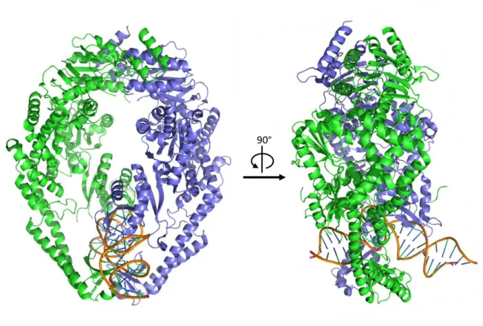
Figure 1.2: Crystal Structure of Taq MutS.
6 Error Recognition by Thermus aquaticus MutS
MutS Structural Information
Errors in the genome are vastly outnumbered by properly base-paired (homoduplex) DNA, making error recognition an enormous challenge. This monumental task is undertaken by MutS and the MutS homologs. In Taq, MutS forms an obligate homodimer (hereafter referred to as MutS) that contains a DNA binding domain and two adenosine nucleotide binding sites. Upon binding DNA, the homodimer becomes asymmetric, and this asymmetry is conferred to the nucleotide binding sites. As is apparent in the crystal structure (Figure 1.2), MutS induces a significant bend in the DNA of approximately 60 degrees at the mismatch. This kink in the DNA is thought to be important for mismatch recognition, as the DNA near the error is expected to be more inherently flexible. By better tolerating protein-induced DNA bending, the position of the error becomes a localized energy minimum. Upon binding to the site of the error, the erroneous base is rotated 3Å out into the minor groove of the double helix and stacks with a conserved phenylalanine residue in the DNA binding domain of MutS (Obmolova et al., 2000). Taq MutS retains some affinity for homoduplex DNA (KD = 20-35 µM), though, as a result of the specific
interactions formed upon error recognition, MutS has a greater affinity for DNA containing a mismatch (KD = 5-40 nM) (Yang, Sass, Du, Hsieh, & Erie, 2005).
The Role of DNA Bending in Error Recognition by MutS
7
the “unbent” population was only found at the position of the GT mismatch or T-bulge, and the
protein:DNA complexes observed on homoduplex DNA were all found to be bent. These results led to the development of a model wherein a mismatch-dependent “bent” to “unbent” transition was proposed to be vital for signaling downstream MMR events (Wang et al., 2003).
A single-molecule fluorescence study in our lab further explored DNA bending conformations adopted by Taq MutS:DNA complexes. Six different DNA-bending conformations were identified using DNA containing a GT mismatch, two of which correspond to the “bent” and “unbent” populations seen in the AFM studies. Importantly, this study revealed that MutS-induced DNA bending is highly dynamic, and certain transitions between states were preferentially observed, most notably the “bent” to “unbent” transition (Sass, Lanyi, Weninger, & Erie, 2010). Subsequent single-molecule fluorescence studies on DNA substrates containing either a T-bulge or a CC mismatch revealed that preservation of this “bent” to “unbent” transition correlated with repair efficiencies (Derocco, Sass, Qiu, Weninger, & Erie, 2014).
These data, taken together, suggest that error recognition by Taq MutS in the absence of ATP can occur through the following mechanism: MutS first binds to and bends homoduplex DNA and then slides along the DNA until it encounters the error. Once at the error, MutS bends the DNA into the initial recognition complex observed in the crystal structure. The MutS:DNA complex can then undergo a series of dynamic conformational changes that leads to the formation of the ultimate recognition complex in which the DNA is unbent (Wang et al., 2003).
ATP-induced Conformational Changes in Taq MutS
8
2015). While the existence of this state is well established, its purpose remains unclear. The sliding clamp is thought to be involved one or more downstream events of MMR, such as recruitment of MutL or an exonuclease. The purpose of the sliding clamp may also be to clear the error site for recognition by a second MutS and/or searching for the strand discrimination signal.
Formation of Taq MutS:MutL:DNA Ternary Complexes
Following error recognition, MMR initiation continues in all species with the ATP-dependent recruitment of MutL to the mismatched site by MutS. The Taq MutL homodimer (in humans, the
heterodimer MutLα) is then responsible for nicking the error-containing daughter strand on either side of the error. To accomplish this task, the N-terminal domain of each MutL monomer has a DNA binding domain, while the C-terminal domain has endonuclease activity. These two domains are connected by a flexible linker that is thought to be intrinsically disordered. While X-ray crystallography has provided structural information for the N- and C-terminal domains of E. coli MutL (Ban, Junop, & Yang, 1999), a structure of full length MutL for any species has remain elusive, likely as a result of the disordered linker region.
9
10
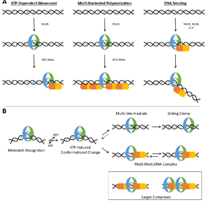
Figure 1.3: Models of MutS:MutL:DNA Ternary Complexes.
11 Single-molecule Fluorescence
Few tools are able to track the molecular events of complex biological processes; however, single-molecule fluorescence techniques are well suited for such studies. Unlike their bulk fluorescence counterparts, observations made using single-molecule techniques are not limited to the ensemble
average. Rather, single-molecule methods are well suited for studying systems where the average does not represent any species. In addition, single-molecule methods are able to reveal relatively rare or transient events whose contributions to the ensemble would otherwise be hidden beneath the signals from more dominant populations in the ensemble. These rare or transient events are often vital to understanding the detailed molecular mechanisms behind complex, heterogeneous, and asynchronous molecular biology processes, such as DNA mismatch repair (Erie & Weninger, 2014; Gell, Brockwell, & Smith, 2006; Lakowicz, 2006).
Single-molecule Fluorescence Resonance Energy Transfer (smFRET)
12 𝐸 = 1
(1+𝑟6 𝑅06)
Eq. 1.1
where r is the interfluorophore distance and R0 is known as the Forster radius. Due to the 1/r6 relationship
shown in Eq. 1, FRET efficiency is exquisitely sensitive to changes in interfluorophore distance (Gell et al., 2006; Lakowicz, 2006).
The Förster radius R0 is defined for a given pair of fluorophores as the interfluorophore distance
at which the FRET efficiency is 50%. Importantly, R0 represents the orientational-, spectral-, and
quantum yield-dependence of FRET; thus, every FRET pair of fluorophores will have a unique Förster radius depending on these properties. Furthermore, since the fluorophore orientations, spectral properties, and quantum yields all depend on the local environment of the fluorophores, the Förster radius of a given FRET pair can vary depending on the labeling strategies and experimental conditions. Practically, however, these conditional variations are difficult to predict (Lakowicz, 2006).
When exciting only the donor fluorophore of a FRET pair, any emission from the acceptor dye will be indicative of FRET. Thus, the energy transfer efficiency can be described as fraction of the total detected intensity (i.e. the intensity of both the donor and acceptor) due to emission from the acceptor. Mathematically, this relationship is described as:
𝐸 = 𝐼𝐴
𝐼𝐷+𝐼𝐴 Eq. 1.2
where IA and ID are the intensities of the acceptor and donor fluorophore emissions, respectively.
13
donor and acceptor intensity when there are changes in transfer efficiency. Thus, a more exact description of smFRET is:
𝐸 = 𝐼𝐴−𝛼𝐼𝐷
𝛾𝐼𝐷+(𝐼𝐴−𝛼𝐼𝐷) Eq. 1.3
where IA and ID are the raw, uncorrected intensities of the acceptor and donor fluorophore emissions,
respectively. The α term accounts for leakage of a fraction of the donor signal into the acceptor signal. The factor γ corrects for the photophysical differences between the dyes and can be defined as:
𝛾 = 𝜑𝐴𝜂𝐴
𝜑𝐷𝜂𝐷 Eq. 1.4
where φA and φD represent the quantum yields of the acceptor and donor fluorophores, respectively, and
ηA and ηD represent the detection efficiencies of the acceptor and donor fluorophores, respectively (Gell et
al., 2006; Lakowicz, 2006; McCann, Choi, Zheng, Weninger, & Bowen, 2010).
Total Internal Reflection Fluorescence Microscopy
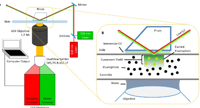
Emissions from single fluorophores are often sufficiently bright for modern detection technology; however, distinguishing the fluorophore emission from the background is much more challenging. Total internal reflection fluorescence (TIRF) microscopes are able to selectively excite only those fluorophores within ~200 nm of the surface of a slide by exploiting differences in the refractive index properties of the optical components and slides. Two optical setups for TIRF microscopes exist: through-prism and through-objective (Gell et al., 2006). This work was completed using a through-prism setup (Figure 1.4A).
When an excitation beam of light hits the interface of two materials with differing refractive indeces (n1 and n2), it can either be reflected or transmitted (possibly with some refraction). Total internal
14 𝜃𝑐 = sin−1(
𝑛2
𝑛1) Eq. 1.5
At the point of reflection (Figure 1.4B), an electric field referred to as the evanescent field is created, which propagates through the interface. The intensity of this evanescent field decays exponentially as the distance from the interface increases according to the following relationship:
𝐼(𝑧) = 𝐼(0)𝑒(−𝑑𝑧) Eq. 1.6
where I(z) is the intensity of the evanescent field at a distance z from the interface. I(0) is the intensity of evanescent field at the interface (i.e. where z = 0), and d is the penetration depth. The penetration depth of an evanescent field depends on several factors, including the refractive indices of the two materials (n1
and n2) and the wavelength and incidence angle of the excitation light (Gell et al., 2006; Lakowicz, 2006).
Figure 1.4: TIRF Microscopy.
15
In practice, a quartz (n1 = 1.55) slide and prism are used, and biological samples are typically
studied in aqueous environments (n2 = 1.33). 532 and 638 nm are common wavelengths of lasers used for
excitation in smFRET experiments. Given these parameters and a 60° angle of incidence, the predicted penetration depths for the two excitation beams are 233 and 278 nm for 532 and 638 nm laser beams, respectively. Remembering that the evanescent wave decays exponentially as distance from the
quartz:water interface increases, only those fluorophores very close to the slide (~200 nm) are sufficiently excited. By limiting off-target excitation in this way, background fluorescence is minimized.
Thesis Statement
This thesis aims to characterize the nucleotide dependence of Thermus aquaticus MutS-induced DNA bending throughout sliding clamp formation during mismatch repair initiation. The current model for MutS conformational changes that occur upon error recognition will be expanded to include DNA bending information. Largely, this aim will be achieved through the use of single-molecule fluorescence resonance energy transfer experiments designed to be sensitive to changes in DNA bending. Finally, a data analysis pipeline has been developed to streamline the analysis as well as optimize detection of small, yet significant changes in FRET.
16
CHAPTER 2: A GUIDE TO MONITORING PROTEIN-INDUCED DNA BENDING BY smFRET
Introduction
Protein-induced DNA bending is used as a signaling mechanism in many molecular biological processes, such as DNA mismatch repair (Iyer et al., 2006; Kunkel & Erie, 2005). Thus, measuring the extent of DNA bending, identifying DNA bending states, and characterizing the dynamics of exchange between these states can provide mechanistic insight into these processes. Several structural methods for observing protein-induced DNA bending exist, including atomic force microscopy and x-ray crystallography, but these methods are limited to static images of the protein:DNA complexes. Single-molecule fluorescence resonance energy transfer (smFRET), however, is able to sensitively detect changes in DNA bending in real time. This technique provides kinetic and conformational information that can elucidate the molecular details of these processes (Derocco et al., 2014; Erie & Weninger, 2014; Sass et al., 2010).
17 Designing Fluorescently Labelled DNA Oligonucleotides
When monitoring protein-induced DNA bending, the oligonucleotide labeling strategy must be thoughtfully designed such that the fluorescent properties of the fluorophores are sensitive to changes in the DNA conformation. Also, fluorescently labelled oligonucleotides are quite expensive (e.g. several hundred dollars per 100 nanomoles). Therefore, it is important to take care when deciding where and how to label the DNA. The specific fluorophores used, the position of the fluorophores on the DNA, and the fluorophore attachment chemistries have significant impacts on the sensitivity of the DNA substrates’ fluorescent properties. Each of these parameters is discussed below.
Selecting the Fluorophores
There are several fluorescent tags that are commercially available for labeling oligonucleotides (e.g. TAMRA, the Cy dyes, Alexa dyes, and many others). When choosing which specific fluorophores to use, it is important to select dyes that have high quantum yields so they can be more easily detected. Also, the dyes’ excitation and emission spectra should be compatible with your optical setup such that independent excitation and emission detection for each dye is possible. For FRET between the dyes to be possible, the emission spectrum of the donor fluorophore must overlap with the excitation spectrum of the acceptor fluorophore. Donor-acceptor dye pairs commonly used to label DNA in smFRET experiments include: Alexa 555-Alexa 647, TAMRA-Cy5, and Cy3-Cy5 (Derocco et al., 2014; Qiu et al., 2012, 2015; Sass et al., 2010).
18
them poor choices for monitoring DNA bending. Finally, some dyes are prone to interactions with the DNA (e.g. stacking with the nitrogenous bases), which may change their fluorescence properties in ways that do not depend on DNA bending or any other property. Due to these factors, it is often best to use a pair fluorophores which have proven successful in other experimental contexts.
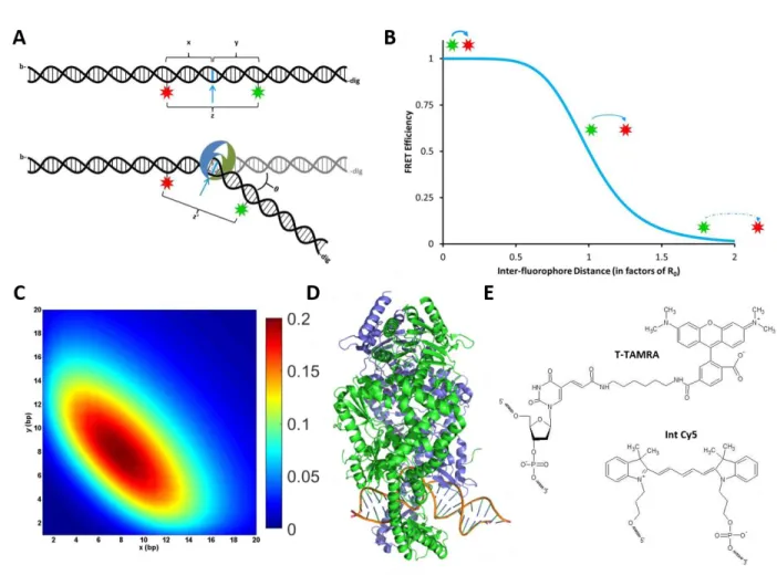
Figure 2.1: Considerations for Designing Fluorescent Oligonucleotides to Study DNA Bending A) A schematic of a doubly-labeled oligonucleotide sensitive to changes in DNA bending. Donor (green) and acceptor (red) fluorophores flank either side of a site of protein-induced DNA bending (blue arrow). B) FRET curve showing the relationship between inter-fluorophore distance and FRET efficiency. C) Heat map showing the predicted change in FRET (according to the color scale) for oligonucleotides labeled in different positions (x and y from panel A). These simulations used the following parameters: θ = 60°, R0 =
19 Optimizing the Fluorophore Positions
Consider an oligonucleotide that is bent upon protein binding (Figure 2.1A) (Derocco et al., 2014; Sass et al., 2010). Such protein-induced bend in the DNA brings the two flanking arms of the DNA (x and y) nearer to each other. Thus, if a DNA substrate is labelled with a donor and acceptor fluorophore on either side of a site of protein-induced DNA bending (Figure 2.1A), the induced DNA bend angle (θ) will decrease the interfluorophore distance (from z to zʹ) thereby increasing the FRET efficiency between the two dyes. The sensitivity and reliability of this increase in FRET can be optimized by considering several parameters, including the predicted bend angle, the placement of the dyes relative to the site of DNA bending, and the protein footprint.
Changes in interfluorophore distance cause changes in FRET efficiency (E) following the equation:
𝐸 = 1 1+(𝑟
𝑅0)
6 Eq. 2.1
where r is the interfluorophore distance and R0 is the Förster radius of the donor:acceptor fluorophore pair
(Figure 2.1B) (Gell et al., 2006; Lakowicz, 2006).
More significant bend angles (θ) will produce larger changes in interfluorophore distance, and thus, larger changes in FRET efficiency. Placing the fluorophores far from the site of bending (large values of x and y), will increase the change in interfluorophore distance before and after bending (z-zʹ); however, because FRET efficiency is related to (1/r)6, large changes in interfluorophore distance will not always
result in large changes in FRET efficiency. If z >> R0 or if z << R0, the FRET efficiency will not change
significantly upon bending. Instead, placing the dyes such that the FRET efficiency is near 0.2-0.4 (i.e. z > R0) in the absence of DNA bending is best. From this position, even small changes in DNA bending will
decrease the interfluorophore distance, causing large changes in FRET efficiency.
20
every combination of labeling positions (x and y), base-by-base along the DNA (Figure 2.1C). In the resulting heat map, warmer colors indicate regions of the greatest change in FRET upon bending. A clear maximum is observed when both fluorophores are placed 8 base pairs from either side of the site of DNA bending.
Note that this simulation is limited by several factors. The calculations require prior knowledge of the expected bend angle as well as the Förster radius for the FRET pair used. The bend angle may be known if structural information (i.e. a crystal structure) of your protein:DNA complexes of interest is available. Förster radii are available for several FRET pairs, but these values are determined using fluorophores free in solution. Attachment to DNA can change the properties of the dyes, so it is impossible to know how the exact Förster radius of a given FRET pair in these contexts. Also, this simulation does not account for DNA twisting that may occur during DNA bending, nor does it consider slight differences in interfluorophore distance caused by placing both fluorophores the same DNA strand or on opposite strands of the helix. These simplifications are used, in part, because protein-induced twisting and its effects on changes in interfluorophore separation are difficult to predict.
21 Choosing the Fluorophore Attachment Chemistry
Several chemical strategies exist to link fluorophores to the DNA (Figure 2.1E). Labeling the 5ʹ- or 3ʹ-ends of the DNA is one option; however, being limited to only the ends of the DNA may be problematic. While internally labeling DNA oligonucleotides provides much more flexibility in choosing labeling positions, fewer commercially available options for fluorophores exist. There are two major types of internal labels: 1) fluorophores are covalently attached to thymine bases via a flexible carbon linker extending from the major groove in the DNA, and 2) certain dyes (e.g. the Cy dyes) can be incorporated directly into the DNA backbone. Note that these backbone fluorophores are rigidly locked into a specific orientation relative to the DNA backbone as they are covalently attached at both ends. Conversely, fluorophores on a flexible linker have more conformational freedom. As the Förster radius of a given FRET pair of fluorophores depends, in part, on the relative orientation of the transition dipoles of the two fluorophores (Lakowicz, 2006), limiting both fluorophore moieties’ conformational freedom may lead to unpredictable changes in FRET upon DNA bending due to changes in their relative orientations. For more predictable changes in FRET, at least one freely rotating dye (i.e. those attached to flexible linkers) is recommended.
Other Considerations
22
In several studies, blocking the ends of the DNA may be experimentally useful, such as when studying proteins that are topologically linked around the DNA. To prevent dissociation of such proteins from the end of the DNA oligonucleotides, the ends must be blocked. One end of the DNA is blocked by the slide surface. By attaching a digoxigenin moiety to the 5ʹ-end of the unbiotinylated strand, end-blocking can be achieved using an anti-digoxigenin antibody (Qiu et al., 2012, 2015).
Optical Setup and Data Collection
23 Figure 2.2: Optical Setup and Data Analysis Pipeline.
A) An example total internal reflection fluorescence microscopy set up suitable for the described DNA bending measurements. B) A schematic of the data analysis pipeline.
Data Analysis
24
Extracting the Fluorescence Time Traces of Individual DNA Molecules
Data acquisition by the aforementioned setup produces a movie made up of approximately 1000 frames. Each frame contains the fluorescence emission intensity gathered over a period of time for 512 X 512 pixels using a DualView splitter, the emissions from the donor and acceptor dyes are projected to the right and left halves, respectively, of each frame (Figure 2.2B, Top). So long as the slides are not overloaded with DNA substrate, emissions from each individual DNA molecule appears as two distinct foci (a focus from the acceptor emission on the left half and a focus from the donor emission on the right).
By initially exciting only the acceptor dye, local maxima on the left half of the image can be identified. The pixel coordinates of these maxima represent the positions of the DNA molecules within the image. These same pixel coordinates mapped to the other half of the frame should locate the emissions from the donor dye; however, the two halves of each frame must first be aligned to one another to account for misalignments in their optical paths. To determine the relative offset between the two halves of the image, beads with a broad emission spectra are imaged. These images allow an experimentally determined offset to be determined, which is then applied to the experimental movies.
25 Correcting the Donor and Acceptor Signals
Emissions from the donor and acceptor must be corrected to account for differences in the photophysical properties of the dyes. First, it is important to note that the donor and acceptor fluorescence emission spectra may not be completely distinct. That is to say that despite using optical filters and dichroic mirrors to separate emissions from the two dyes, the donor dye may still emit at wavelengths assigned to the acceptor. Even though these emissions are likely not large, they may still introduce significant error. This “leakage” into the acceptor detection window is proportional to the donor intensity. Thus, a proportionality constant can be empirically determined and used to subtract the “leaked” donor signal from the acceptor intensity at each time point using the following equation:
𝐼𝐴,𝑐𝑜𝑟= 𝐼𝐴,𝑟𝑎𝑤− 𝛼𝐼𝐷,𝑟𝑎𝑤 Eq. 2.2
where α represents the leakage proportionality constant, IA,raw and IA,cor are the raw and corrected acceptor
intensities, respectively, and ID,raw is the raw donor intensity at each time point (Gell et al., 2006; Lakowicz,
2006).
Additionally, the donor and acceptor dyes may have different quantum yields and/or different detection efficiencies. These differences can be corrected using a method described by McCann et al. using an empirically determined gamma factor by the following equation:
𝐼𝐷,𝑐𝑜𝑟 = 𝛾𝐼𝐷,𝑟𝑎𝑤 Eq. 2.3
where γ represents the empirically determined correction factor. IA,raw and IA,cor are the raw and corrected
26
Smoothing the Donor and Acceptor Time Traces Using the Chung-Kennedy Filter
Due to the sensitivity of single-molecule detection, the resulting fluorescence intensity time traces have relatively high noise. This noise is problematic when monitoring small changes in FRET. Consequently, if the change in DNA bending is small, it can be difficult to detect such changes in noisy data. Several methods exist to smooth noisy data, such as box-car averaging, but most of these smoothing methods do not preserve sharp edges, making the transition even more difficult to detect.
To overcome this limitation, Chung and Kennedy developed a non-linear smoothing algorithm designed specifically to smooth data while preserving edges (Chung & Kennedy, 1991; Haran, 2004). This algorithm smoothes data containing transitions (Figure 2.3A) by first determining the averages for windows of data of various size on either side of a given data point (dubbed the “forward” and “backward” average windows, Figure 2.3B). To preserve edges, “forward” and “backward” averages that contain transitions are given less weight in the overall average. The statistical weights assigned to the “forward” and “backward” averages are determined as follows: The standard deviations for windows of data on either side of the data point being smoothed (referred to as the “forward” and “backward” predictor windows, Figure 2.3C) are determined. The inverse of these standard deviations raised to a user-defined exponential term p are then used to calculate the statistical weights.
27 Figure 2.3: Chung-Kennedy Smoothing Algorithm.
A) An example of data containing a transition between t + 2 and t + 3. B) A schematic depicting three sizes of “forward” (green) and “backward” (red) average windows. C) A schematic depicting 4-point “forward” (green) and “backward” predictor windows.
28
average window size(s), predictor window size(s), and exponent term(s) can be defined by the user, and the optimal values in a given application can be empirically determined. Over filtering (i.e. introduction of false transitions) can be minimized by optimizing these input parameters.
When properly applied to the donor and acceptor time traces, the signal-to-noise ratio is significantly improved (Figure 2.2B, Third Row), and transitions in the data are clearer. Notably, in single-molecule FRET experiments, transitions in the donor and acceptor traces are expected to be anti-correlated (i.e. if the donor intensity increases, the acceptor intensity should simultaneously decrease, and vice versa). Because transitions in the donor and acceptor traces are expected to be simultaneous, the Chung-Kennedy smoothing algorithm can be improved by using the sum of the predictor window standard deviations for the both the donor and acceptor to determine the statistical weights. As a result, simultaneous donor and acceptor intensity transitions will be more strongly preserved compared to uncorrelated donor and acceptor changes in intensity (Haran, 2004).
Screening Time Traces for Data Quality
To expedite analysis of large amounts of single-molecule data, time traces of insufficient quality should be discarded from further analysis. There are several reasons a time trace or portions of a time trace may not be worth analyzing. For example, the detected fluorescence emission intensities may be too low to reliably detect changes in intensity, or they may be too high to represent emission from only one molecule. More commonly, either the donor or acceptor fluorophore (or both) may permanently or temporarily loose its fluorescence properties (i.e. bleach or blink) during data acquisition.
29
determine a 95% confidence interval for each data point. If this interval includes zero, the data point can be considered as part of a bleaching or blinking event and discarded from analysis.
Time traces made up entirely of data points that cannot be analyzed can be discarded out right. Those containing both analyzable and unanalyzable regions, however, may contain useful information (e.g. prior to photobleaching). While this screening process greatly increases the efficiency of data processing, false-positives and/or false-negatives may occur. For example, individual data points in analyzable regions may be falsely identified as unusable by this method. For this reason, the quality of each data point can be iteratively compared to its neighboring data points and, in the event of discrepancies, changed to conform to its neighbors.
Calculating FRET and Identifying Transitions in the FRET Time Traces
Regions of the remaining donor and acceptor time traces that are of sufficient quality to analyze can then be used to calculate single-molecule FRET efficiency using the following equation:
𝐸 = 𝐼𝐴
𝐼𝐴+𝐼𝐷 Eq. 2.4
where IA and ID represent the corrected and smoothed fluorescence emission intensities of the acceptor and
30
Several methods exist to detect transitions in data, though each has its own limitations. False-positives (i.e. finding transitions that do not exist) and false-negatives (i.e. missing transitions that should be detected) can both hinder interpretation of the data. Applying the same transition detection method at different levels of stringency can minimize these mistakes, as transitions that withstand more stringent thresholds are more likely to be “real”. Comparing the results of multiple methods, can also help to overcome the limitations of using just one technique, as different detection methods will be better suited for detecting different types of changes (e.g. short- vs. long-lived states) and will have different limitation. Edges detected by multiple methods at multiple stringency levels can then be assigned a higher confidence score. Presented here are two transition detection methods that can be independently applied at multiple thresholds to smFRET data.
Method 1: The Gaussian Kernel Method (Sass et al., 2010)
Mathematically, transitions in continuous functions can be identified by finding inflection points (i.e. maxima and minima in the first derivative of the time trace). Unfortunately, the FRET time traces are made up of discrete data points that have many apparent inflection points due to the significant noise in the signal. These issues can be circumvented by first convolving the FRET time traces with a Gaussian kernel of various widths and subsequently detecting inflection points in the convolved data. To ensure only “real” transitions are kept, a threshold can be incorporated. By changing the rigor of the threshold, the remaining “real” transitions can also be scored for confidence.
Method 2: The Chung-Kennedy Method
31
Figure 2.4: A Novel Transition Detection Method Based on the Chung-Kennedy Filter.
32
Consider a data point at time t with a transition occurring between time t + 2 and t + 3 (Figure 2.4). Using a predictor window of 4 data points, the standard deviation of both the forward and backward predictor windows can be calculated at each value of t. (Figure 2.4 depicts these calculations for t - 2 to t + 7.) In this example, the standard deviation of the forward predictor window at time t is at a local maximum. This also occurs in backward predictor window at time t + 5 because these windows contain the same range of data points. Thus, transitions can be detected by finding the midpoint between local maxima in the standard deviations of the forward and backward predictor windows. To ensure only “real” transitions are kept, only the highest percentile local maxima (e.g. 95th-99th percentile) are considered. By changing this
percentile, the transitions can then be scored for confidence.
Notably, this method’s ability to detect transitions is depends on the noise in the FRET time traces, as those traces with low signal-to-noise will have inherently high standard deviations, confounding the results. The most common source of false-positives is bleaching and blinking events where either the donor or acceptor fluorescence intensity is approximately zero. Very low donor or acceptor intensity can cause the FRET time trace to be very noisy, oscillating between 1 and 0. To circumvent this issue, regions of data previously identified as bleaches and blinks can be assigned a constant FRET (e.g. 0 or -1), which eliminates their standard deviations and allows this transition detection method to function properly.
Alignment and Confirmation of Transitions in the FRET Time Traces
33
Both of the methods described here require user input to choose the appropriate thresholds. In the event that transitions are being missed (false-negatives), the thresholds ought to be made less stringent. More often, though, too many “unreal” transitions are identified (false-positives). To test the significance of each transition, the FRET efficiency between each transition can be averaged, and the averages of adjacent FRET states can be subjected to a t-test. If two states are deemed not statistically significantly different from one another (p level 0.05), then the transition between the two states can be identified as a false-positive and discarded.
User Interaction and FRET-TACKLE
The resulting set of transitions (Figure 2.2B, Bottom Row) represents a best approximation of the simultaneous donor and acceptor changes in intensity. In the analysis described so far, the user is only required for the initial input parameters, such as smoothing windows and transition detection thresholds; the rest of the analysis can be completed by a computer in batch. Upon completion of the batch analysis, the computationally discovered transitions can be verified by the user, and any remaining false-positives in each molecule’s FRET time trace can be discarded by hand. This process, though tedious, can be crucial to recognizing patterns or detecting systematic errors in the computational approach.
34 Conclusion
35
CHAPTER 3: CHANGES IN DNA BENDING CORRELATE WITH MUTS CONFORMATIONAL CHANGES DURING SLIDING CLAMP FORMATION
Introduction
Errors introduced during DNA replication must be corrected to maintain genomic stability. DNA mismatch repair is a biochemical pathway that increases the fidelity of DNA replication 100-fold by correcting misincorporated bases or insertion/deletion loop errors. The proteins involved in mismatch repair proteins are also involved in a range of other biochemical processes, including DNA damage response and double strand break repair. Unsurprisingly, mutations in the mismatch repair proteins are associated with several types of cancer, including certain hereditary nonpolyposis colorectal cancers (Iyer et al., 2006; Kunkel & Erie, 2005).
36
Recent studies using single-molecule fluorescence resonance energy transfer (smFRET) successfully characterized the conformational and kinetic properties of Taq MutS during sliding clamp formation (Jeong et al., 2011; Qiu et al., 2012, 2015). In these studies, MutS was tagged with a donor fluorophore and the DNA containing an error tagged was tagged with an acceptor fluorophore such that when MutS bound to the error, FRET between the dyes could occur. In the presence of saturating ATP, Taq MutS bound to the error in a state with high FRET. Qiu et al. observed that a subset of these mismatch-binding events (~20%) underwent a preferred pathway of changes in FRET (high FRET intermediate FRET zero FRET). These changes were attributed to sliding clamp formation, as the final zero FRET could only occur if MutS had moved away from the acceptor dye (i.e. far from the mismatch) while still bound to the DNA. In addition, kinetic analysis of the total time MutS spent bound to T-bulge substrates yielded a characteristic lifetime of 11.7 sec (Qiu et al., 2012, 2015). In additional experiments, the DNA binding domains of each monomer of MutS was labeled with one dye from a FRET pair. Using this method, conformational changes within the MutS dimer were identified during sliding clamp formation. Importantly, the lifetimes associated with the states identified in the intramolecular FRET experiments correlated with those observed in the protein-to-DNA FRET experiments (Qiu et al., 2012).
37
DNA bending throughout the process of sliding clamp formation without evidence for these changes (Qiu et al., 2012, 2015).
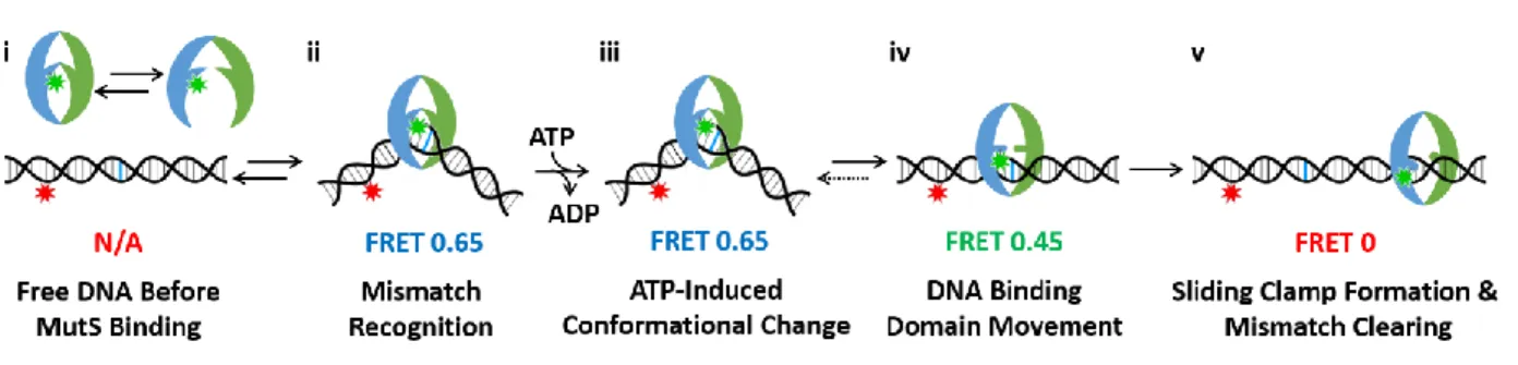
Figure 3.1: The existing model of sliding clamp formation by Taq MutS.
(i) Prior to binding DNA, MutS exists in a conformational equilibrium. (ii) MutS binds and bends the DNA at the error. MutS adopts a conformation where the two DNA binding domains are near each other. (iii) MutS exchanges ADP for ATP, and the conformation changes little. (iv) MutS undergoes a conformational change that slightly opens the DNA binding domains. (v) The DNA binding domains fully open as MutS becomes a sliding clamp and moves away from the mismatch. Adapted from (Qiu et al., 2015).
DNA bending by Taq MutS has been well characterized by X-ray crystallography and atomic force microscopy (Alani et al., 2003; Obmolova et al., 2000; Wang et al., 2003). This MutS-induced DNA bending is not static, and several single molecule studies have dissected the DNA bending dynamics of MutS:DNA complexes in the absence of adenosine nucleotides (Derocco et al., 2014; Sass et al., 2010). In these studies, a key “bent-to-unbent” transition has been identified, and preservation of this transition correlates with efficient repair (Derocco et al., 2014; Wang et al., 2003). However, little is known about the nucleotide dependence of these DNA bending conformations, nor is the contribution of DNA bending throughout process of forming the sliding clamp well understood. To fully understand the actions of MutS in mismatch repair initiation, we must elucidate the molecular changes occurring in both MutS and the DNA.
38
correlated to the previous smFRET studies via their characteristic kinetics. Notably, a pathway of DNA bending states was identified, and the kinetics of this pathway correlate well with the sliding clamp formation kinetics from the previous studies. Moreover, a conformational change previously identified only by kinetic analysis was characterized by changes in the DNA bending conformation. We then refine the model for sliding clamp formation to account for conformational changes in both MutS and the DNA.
Results
To study the nucleotide dependence of MutS-induced DNA bending during sliding clamp formation using smFRET, we designed a 68 bp oligonucleotide that is doubly-labeled with a FRET pair of dyes, TAMRA (donor) and Cy5 (acceptor). These dyes are separated by 19 bp flanking a single thymine insertion error (referred to herein as T-bulge) near the midpoint of the oligonucleotide (Figure 3.2A). This oligonucleotide is also biotinylated on one end so that it could be immobilized via an interaction with streptavidin-biotinylated BSA on the surface of a quartz slide. The cysteine mutant C42A/M88C Thermus aquaticus MutS with wild type ATPase and DNA binding activities is used in this study to allow for direct comparison to existing smFRET data (Qiu et al., 2012, 2015).
MutS:ADP bends DNA to a single bent conformation.
39
was observed to transition between only two distinct FRET states, a low FRET state (Figure 3.2B, red arrows) and a high FRET state (Figure 3.2B, cyan arrows). A histogram of the average FRET efficiency of the low FRET states (Figure 3.2C, red bars) shows a peak centered around 0.25, similar to the free DNA distribution. A histogram of the average FRET efficiency of the high FRET states in each trace (Figure 3.2D) is shifted to higher FRET with a peak centered around 0.35. This result is consistent with MutS-induced DNA bending upon binding to DNA containing a T-bulge, as was observed previously in the absence of ADP (Derocco et al., 2014; Sass et al., 2010; Wang et al., 2003). The FRET transitions detected in these transitions are depicted in a transition density plot (TDP), where warmer colors represent more frequent transitions (Figure 3.2E). Two dominant types of transitions are observed: (1) a low FRET state transitioning to a high FRET state, and (2) a high FRET state transitioning to a low FRET state.
Using the observed change in FRET efficiency and the law of cosines, the DNA bend angle can be calculated; however this calculation is complicated by variations in the Förster radius caused by linking the fluorophores to the DNA and fluorophore-DNA interactions. If these complications are ignored, the observed change in the average FRET efficiency from ~0.25 to ~0.35 corresponds to a DNA bend angle of ~45°, which agrees well with the DNA bend angle observed in the crystal structure and in the AFM studies (Alani et al., 2003; Obmolova et al., 2000; Wang et al., 2003).
40
Figure 3.2: In the presence of ADP, Taq MutS bends T-Bulge DNA to a single bent state.
41
In the presence of ATP, most MutS:DNA complexes adopt a single bent conformation.
To ascertain how the conformation of the DNA changes upon introduction of ATP, we monitored the smFRET efficiency of our doubly labeled oligonucleotide (Figure 3.2A) in the presence of Taq MutS and saturating concentrations of ATP. Again, anti-correlated changes in the donor and acceptor fluorescence intensity time traces are observed when MutS and ATP are added. Dynamic changes in the FRET efficiency were observed (Figure 3.3A). In the majority of these events (70%), only two FRET states were observed: a low FRET state (Figure 3.3A, red arrows) and a high FRET (Figure 3.3A, cyan arrows), similar to the ADP FRET time traces. Histograms of the average FRET efficiency of each state show that the low FRET state (Figure 3.3B, red bars) exhibits a peak centered around 0.25. This peak is slightly broader than that observed in the presence of ADP but is still quite similar to the free DNA FRET distribution (Figure 3.3B, black dotted cityscape). The high FRET distribution observed in the presence of ATP (Figure 3.3C) was shifted to higher FRET with a peak centered around 0.4. This distribution is also broader than the high FRET distribution observed in the presence of ADP, perhaps due to MutS being inherently more dynamic in the presence of ATP.
42
For this subset of transitions, the distribution of dwell time in the high FRET state (Figure 3.3E, cyan bars) fit well to a single exponential decay (Figure 3.3E, black line), yielding a characteristic lifetime of 4.2 ± 0.6 sec, within error of the lifetime observed in the presence of ADP and very close to that observed previously (2.7 sec) (Qiu et al., 2012, 2015).
Figure 3.3: In the majority of Taq MutS:DNA complexes formed in the presence of ATP, the DNA adopts a single bent state.
43
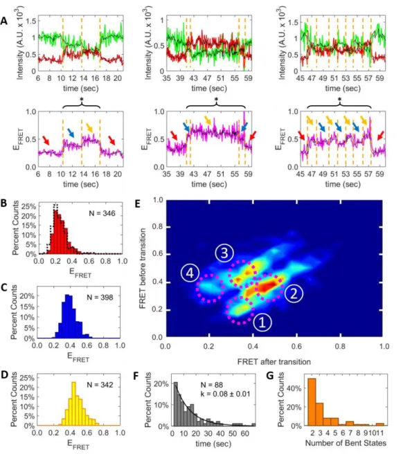
ATP induces a subset of MutS:DNA complexes to adopt multiple conformations.
In the remaining subset (30%) of the DNA bending events observed in the presence of Taq MutS and ATP, more than two FRET states are observed: a low FRET state, an intermediate FRET state, and a high FRET state (Figure 3.4A, red, blue, and yellow arrows, respectively). The distribution of FRET values for the low FRET state (Figure 3.4B, red bars) is again similar to the free DNA FRET (Figure 3.4B, black dotted cityscape), as both exhibit a peak centered around 0.25. The average FRET efficiency peaks for the intermediate and high FRET states (Figures 3.4C and 3.4D, respectively) are centered around 0.35 and 0.45, respectively. Such shifts in the FRET values predict DNA bend angles of ~45° and ~60°, respectively. These results are consistent with the previously observed range of Taq MutS:DNA complex conformations with distinct extents of DNA bending in the absence of nucleotides using T-bulge DNA ( Alani et al., 2003; Obmolova et al., 2000; Derocco et al., 2014; Wang et al., 2003).
Examination of the TDP (Figure 3.4E) reveals four major transitions: (1) a low FRET state transitioning to an intermediate FRET state, (2) an intermediate FRET state transitioning to a high FRET state, (3) a high FRET state transitioning back to an intermediate FRET state, and (4) an intermediate FRET state returning to a low FRET state. Notably, the systematic error responsible for broadening the peaks in the TDP of the events with a single bent (Figure 3.3D) is again apparent in the TDP for the events transitioning through multiple bent states.
44
Figure 3.4: In a subset of Taq MutS:DNA complexes formed in the presence of ATP, switching between multiple bent states is observed.
45
DNA bending by MutS:ATP follows a preferred pathway of transitions.
In the events with multiple bent states, the number of intermediate and high FRET states entered before returning to the low FRET state (Figure 3.4F) shows a preference for fewer transitions. Approximately 75% of the events with multiple bent states adopt only two or three bent FRET states before returning to the low FRET state (Figure 3.5A). Rarely, the FRET oscillates between the high and intermediate FRET states 4 or more times before returning to the low FRET state (Figure 3.4A, right column).
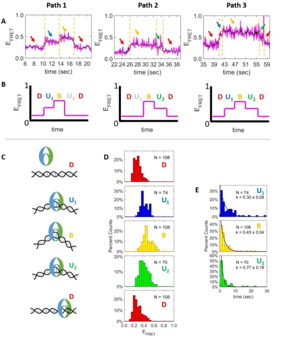
The events adopting only two or three bent FRET exhibit a three preferred transition paths: Path 1) low FRET intermediate FRET high FRET low FRET (Figure 3.5A, left), Path 2) low FRET high FRET intermediate FRET low FRET (Figure 3.5A, middle), and Path 3) low FRET intermediate FRET high FRET intermediate FRET low FRET (Figure 3.5A, right). As depicted in the simplified schematics (Figure 3.5B), Paths 1 and 2 may represent subsets of Path 3 where one conformation was not observed. Using this model, each state is assigned an extent of MutS-induced DNA bending based on the FRET value as follows: Low FRET states (Figure 3.5A, red arrows) are assumed to be linear DNA (Figure 3.5C, D). This assumption is supported by the FRET distribution of these states (Figure 3.5D, red bars D), which is centered around 0.25 similar to free DNA. The intermediate FRET states (Figure 3.5A, blue arrows) are attributed to slightly bent DNA (Figure 3.5C, U1 and U2) because their
FRET distributions (Figure 3.5D, blue bars and green bars for U1 and U2 respectively) have shifted to higher
FRETs and are centered around 0.35. Interestingly, the FRET associated with U2 appears to be significantly
broader than that of U1. Finally, the high FRET state (Figure 3.5B, yellow arrows) represents more sharply
bent DNA (Figure 3.5C, B), as suggested by the FRET distribution (Figure 3.5D, yellow bars B) shifting to even higher FRET values centered around 0.45. For the three internal states, U1, B, and U2, the
46
Figure 3.5: The DNA bending transitions for the multi-state bending events follows a D-U1-B-U2-D
pattern.
A) Example FRET time traces (magenta) representing the three most common paths for multi-state traces. The black line represents the smoothed signal, and the arrows point to FRET states between the detected FRET transitions (dotted gold lines). Throughout the figure, the D, U1, B, and U2 states are color coded in
red, blue, yellow, and green, respectively. B) Schematic representations of the most common transition paths. C) Models depicting the DNA bending conformations through the D-U1-B-U2-D pathway. D) The
47
Figure 3.6: The distributions of FRET values for each state in the D-U1-B-U2-D pathway.
48
Figure 3.7: The dwell time distributions for the U1, B, and U2 states.
Dwell time distributions are shown separately for the Path 1 (row 1), Path 2 (row 2), and Path 3 (row 3). The combined distributions are also shown (row 4). Throughout the figure, the U1, B, and U2 states are
49
Figure 3.8: Transition density plots depicting each step of the D-U1-B-U2-D pathway.
50
Figure 3.9: Transition density plots depicting the pathway of conversion between the DNA bending states for all molecules studied.