CAS: Ruin Probability-Based Initial Capital of the Discrete-Time Surplus Process

Ruin Probability-Based Initial Capital

of the Discrete-Time Surplus Process

by Pairote Sattayatham, Kiat Sangaroon, and Watcharin Klongdee

AbSTRACT

This paper studies an insurance model under the regulation that

the insurance company has to reserve sufficient initial capital to

ensure that ruin probability does not exceed the given quantity

a

. We prove the existence of the minimum initial capital. To

illustrate our results, we give an example in approximating the

minimum initial capital for exponential claims.

KEYwORdS

2. Main results

Let {U_n, n ≥ 0} be a surplus process (as in Sec-tion 1) that is driven by the claim process {X_n, n ≥ 1}. We consider the finite-time ruin probabilities of the discrete-time surplus process in Equation (1.2) with the independent and identically distributed (i.i.d.) claim process {X_n, n ≥ 1}. We let F_X1 (x) be the distribution function of X₁, i.e.,

F xX1( )=Pr

{

X1≤x

}

. (2.1) The premium rate c is calculated by the expected value principle, i.e.,

c= + θ(1

)

E X[ ]1 (2.2)

where q > 0 which is the safety loading of insurer. Let u ≥ 0 be an initial capital. For each n = 1, 2, 3, . . . , we let

u U U U U U u

n( )

{

n

}

ϕ : Pr= ≥0, ≥0, ≥0, . . . , ≥0 =

(2.3)

1 2 3 0

denote the survival probability at the times n. Thus, the ruin probability at one of the time 1, 2, 3, . . . , n is denoted by

u u

n( ) n( )

Φ = − ϕ1 . (2.4)

Definition 2.1. Let {U_n, n ≥ 0} be a surplus process which is driven by the claim process {X_n, n ≥ 1} and c > 0 be a premium rate. Given a∈ (0, 1) and N ∈ {1, 2, 3, . . .}. Let an initial capital u ≥ 0, if FN(u) ≤a then

u is called an acceptable initial capital corresponding to (a, N, c, {X_n, n ≥ 1}). Particularly, if

u u u

u

{

N( )

}

= Φ ≤ α

≥

* min : (2.5)

0

exists, u* is called the minimum initial capital cor-responding to (a, N, c, {X_n, n ≥ 1}) and is written as

* : MIC , , , , 1 . (2.6) u = (α N c X n

{

n ≥

}

)

1. Introduction

In recent years, risk models have attracted much attention in the insurance business, in connection with the possible insolvency and the capital reserves of insurance companies. The main interest from the point of view of an insurance company is claim arrival and claim size, which affect the capital of the company.

In this paper, we assume that all the processes are defined in a probability space (W, F, Pr). Claims hap-pen at the times T_i, satisfying 0 = T₀≤ T₁≤ T₂≤ . . . . The nth claim arriving at time T_n causes the claim size X_n. Now let the constant c represent the premium rate for one unit time; the random variable cT_n describes the inflow of capital into the business by time T_n, and

∑n

i = 1 X_i describes the outflow of capital due to

pay-ments for claims occurring in [0, T_n]. Therefore, the quantity

U u Un u cTn Xi i

n

∑

= = +

=

, – (1.1)

0

1

is the insurer’s balance (or surplus) at time T_n, n = 1, 2, 3, . . . , with the constant U₀= u ≥ 0 as the initial capital.

We consider the discrete-time surplus process (1.1) in the situation that the possible insolvency (ruin) can occur only at claim arrival times T_n= n, n= 1, 2, 3, . . . . Thus, the model 1.1 becomes

U u Un u cn Xi i

n

∑

= = +

=

, – (1.2)

0

1

for all n = 1, 2, 3, . . . .

a_k∈R, k = 1, 2, 3, . . . , N. Therefore, by the mono-tone convergence theorem, we have

lim lim

v u N v u _k k

N

v E S kc v

→+ϕ

( )

= →+

∏

₌ I(−∞, 0

(

− −

)

1     = 

(

− −

)

   →+

∏

₌ (− 

E S kc v

v u _k k

N lim _{I ∞}, 0

1  = 

(

− −

)

   =

( )

− (  =

∏

E S kc u

u

k k

N

N

I ∞,

. ( .

0 1

2 1

ϕ 00)

Therefore, ϕN(u) is increasing and right

continu-ous. Moreover, we can conclude that FN(u) = 1

-ϕN(u) is decreasing and also right continuous.

Theorem 2.2. Let N ∈ {1, 2, 3, . . .} and c > 0 be given. If {X_n, n ≥ 1} is an i.i.d. claim process, then

u u

u→ ∞ϕN( )= u→ ∞ΦN( )=

lim 1 and lim 0. (2.11)

Proof. First, we will show the following properties

∩

Xi u c

∩

S Nu ic

i N i i N

{

≤ +

}

⊂

{

≤ +

}

= = . (2.12) 1 1

Let w

_∩

i N

∈

=1

{X_i≤ u + c} be given. For each i ∈ {1, 2, 3, . . . , N}, we have X_i(w) ≤ u + c and

Si Xk iu ic Nu ic

k i

∑

( )ω = ( )ω ≤ + ≤ +

=

. (2.13)

1

That is, w∈ {S_i≤ Nu + ic}. Therefore, (2.12) fol-lows. Next, since the process {X_n, n ≥ 1} is i.i.d., then

∩

Xi u c X u c F u c

i N i N i N

∏

{

≤ +

}

{

}

( ( ))   =  = = ≤ + = +

Pr Pr .

(2.14)

1 1

By Equation (2.8), we have

∩

Nu S Nu ic

N i

i N

{

}

( )

ϕ = _ ≤ + _

=

Pr . (2.15)

1

By (2.12), (2.14) and (2.15), we obtain

F u c N Nu

N 1. (2.16)

( )

( + ) ≤ ϕ ( )≤

2.1. Ruin and survival probability

We define the total claim process by

Sn:=X1+X2+. . .+Xn (2.7)

for all n = 1, 2, 3, . . . .

Lemma 2.1. Let N ∈ {1, 2, 3, . . .} and c > 0 be given. If {X_n, n ≥ 1} is an i.i.d. claim process, then

ϕN(u) is increasing and right continuous and FN(u) is

decreasing and right continuous in u.

Proof. The survival probability at the time N as

mentioned in (2.3) can be expressed as follows.

∩

∩

I

I

u S u c S u

c S u Nc

S kc u

E E N N k k N

S kc u

S kc u k N k k N k

∏

{

}

{

}

( )

ϕ = ≤ + ≤

+ ≤ + = _ − − ≤ _ =    =   { } = − − ≤ − − ≤ = = Pr ,

2 , . . . ,

Pr 0 (2.8) 1 2 1 { 0} 0 1 1 where

I x x A

x A A 1, 0, ( )= ∈ ∉   

for all A⊂.SinceI{S_k− − ≤kc u 0}

( )

ω =I(−∞,0

(

Sk

(( )

ω −

−

)

Ω

( )

= (−  −

kc u

u E S kc

N k

for allω ∈

∞ ,

,

ϕ I 0

(

−−

)

    =

∏

u k N 1 2 9 . ( . )

For each a ∈R and u ≥ 0, we obtain

I a u u a

u a 1,

0, ,

,0 ( − =) ≥ <    ] (− ∞

then _{(-∞, 0]}(a - u) is increasing and right continu-ous in u. This implies that PN

i = 1_{(-∞, 0]}(a_i- u) is also

This proves (2.18) for n = 1. Now assume that (2.18) holds for n = k ≥ 1. Then

u X cn u

X c u

X X cn u X u c

u x X cn u

dF x

u X c n

u c x dF x

u X c n

u c x dF x

u X cn

u c x dF x

u u c x dF x

k

n k _i i n

n k _i i

n

n k _i i

n u c

X

n k _i i n u c

X

n k i

i n u c

X

n k i

i n u c X k X u c

∑

∑

∑

∫

∑

∫

∑

∫

∑

∫

∫

)

)

)

(

)

(

)

(

)

(

)

( ) ( ) ( ) ( ) ( ) ( ) ( ) ( ) ( ) ( ) ( )

Φ = _ _ − _{ >} _

= − >

+ _ _ + − _{ >} ≤ + _

= Φ + _ _ + − _{ >} _

= Φ + _ _ − − _

> + −

= Φ + _ _ − − _

> + −

= Φ + _ _ − _

> + −

= Φ + Φ + −

+ _{≤ ≤ +} = ≤ ≤ + ₌ ≤ ≤ ₌ − ∞ + ≤ ≤ + ₌ − ∞ + ≤ ≤ + ₌ − − ∞ + ≤ ≤ ₌ − ∞ + − ∞ + Pr max Pr

Pr max ,

Pr max

Pr max 1

Pr max 1

Pr max

.

1

1 1 ₁

1

2 1 1 ₂ 1

1 1 ₂ 1 2 1 2 1 2 1 1 1 1 1 1 1 1 1 1 1 1

which proves (2.18) for n = k + 1 and concludes the proof.

Corollary 2.5. Let N ∈ {1, 2, 3, . . .}, c > 0 and u ≥ 0 be given. If {X_n, n ≥ 1} is an i.i.d. claim process, then the ruin probability at one of the times 1, 2, 3, . . . , N satisfies the following equation:

u u X u c u

u u N N N

(

)

( ) ( ) ( ) ( ) ( )

Φ = Φ = − ≤ + Φ

= Φ − + Θ

0, 1 Pr ,

(2.20)

0 1

1

where

u u c x v dF v dF x

N N X

u c x

X u c

∫

∫

( )

( ) ( ) ( )

Θ = _ Φ − + − − _

− ∞ + −

− ∞ +

2

2 1 1

for all n = 2, 3, 4, . . . . Since (F(u + c))N _{→ 1 as u → ∞, then ϕ}

N(Nu)

→ 1 as u →∞. Thus, we conclude that ϕN(u) → 1,

and F_N(u) = 1 - ϕN(u) → 0 as u → ∞. This is the

proof.

Corollary 2.3. Let a∈ (0, 1), N ∈ {1, 2, 3, . . .} and c > 0 be given. If {X_n, n ≥ 1} is an i.i.d. claim process, then there exists ˜u ≥ 0 such that, for all u ≥ ˜u, u is an acceptable initial capital corresponding to (a, N, c, {X_n, n ≥ 1}).

Proof. We consider by case. Case 1: FN(0) ≤a. Since

F_N(u) is decreasing, then FN(u) ≤ FN(0) ≤ 0 for all

u≥ 0. Case 2: FN(0) > a. By Theorem 2.2, we have

FN(u) → 0 as u → ∞. Thus, there exists ˜u > 0 such

that FN(˜u) < a. Since FN(u) is decreasing, we

con-clude that FN(u) ≤FN(˜u) < a for all u ≥ ˜u.

2.2. Recursive formula of

ruin probabilities

From Theorem 2.2 and Corollary 2.3, we know that the small ruin probability can be controlled by a large initial capital. In this part, we shall describe the upper bound of ruin probability with negative exponential. In order to prove the following lemma, we shall use an equivalent definition of the ruin probability which is given as follows:

u X ck u

n

k n i

i k

∑

( )

Φ = _{ ≤ ≤} _ − _{ >} _

=

Pr max . (2.17)

1 1

Theorem 2.4. Let N ∈ {1, 2, 3, . . .}, c > 0 and u ≥ 0 be given. If {X_n, n ≥ 1} is an i.i.d. claim process, then the ruin probability at one of the times 1, 2, 3, . . . , N satisfies the following equation

u u u c x dF x

N N X

u c

∫

(

)

( ) ( ) ( )

Φ = Φ + Φ − + −

− ∞ +

(2.18)

1 1 1

where F0(u) = 0.

Proof. We will prove (2.18) by induction. We start with n = 1. Since F0(u) = 0 for all u ≥ 0, then

u c x dF xX u c

∫

Φ

(

+ −

)

( )=

− ∞ +

0. (2.19)

u u c x u k c x k

e dF x

k

k k

u c

u k c x X

∫

( ) ( ( ) )

( )

( )

( )

= Φ + + − λ + + −

− ( ( ) )

− −

+

− λ + + −

2 1 ( 1)! 2.22 1 2 0 1 1 and

u u c x u k c x

k

e e dx

e

k u k c x

u k c x k c dx

e

k u k c x

k c u k c x dx

u c u k c

k e

k

k k

u c

u k c x x

k u k c

k u c

k u k c

k u c

k

k k

u k c

∫

∫

∫

)

(

) ) ) ) ) ) ) ) ) ) ) ) ) ) ) ) ) ) ( ( ( ( ( ( ( ( ( ( ( ( ( ( ( ( ( ( ) ) ( (

Θ = + − λ + + −

− λ = λ − + + − + + − − − = λ − + + − + − + + −

= + λ + +

) ) ) ) ) ) ) ) ( ( ( ( ( ( ( ( + − − +

− λ + + − − λ

− λ + +

− +

− λ + +

− +

−

−

− λ + +

2 1

1 !

1 ! 1

1 1

1 ! 1

1 1 1 ! , 1 1 2 0 1 1 2 0 1 1 0 2 1 1

which proves (2.21) for n = k + 1 and completes the proof.

2.3. Existence of minimum initial capital

A quantity a, which was discussed in the previ-ous section, can be described as the most acceptable probability that the insurance company will become insolvent. As a result of Corollary 2.3, we obtain that {u ≥ 0 : FN(u) ≤a} is a non-empty set. This means

that we can always choose an initial capital which makes the value of ruin probability not exceed a. Since the set {u ≥ 0 : FN(u) ≤ a} is an infinite set,

then there are many acceptable initial capital corre-sponding to (a, N, c, {X_n, n ≥ 1}). In this section, we will prove the existence of

N c X nn _u u N u

(

α

{

≥

}

)

= _≥

{

Φ ( )≤ α

}

MIC , , , , 1 min : .

(2.23)

0

Lemma 2.2. Let a, b and a be real numbers such that a

≤ b. If f is decreasing and right continuous on [a, b] and

a∈ [ f(b), f(a)], then there exists d ∈ [a, b] such that

d =min

{

x∈

[

a b,

]

:f x( )≤ α

}

. (2.24)

Proof. Let N ≥ 2, by Theorem 2.4, we obtain

u u u c x dF x

u u c x

u c x v dF v dF x

u u c x dF x

u c x v dF v dF x

u u c x v dF v

dF x

N N X

u c

N u c

N X

u c x

X

N X

u c

N X

u c x u c

X

N N X

u c x u c X

∫

∫

∫

∫

∫

∫

∫

∫

(

(

( ) ( ) ( ) ( ) ( ) ( ) ( ) ( ) ( ) ( ) ( ) ( ) ( ) ( ) ( )

Φ = Φ + Φ + −

= Φ + Φ + −

+ Φ + − − _

= Φ + Φ + −

+ _ Φ + − − _

= Φ + _ Φ + − − _

− − ∞ + − − ∞ + − − ∞ + − − − ∞ + − − ∞ + − − ∞ + − − − ∞ + − − ∞ + ( ) ( )

( 2 )

( ) 2 2 . 1 1 1 2 2 2 1 2 2 2 1 2 2 1 1 1 1 1 1 1 1

This completes the proof.

Corollary 2.6. Let N ∈ {1, 2, 3, . . .} and u ≥ 0. Assume that {X_n, n ≥ 1} is a sequence of exponential distribution with intensity l > 0, i.e., X₁ has the prob-ability density function f(x) = le-lx_{. The obtained}

ruin probability is in the following recursive form

u u u

u c u nc

n e n n n n u nc ( ) ( ) ( ) ( ) ( ) ( )

Φ = Φ = Φ

+ + λ +

−

( )

−

− −

− λ + 0,

1 ! (2.21)

0 1

1 2

for all n = 1, 2, 3, . . . , where the initial capital u ≥ 0 and premium rate c > E[X₁] = 1/l.

Proof. We will prove (2.21) by induction. We start with n= 1, F1(u) = 1 - Pr {X ≤ u + c} = 1 - (1 - e-l(u+c)) =

e-l(u+c)_.

This proves (2.21) for n = 1. Next we assume that (2.21) holds for n = k ≥ 1. From Theorem 2.2, we have

u u u c x dF x

u u c x

u c x u k c x

k

e dF x

k k X

u c

k u c

k k

u k c x X

∫

∫

(

)

(

)

(

)

( ) ( ) ( ) ( ) ( ) ( ) ( )

Φ = Φ + Φ + −

= Φ + _Φ + −

+ + − λ + + −

−   ( ( ) ) + + − + − −

− λ + + −

Case 2: FN(0) > a, by Corollary 2.3, there exists

˜u > 0 such that FN(˜u) < a, i.e., a∈ [FN(˜u), FN(0)].

Since F_N(u) is decreasing and right continuous, by Lemma 2.2 there exists u* ∈ [0, ˜u] such that

u u u u u

u u N u N

min : min : .

0 , { ( ) } 0 ,

{

( )

}

∗ = _{∈[ ]} Φ ≤ α = _{∈ ∞[ )} Φ ≤ α

That is,

u∗ =MIC , , ,

(

α N c X n

{

n, ≥1 .

}

)

Next, we will approximate the minimum initial capital MIC(a, N, c, {X_n, n ≥ 1}) by applying the bisection technique for the decreasing and right con-tinuous function.

Theorem 2.8. Let a∈ (0, 1), N ∈ {1, 2, 3, . . .}, and v₀, u₀≥ 0 such that v₀ < u₀. Let {u_n}∞

n = 1 and {vn}∞n = 1 be

a real sequence defined by

v v u u v

u v

v v u u u

u v

k k k

k k

N

k k

k

k k

k k

N

k k

(

)

(

)

= = +

Φ + ≤ α

= + =

Φ + > α



    

    

−

− −

− −

− −

−

− −

and

2 ,

if

2

2 and ,

if

2

1

1 1

1 1

1 1

1

1 1

for all k = 1, 2, 3, . . . . If FN(u0) ≤a < FN(v0), then

u N c X n

k→ ∞ k =

(

α

{

n ≥

}

)

lim MIC , , , , 1 (2.25)

and

uk

(

N c X n

{

n

}

)

u kv

≤ − α ≥ ≤ −

0 MIC , , , , 1

2 (2.26)

0 0

for all k = 1, 2, 3, . . . .

Proof. Obviously, {u_n}∞

n = 1 is decreasing and {vn}∞n = 1

is increasing, moreover, v_k ≤ u_k for all k = 1, 2,

Proof. Let

S:=

{

x∈

[

a b,

]

: f x( )≤ α

}

.

Since a∈ [ f(b), f(a)], i.e., f(b) ∈a ≤ f(a), then b∈ S. That is, S is a non-empty set. Since S is a sub-set of closed and bounded interval [a, b], then there exists d ∈ [a, b] such that d = inf S. Next, we consider by case.

Case 1: d = b. We know that b ∈ S, thus b = min S. Case 2: a ≤ d < b. Since d = inf S, then there exists d_n∈ S such that

d≤dn < +d 1n

for all n ∈N. For each n > 2/(b - d), we have

d < +d 1n d< + − = + <b d b d b

2 2 .

This means that d + 1/n ∈ (d, b) ⊂ [a, b] for all n > 2/(b - d). Since f is decreasing and d_n∈ S, we get

f d

(

+1 n

)

≤ f d( )n ≤ α,

i.e., d + 1/n ∈ S for all n > 2/(b - d). Since f is right continuous at d, we have

f d f d n

n

(

)

( ) =lim_{→ ∞} +1 ≤ α.

Therefore, d ∈ S, i.e., d = min S. This completes the proof.

Theorem 2.7. Let a∈ (0, 1), N ∈ {1, 2, 3, . . .}, and c > 0. Then there exist u* ≥ 0 such that

u∗ =MIC , , ,

(

α N c X n

{

n, ≥1 .

}

)

Proof. We consider by case. Case 1: F_N(0) ≤ a, we have

N c X nn

(

α

{

≥

}

)

=

u u u u u v

u v u v

k k k

k k _k

≤ − ≤ − + −

= − = −

0 * * *

2 . (2.30)

0 0

This completes the proof.

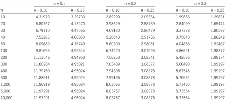
2.4. Numerical results

We provide numerical illustrations of the main results. We approximate the minimum initial capital of the discrete-time surplus process (1.2) by using Theorem 2.8 in the case of {X_n, n ≥ 1} a sequence of i.i.d. exponential distribution with intensity l= 1, by choosing model parameter combinations q= 0.10 and 0.25, i.e., c = 1.10 and c = 1.25, respectively; and

a= 0.1, 0.2, and 0.3.

Table 1 shows the approximation of MIC(a, N, c, {X_n, n ≥ 1}) with u₂₅ as mentioned in Theorem 2.8, choosing v₀= 0 and u₀= 20, and FN(u) is computed

from the recursive form (2.21).

Figure 1 shows the approximation of MIC(a, N, c, {X_n, n ≥ 1}) for the various values of a with u₂₅ as mentioned in Theorem 2.8. Here we choose v₀= 0, u₀

= 20, and parameter combinations q= 0.10, q= 0.25, i.e., c = 1.10 and c = 1.25, respectively.

3, . . . . Thus, {u_n}∞

n = 1 and {vn}∞n = 1 are convergent.

Since

uk vk u v k

k

( )

≤ − = − → → ∞

0 0 0 2 0 as ,

then there exists u* ∈ [v₀, u₀] such that

u v u

k→ ∞ k = k→ ∞ k = ∗

lim lim : . (2.27)

Since FN(u) is decreasing and FN(vk) > a for all

k= 1, 2, 3, . . . , then FN(u) > a for all u < u*. Since

F_N(u) is right continuous and F_N(u_k) ≤a for all k = 1, 2, 3, . . . , then

u u

N

( )

_k N( )k

Φ * =lim_{→ ∞}Φ ≤ α. (2.28)

Therefore,

u* MIC , , ,=

(

α N c X n

{

n, ≥1 .

}

)

(2.29)

For each k = 0, 1, 2, . . . , we have v_k≤ u* ≤ u_k. This implies that

Table 1. Minimum initial capital MIC (a, N, c, {Xn, n >– 1}) in the discrete-time surplus process with exponential claims (l = 1)

a= 0.1 a= 0.2 a= 0.3

N q= 0.10 q= 0.25 q= 0.10 q= 0.25 q= 0.10 q= 0.25

10 4.31979 3.39733 2.89299 2.09364 1.99866 1.29821

20 5.80757 4.13270 3.98629 2.58739 2.84099 1.65474

30 6.79110 4.47565 4.69130 2.80479 3.37378 1.80597

40 7.52286 4.66050 5.20540 2.91736 3.75643 1.88242

50 8.09889 4.76749 5.60309 2.98061 4.04866 1.92467

100 9.81693 4.92644 6.74520 3.07093 4.86621 1.98377

200 11.13546 4.94953 7.56253 3.08341 5.42576 1.99174

300 11.60284 4.95021 7.83409 3.08377 5.60493 1.99197

400 11.79769 4.95024 7.94308 3.08378 5.67545 1.99197

500 11.88611 4.95024 7.99136 3.08378 5.70634 1.99197

1,000 11.96919 4.95024 8.03565 3.08378 5.73435 1.99197

5,000 11.97291 4.95024 8.03757 3.08378 5.73554 1.99197

References

Dickson, D. C. M., Insurance Risk and Ruin. New York: Cam-bridge University Press, 2005.

Li, S., “On a Class of Discrete Time Renewal Risk Models,” Scandinavian Actuarial Journal 2005a(4), pp. 241–260. Li, S., “Distributions of the Surplus before Ruin, the Deficit at Ruin

and the Claim Causing Ruin in a Class of Discrete Time Risk Model,” Scandinavian Actuarial Journal 2005b (2), pp. 271–284. Pavlova, K. P., and G. E. Willmot, “The Discrete Stationary

Renewal Risk Model and the Gerber-Shiu Discounted Pen-alty Function,” Insurance: Mathematics and Economics 35(2): 2004, pp. 267–277.

Figure 1. Minimum initial capital MIC(a, N, c,

{Xn, n

>

– 1}) in the discrete-time surplus process

with exponential claims (l = 1, N = 100)

0 0.1 0.2 0.3 0.4 0.5 0.6 0.7 0.8

0 2 4 6 8 10 12 14 16 18

u∗

α

Minimum Initial Capital

u

∗