DOI 10.1007/s10115-007-0114-2 S U RV E Y PA P E R
Top 10 algorithms in data mining
Xindong Wu ·Vipin Kumar · J. Ross Quinlan· Joydeep Ghosh ·Qiang Yang · Hiroshi Motoda · Geoffrey J. McLachlan · Angus Ng· Bing Liu · Philip S. Yu· Zhi-Hua Zhou ·Michael Steinbach ·David J. Hand ·Dan Steinberg
Received: 9 July 2007 / Revised: 28 September 2007 / Accepted: 8 October 2007 Published online: 4 December 2007
© Springer-Verlag London Limited 2007
Abstract This paper presents the top 10 data mining algorithms identified by the IEEE International Conference on Data Mining (ICDM) in December 2006: C4.5, k-Means, SVM, Apriori, EM, PageRank, AdaBoost, kNN, Naive Bayes, and CART. These top 10 algorithms are among the most influential data mining algorithms in the research community. With each algorithm, we provide a description of the algorithm, discuss the impact of the algorithm, and review current and further research on the algorithm. These 10 algorithms cover classification,
X. Wu (
B
)Department of Computer Science, University of Vermont, Burlington, VT, USA e-mail: [email protected]
V. Kumar
Department of Computer Science and Engineering, University of Minnesota, Minneapolis, MN, USA e-mail: [email protected]
J. Ross Quinlan
Rulequest Research Pty Ltd, St Ives, NSW, Australia e-mail: [email protected] J. Ghosh
Department of Electrical and Computer Engineering, University of Texas at Austin, Austin, TX 78712, USA e-mail: [email protected]
Q. Yang
Department of Computer Science,
Hong Kong University of Science and Technology, Honkong, China
e-mail: [email protected] H. Motoda
AFOSR/AOARD and Osaka University,
7-23-17 Roppongi, Minato-ku, Tokyo 106-0032, Japan e-mail: [email protected]
clustering, statistical learning, association analysis, and link mining, which are all among the most important topics in data mining research and development.
0 Introduction
In an effort to identify some of the most influential algorithms that have been widely used in the data mining community, the IEEE International Conference on Data Mining (ICDM,
http://www.cs.uvm.edu/~icdm/) identified the top 10 algorithms in data mining for presen-tation at ICDM ’06 in Hong Kong.
As the first step in the identification process, in September 2006 we invited the ACM KDD Innovation Award and IEEE ICDM Research Contributions Award winners to each nomi-nate up to 10 best-known algorithms in data mining. All except one in this distinguished set of award winners responded to our invitation. We asked each nomination to provide the following information: (a) the algorithm name, (b) a brief justification, and (c) a representa-tive publication reference. We also advised that each nominated algorithm should have been widely cited and used by other researchers in the field, and the nominations from each nomi-nator as a group should have a reasonable representation of the different areas in data mining.
G. J. McLachlan
Department of Mathematics,
The University of Queensland, Brisbane, Australia e-mail: [email protected]
A. Ng
School of Medicine, Griffith University, Brisbane, Australia
B. Liu
Department of Computer Science,
University of Illinois at Chicago, Chicago, IL 60607, USA P. S. Yu
IBM T. J. Watson Research Center, Hawthorne, NY 10532, USA e-mail: [email protected] Z.-H. Zhou
National Key Laboratory for Novel Software Technology, Nanjing University, Nanjing 210093, China
e-mail: [email protected] M. Steinbach
Department of Computer Science and Engineering, University of Minnesota, Minneapolis, MN 55455, USA e-mail: [email protected]
D. J. Hand
Department of Mathematics, Imperial College, London, UK e-mail: [email protected] D. Steinberg
Salford Systems,
San Diego, CA 92123, USA e-mail: [email protected]
After the nominations in Step 1, we verified each nomination for its citations on Google Scholar in late October 2006, and removed those nominations that did not have at least 50 citations. All remaining (18) nominations were then organized in 10 topics: association anal-ysis, classification, clustering, statistical learning, bagging and boosting, sequential patterns, integrated mining, rough sets, link mining, and graph mining. For some of these 18 algorithms such as k-means, the representative publication was not necessarily the original paper that introduced the algorithm, but a recent paper that highlights the importance of the technique. These representative publications are available at the ICDM website (http://www.cs.uvm. edu/~icdm/algorithms/CandidateList.shtml).
In the third step of the identification process, we had a wider involvement of the research community. We invited the Program Committee members of KDD-06 (the 2006 ACM SIG-KDD International Conference on Knowledge Discovery and Data Mining), ICDM ’06 (the 2006 IEEE International Conference on Data Mining), and SDM ’06 (the 2006 SIAM Inter-national Conference on Data Mining), as well as the ACM KDD Innovation Award and IEEE ICDM Research Contributions Award winners to each vote for up to 10 well-known algo-rithms from the 18-algorithm candidate list. The voting results of this step were presented at the ICDM ’06 panel on Top 10 Algorithms in Data Mining.
At the ICDM ’06 panel of December 21, 2006, we also took an open vote with all 145 attendees on the top 10 algorithms from the above 18-algorithm candidate list, and the top 10 algorithms from this open vote were the same as the voting results from the above third step. The 3-hour panel was organized as the last session of the ICDM ’06 conference, in parallel with 7 paper presentation sessions of the Web Intelligence (WI ’06) and Intelligent Agent Technology (IAT ’06) conferences at the same location, and attracting 145 participants to this panel clearly showed that the panel was a great success.
1 C4.5 and beyond
1.1 Introduction
Systems that construct classifiers are one of the commonly used tools in data mining. Such systems take as input a collection of cases, each belonging to one of a small number of classes and described by its values for a fixed set of attributes, and output a classifier that can accurately predict the class to which a new case belongs.
These notes describe C4.5 [64], a descendant of CLS [41] and ID3 [62]. Like CLS and ID3, C4.5 generates classifiers expressed as decision trees, but it can also construct clas-sifiers in more comprehensible ruleset form. We will outline the algorithms employed in C4.5, highlight some changes in its successor See5/C5.0, and conclude with a couple of open research issues.
1.2 Decision trees
Given a set S of cases, C4.5 first grows an initial tree using the divide-and-conquer algorithm as follows:
• If all the cases in S belong to the same class or S is small, the tree is a leaf labeled with the most frequent class in S.
• Otherwise, choose a test based on a single attribute with two or more outcomes. Make this test the root of the tree with one branch for each outcome of the test, partition S into corresponding subsets S1, S2, . . .according to the outcome for each case, and apply the same procedure recursively to each subset.
There are usually many tests that could be chosen in this last step. C4.5 uses two heuristic criteria to rank possible tests: information gain, which minimizes the total entropy of the subsets {Si} (but is heavily biased towards tests with numerous outcomes), and the default
gain ratio that divides information gain by the information provided by the test outcomes. Attributes can be either numeric or nominal and this determines the format of the test outcomes. For a numeric attribute A they are { A≤h,A>h} where the threshold h is found by sorting S on the values of A and choosing the split between successive values that max-imizes the criterion above. An attribute A with discrete values has by default one outcome for each value, but an option allows the values to be grouped into two or more subsets with one outcome for each subset.
The initial tree is then pruned to avoid overfitting. The pruning algorithm is based on a pessimistic estimate of the error rate associated with a set of N cases, E of which do not belong to the most frequent class. Instead of E/N , C4.5 determines the upper limit of the binomial probability when E events have been observed in N trials, using a user-specified confidence whose default value is 0.25.
Pruning is carried out from the leaves to the root. The estimated error at a leaf with N cases and E errors is N times the pessimistic error rate as above. For a subtree, C4.5 adds the estimated errors of the branches and compares this to the estimated error if the subtree is replaced by a leaf; if the latter is no higher than the former, the subtree is pruned. Similarly, C4.5 checks the estimated error if the subtree is replaced by one of its branches and when this appears beneficial the tree is modified accordingly. The pruning process is completed in one pass through the tree.
C4.5’s tree-construction algorithm differs in several respects from CART [9], for instance: • Tests in CART are always binary, but C4.5 allows two or more outcomes.
• CART uses the Gini diversity index to rank tests, whereas C4.5 uses information-based criteria.
• CART prunes trees using a cost-complexity model whose parameters are estimated by cross-validation; C4.5 uses a single-pass algorithm derived from binomial confidence limits.
• This brief discussion has not mentioned what happens when some of a case’s values are unknown. CART looks for surrogate tests that approximate the outcomes when the tested attribute has an unknown value, but C4.5 apportions the case probabilistically among the outcomes.
1.3 Ruleset classifiers
Complex decision trees can be difficult to understand, for instance because information about one class is usually distributed throughout the tree. C4.5 introduced an alternative formalism consisting of a list of rules of the form “if A and B and C and ... then class X”, where rules for each class are grouped together. A case is classified by finding the first rule whose conditions are satisfied by the case; if no rule is satisfied, the case is assigned to a default class.
C4.5 rulesets are formed from the initial (unpruned) decision tree. Each path from the root of the tree to a leaf becomes a prototype rule whose conditions are the outcomes along the path and whose class is the label of the leaf. This rule is then simplified by determining the effect of discarding each condition in turn. Dropping a condition may increase the number N of cases covered by the rule, and also the number E of cases that do not belong to the class nominated by the rule, and may lower the pessimistic error rate determined as above. A hill-climbing algorithm is used to drop conditions until the lowest pessimistic error rate is found.
To complete the process, a subset of simplified rules is selected for each class in turn. These class subsets are ordered to minimize the error on the training cases and a default class is chosen. The final ruleset usually has far fewer rules than the number of leaves on the pruned decision tree.
The principal disadvantage of C4.5’s rulesets is the amount of CPU time and memory that they require. In one experiment, samples ranging from 10,000 to 100,000 cases were drawn from a large dataset. For decision trees, moving from 10 to 100K cases increased CPU time on a PC from 1.4 to 61 s, a factor of 44. The time required for rulesets, however, increased from 32 to 9,715 s, a factor of 300.
1.4 See5/C5.0
C4.5 was superseded in 1997 by a commercial system See5/C5.0 (or C5.0 for short). The changes encompass new capabilities as well as much-improved efficiency, and include: • A variant of boosting [24], which constructs an ensemble of classifiers that are then voted
to give a final classification. Boosting often leads to a dramatic improvement in predictive accuracy.
• New data types (e.g., dates), “not applicable” values, variable misclassification costs, and mechanisms to pre-filter attributes.
• Unordered rulesets—when a case is classified, all applicable rules are found and voted. This improves both the interpretability of rulesets and their predictive accuracy. • Greatly improved scalability of both decision trees and (particularly) rulesets.
Scalabili-ty is enhanced by multi-threading; C5.0 can take advantage of computers with multiple CPUs and/or cores.
More details are available fromhttp://rulequest.com/see5-comparison.html.
1.5 Research issues
We have frequently heard colleagues express the view that decision trees are a “solved prob-lem.” We do not agree with this proposition and will close with a couple of open research problems.
Stable trees. It is well known that the error rate of a tree on the cases from which it was con-structed (the resubstitution error rate) is much lower than the error rate on unseen cases (the predictive error rate). For example, on a well-known letter recognition dataset with 20,000 cases, the resubstitution error rate for C4.5 is 4%, but the error rate from a leave-one-out (20,000-fold) cross-validation is 11.7%. As this demonstrates, leaving out a single case from 20,000 often affects the tree that is constructed!
Suppose now that we could develop a non-trivial tree-construction algorithm that was hardly ever affected by omitting a single case. For such stable trees, the resubstitution error rate should approximate the leave-one-out cross-validated error rate, suggesting that the tree is of the “right” size.
Decomposing complex trees. Ensemble classifiers, whether generated by boosting, bag-ging, weight randomization, or other techniques, usually offer improved predictive accuracy. Now, given a small number of decision trees, it is possible to generate a single (very complex) tree that is exactly equivalent to voting the original trees, but can we go the other way? That is, can a complex tree be broken down to a small collection of simple trees that, when voted together, give the same result as the complex tree? Such decomposition would be of great help in producing comprehensible decision trees.
C4.5 Acknowledgments
Research on C4.5 was funded for many years by the Australian Research Council.
C4.5 is freely available for research and teaching, and source can be downloaded from
http://rulequest.com/Personal/c4.5r8.tar.gz.
2 The k-means algorithm
2.1 The algorithm
Thek-meansalgorithm is a simple iterative method to partition a given dataset into a user-specified number of clusters, k. This algorithm has been discovered by several researchers across different disciplines, most notably Lloyd (1957, 1982) [53], Forgey (1965), Friedman and Rubin (1967), and McQueen (1967). A detailed history ofk-meansalongwith descrip-tions of several variadescrip-tions are given in [43]. Gray and Neuhoff [34] provide a nice historical background fork-meansplaced in the larger context of hill-climbing algorithms.
The algorithm operates on a set of d-dimensional vectors, D= {xi|i=1, . . . ,N}, where
xi∈ d denotes the i th data point. The algorithm is initialized by picking k points ind as
the initial k cluster representatives or “centroids”. Techniques for selecting these initial seeds include sampling at random from the dataset, setting them as the solution of clustering a small subset of the data or perturbing the global mean of the data k times. Then the algorithm iterates between two steps till convergence:
Step 1: Data Assignment. Each data point is assigned to its closest centroid, with ties broken arbitrarily. This results in a partitioning of the data.
Step 2: Relocation of “means”. Each cluster representative is relocated to the center (mean) of all data points assigned to it. If the data points come with a probability measure (weights), then the relocation is to the expectations (weighted mean) of the data partitions.
The algorithm converges when the assignments (and hence the cjvalues) no longer change.
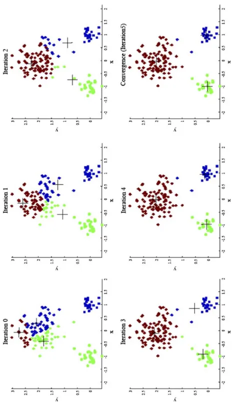
The algorithm execution is visually depicted in Fig.1. Note that each iteration needs N×k comparisons, which determines the time complexity of one iteration. The number of itera-tions required for convergence varies and may depend on N , but as a first cut, this algorithm can be considered linear in the dataset size.
One issue to resolve is how to quantify “closest” in the assignment step. The default measure of closeness is the Euclidean distance, in which case one can readily show that the non-negative cost function,
N
i=1
argmin
j
||xi−cj||22
(1)
will decrease whenever there is a change in the assignment or the relocation steps, and hence convergence is guaranteed in a finite number of iterations. The greedy-descent nature of
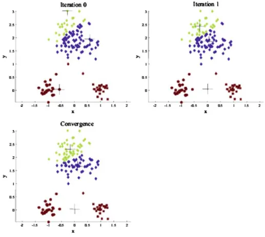
k-meanson a non-convex cost also implies that the convergence is only to a local optimum, and indeed the algorithm is typically quite sensitive to the initial centroid locations. Figure21
illustrates how a poorer result is obtained for the same dataset as in Fig.1for a different choice of the three initial centroids. The local minima problem can be countered to some 1Figures1and2are taken from the slides for the book, Introduction to Data Mining, Tan, Kumar, Steinbach, 2006.
Fig. 1 Changes in cluster representative locations (indicated by ‘+’ signs) and data assignments (indicated by color) during an execution of thek-meansalgorithm
Fig. 2 Effect of an inferior initialization on thek-meansresults
extent by running the algorithm multiple times with different initial centroids, or by doing limited local search about the converged solution.
2.2 Limitations
In addition to being sensitive to initialization, thek-meansalgorithm suffers from several other problems. First, observe thatk-meansis a limiting case of fitting data by a mixture of k Gaussians with identical, isotropic covariance matrices (=σ2I), when the soft assign-ments of data points to mixture components are hardened to allocate each data point solely to the most likely component. So, it will falter whenever the data is not well described by reasonably separated spherical balls, for example, if there are non-covex shaped clusters in the data. This problem may be alleviated by rescaling the data to “whiten” it before clustering, or by using a different distance measure that is more appropriate for the dataset. For example, information-theoretic clustering uses the KL-divergence to measure the distance between two data points representing two discrete probability distributions. It has been recently shown that if one measures distance by selecting any member of a very large class of divergences called Bregman divergences during the assignment step and makes no other changes, the essential properties ofk-means, including guaranteed convergence, linear separation boundaries and scalability, are retained [3]. This result makesk-meanseffective for a much larger class of datasets so long as an appropriate divergence is used.
k-meanscan be paired with another algorithm to describe non-convex clusters. One first clusters the data into a large number of groups usingk-means. These groups are then agglomerated into larger clusters using single link hierarchical clustering, which can detect complex shapes. This approach also makes the solution less sensitive to initialization, and since the hierarchical method provides results at multiple resolutions, one does not need to pre-specify k either.
The cost of the optimal solution decreases with increasing k till it hits zero when the number of clusters equals the number of distinct data-points. This makes it more difficult to (a) directly compare solutions with different numbers of clusters and (b) to find the opti-mum value of k. If the desired k is not known in advance, one will typically runk-means
with different values of k, and then use a suitable criterion to select one of the results. For example, SAS uses the cube-clustering-criterion, while X-means adds a complexity term (which increases with k) to the original cost function (Eq.1) and then identifies the k which minimizes this adjusted cost. Alternatively, one can progressively increase the number of clusters, in conjunction with a suitable stopping criterion. Bisectingk-means[73] achieves this by first putting all the data into a single cluster, and then recursively splitting the least compact cluster into two using 2-means. The celebrated LBG algorithm [34] used for vector quantization doubles the number of clusters till a suitable code-book size is obtained. Both these approaches thus alleviate the need to know k beforehand.
The algorithm is also sensitive to the presence of outliers, since “mean” is not a robust statistic. A preprocessing step to remove outliers can be helpful. Post-processing the results, for example to eliminate small clusters, or to merge close clusters into a large cluster, is also desirable. Ball and Hall’s ISODATA algorithm from 1967 effectively used both pre- and post-processing onk-means.
2.3 Generalizations and connections
As mentioned earlier,k-meansis closely related to fitting a mixture of k isotropic Gaussians to the data. Moreover, the generalization of the distance measure to all Bregman divergences is related to fitting the data with a mixture of k components from the exponential family of distributions. Another broad generalization is to view the “means” as probabilistic models instead of points in Rd. Here, in the assignment step, each data point is assigned to the most likely model to have generated it. In the “relocation” step, the model parameters are updated to best fit the assigned datasets. Such model-basedk-meansallow one to cater to more complex data, e.g. sequences described by Hidden Markov models.
One can also “kernelize”k-means[19]. Though boundaries between clusters are still linear in the implicit high-dimensional space, they can become non-linear when projected back to the original space, thus allowing kernelk-meansto deal with more complex clus-ters. Dhillon et al. [19] have shown a close connection between kernelk-meansand spectral clustering. The K-medoid algorithm is similar tok-meansexcept that the centroids have to belong to the data set being clustered. Fuzzy c-means is also similar, except that it computes fuzzy membership functions for each clusters rather than a hard one.
Despite its drawbacks,k-meansremains the most widely used partitional clustering algorithm in practice. The algorithm is simple, easily understandable and reasonably scal-able, and can be easily modified to deal with streaming data. To deal with very large datasets, substantial effort has also gone into further speeding upk-means, most notably by using kd-trees or exploiting the triangular inequality to avoid comparing each data point with all the centroids during the assignment step. Continual improvements and generalizations of the
basic algorithm have ensured its continued relevance and gradually increased its effectiveness as well.
3 Support vector machines
In today’s machine learning applications, support vector machines (SVM) [83] are consid-ered a must try—it offers one of the most robust and accurate methods among all well-known algorithms. It has a sound theoretical foundation, requires only a dozen examples for training, and is insensitive to the number of dimensions. In addition, efficient methods for training SVM are also being developed at a fast pace.
In a two-class learning task, the aim of SVM is to find the best classification function to distinguish between members of the two classes in the training data. The metric for the concept of the “best” classification function can be realized geometrically. For a linearly sep-arable dataset, a linear classification function corresponds to a separating hyperplane f(x) that passes through the middle of the two classes, separating the two. Once this function is determined, new data instance xncan be classified by simply testing the sign of the function
f(xn); xnbelongs to the positive class if f(xn) >0.
Because there are many such linear hyperplanes, what SVM additionally guarantee is that the best such function is found by maximizing the margin between the two classes. Intui-tively, the margin is defined as the amount of space, or separation between the two classes as defined by the hyperplane. Geometrically, the margin corresponds to the shortest distance between the closest data points to a point on the hyperplane. Having this geometric definition allows us to explore how to maximize the margin, so that even though there are an infinite number of hyperplanes, only a few qualify as the solution to SVM.
The reason why SVM insists on finding the maximum margin hyperplanes is that it offers the best generalization ability. It allows not only the best classification performance (e.g., accuracy) on the training data, but also leaves much room for the correct classification of the future data. To ensure that the maximum margin hyperplanes are actually found, an SVM classifier attempts to maximize the following function with respect tow and b:
LP=
1
2 w −
t
i=1
αiyi(w · xi+b)+
t
i=1
αi (2)
where t is the number of training examples, andαi,i=1, . . . ,t, are non-negative numbers
such that the derivatives of LPwith respect toαi are zero.αi are the Lagrange multipliers
and LP is called the Lagrangian. In this equation, the vectorsw and constant b define the
hyperplane.
There are several important questions and related extensions on the above basic formula-tion of support vector machines. We list these quesformula-tions and extensions below.
1. Can we understand the meaning of the SVM through a solid theoretical foundation? 2. Can we extend the SVM formulation to handle cases where we allow errors to exist,
when even the best hyperplane must admit some errors on the training data?
3. Can we extend the SVM formulation so that it works in situations where the training data are not linearly separable?
4. Can we extend the SVM formulation so that the task is to predict numerical values or to rank the instances in the likelihood of being a positive class member, rather than classification?
5. Can we scale up the algorithm for finding the maximum margin hyperplanes to thousands and millions of instances?
Question 1 Can we understand the meaning of the SVM through a solid theoretical foun-dation?
Several important theoretical results exist to answer this question.
A learning machine, such as the SVM, can be modeled as a function class based on some parametersα. Different function classes can have different capacity in learning, which is represented by a parameter h known as the VC dimension [83]. The VC dimension measures the maximum number of training examples where the function class can still be used to learn perfectly, by obtaining zero error rates on the training data, for any assignment of class labels on these points. It can be proven that the actual error on the future data is bounded by a sum of two terms. The first term is the training error, and the second term if proportional to the square root of the VC dimension h. Thus, if we can minimize h, we can minimize the future error, as long as we also minimize the training error. In fact, the above maximum margin function learned by SVM learning algorithms is one such function. Thus, theoretically, the SVM algorithm is well founded.
Question 2 Can we extend the SVM formulation to handle cases where we allow errors to exist, when even the best hyperplane must admit some errors on the training data?
To answer this question, imagine that there are a few points of the opposite classes that cross the middle. These points represent the training error that existing even for the maximum margin hyperplanes. The “soft margin” idea is aimed at extending the SVM algorithm [83] so that the hyperplane allows a few of such noisy data to exist. In particular, introduce a slack variableξi to account for the amount of a violation of classification by the function f(xi);
ξihas a direct geometric explanation through the distance from a mistakenly classified data
instance to the hyperplane f(x). Then, the total cost introduced by the slack variables can be used to revise the original objective minimization function.
Question 3 Can we extend the SVM formulation so that it works in situations where the training data are not linearly separable?
The answer to this question depends on an observation on the objective function where the only appearances ofxiis in the form of a dot product. Thus, if we extend the dot product
xi· xjthrough a functional mapping(xi)of eachxito a different spaceHof larger and even
possibly infinite dimensions, then the equations still hold. In each equation, where we had the dot productxi· xj, we now have the dot product of the transformed vectors(xi)·(xj),
which is called a kernel function.
The kernel function can be used to define a variety of nonlinear relationship between its inputs. For example, besides linear kernel functions, you can define quadratic or exponential kernel functions. Much study in recent years have gone into the study of different kernels for SVM classification [70] and for many other statistical tests. We can also extend the above descriptions of the SVM classifiers from binary classifiers to problems that involve more than two classes. This can be done by repeatedly using one of the classes as a positive class, and the rest as the negative classes (thus, this method is known as the one-against-all method). Question 4 Can we extend the SVM formulation so that the task is to learn to approximate data using a linear function, or to rank the instances in the likelihood of being a positive class member, rather a classification?
SVM can be easily extended to perform numerical calculations. Here we discuss two such extensions. The first is to extend SVM to perform regression analysis, where the goal is to produce a linear function that can approximate that target function. Careful consideration goes into the choice of the error models; in support vector regression, or SVR, the error is defined to be zero when the difference between actual and predicted values are within a epsi-lon amount. Otherwise, the epsiepsi-lon insensitive error will grow linearly. The support vectors can then be learned through the minimization of the Lagrangian. An advantage of support vector regression is reported to be its insensitivity to outliers.
Another extension is to learn to rank elements rather than producing a classification for individual elements [39]. Ranking can be reduced to comparing pairs of instances and pro-ducing a+1 estimate if the pair is in the correct ranking order, and−1 otherwise. Thus, a way to reduce this task to SVM learning is to construct new instances for each pair of ranked instance in the training data, and to learn a hyperplane on this new training data.
This method can be applied to many areas where ranking is important, such as in document ranking in information retrieval areas.
Question 5 Can we scale up the algorithm for finding the maximum margin hyperplanes to thousands and millions of instances?
One of the initial drawbacks of SVM is its computational inefficiency. However, this prob-lem is being solved with great success. One approach is to break a large optimization probprob-lem into a series of smaller problems, where each problem only involves a couple of carefully chosen variables so that the optimization can be done efficiently. The process iterates until all the decomposed optimization problems are solved successfully. A more recent approach is to consider the problem of learning an SVM as that of finding an approximate minimum enclosing ball of a set of instances.
These instances, when mapped to an N -dimensional space, represent a core set that can be used to construct an approximation to the minimum enclosing ball. Solving the SVM learning problem on these core sets can produce a good approximation solution in very fast speed. For example, the core-vector machine [81] thus produced can learn an SVM for millions of data in seconds.
4 The Apriori algorithm
4.1 Description of the algorithm
One of the most popular data mining approaches is to find frequent itemsets from a transaction dataset and derive association rules. Finding frequent itemsets (itemsets with frequency larger than or equal to a user specified minimum support) is not trivial because of its combinatorial explosion. Once frequent itemsets are obtained, it is straightforward to generate association rules with confidence larger than or equal to a user specified minimum confidence.
Apriori is a seminal algorithm for finding frequent itemsets using candidate generation [1]. It is characterized as a level-wise complete search algorithm using anti-monotonicity of itemsets, “if an itemset is not frequent, any of its superset is never frequent”. By convention, Apriori assumes that items within a transaction or itemset are sorted in lexicographic order. Let the set of frequent itemsets of size k be Fkand their candidates be Ck. Apriori first scans
the database and searches for frequent itemsets of size 1 by accumulating the count for each item and collecting those that satisfy the minimum support requirement. It then iterates on the following three steps and extracts all the frequent itemsets.
1. Generate Ck+1, candidates of frequent itemsets of size k+1, from the frequent itemsets of size k.
2. Scan the database and calculate the support of each candidate of frequent itemsets. 3. Add those itemsets that satisfies the minimum support requirement to Fk+1.
The Apriori algorithm is shown in Fig.3. Function apriori-gen in line 3 generates Ck+1 from Fkin the following two step process:
1. Join step: Generate RK+1, the initial candidates of frequent itemsets of size k+1 by taking the union of the two frequent itemsets of size k, Pkand Qkthat have the first k−1
elements in common.
RK+1= Pk∪Qk = {i teml, . . . ,i temk−1,i temk,i temk}
Pk= {i teml,i tem2, . . . ,i temk−1,i temk}
Qk= {i teml,i tem2, . . . ,i temk−1,i temk}
where, i teml<i tem2<· · ·<i temk<i temk.
2. Prune step: Check if all the itemsets of size k in Rk+1are frequent and generate Ck+1by removing those that do not pass this requirement from Rk+1. This is because any subset of size k of Ck+1 that is not frequent cannot be a subset of a frequent itemset of size k+1.
Function subset in line 5 finds all the candidates of the frequent itemsets included in trans-action t. Apriori, then, calculates frequency only for those candidates generated this way by scanning the database.
It is evident that Apriori scans the database at most kmax+1times when the maximum size of frequent itemsets is set at kmax.
The Apriori achieves good performance by reducing the size of candidate sets (Fig.3). However, in situations with very many frequent itemsets, large itemsets, or very low min-imum support, it still suffers from the cost of generating a huge number of candidate sets
and scanning the database repeatedly to check a large set of candidate itemsets. In fact, it is necessary to generate 2100candidate itemsets to obtain frequent itemsets of size 100.
4.2 The impact of the algorithm
Many of the pattern finding algorithms such as decision tree, classification rules and clustering techniques that are frequently used in data mining have been developed in machine learning research community. Frequent pattern and association rule mining is one of the few excep-tions to this tradition. The introduction of this technique boosted data mining research and its impact is tremendous. The algorithm is quite simple and easy to implement. Experimenting with Apriori-like algorithm is the first thing that data miners try to do.
4.3 Current and further research
Since Apriori algorithm was first introduced and as experience was accumulated, there have been many attempts to devise more efficient algorithms of frequent itemset mining. Many of them share the same idea with Apriori in that they generate candidates. These include hash-based technique, partitioning, sampling and using vertical data format. Hash-based technique can reduce the size of candidate itemsets. Each itemset is hashed into a corre-sponding bucket by using an appropriate hash function. Since a bucket can contain different itemsets, if its count is less than a minimum support, these itemsets in the bucket can be removed from the candidate sets. A partitioning can be used to divide the entire mining prob-lem into n smaller probprob-lems. The dataset is divided into n non-overlapping partitions such that each partition fits into main memory and each partition is mined separately. Since any itemset that is potentially frequent with respect to the entire dataset must occur as a frequent itemset in at least one of the partitions, all the frequent itemsets found this way are candidates, which can be checked by accessing the entire dataset only once. Sampling is simply to mine a random sampled small subset of the entire data. Since there is no guarantee that we can find all the frequent itemsets, normal practice is to use a lower support threshold. Trade off has to be made between accuracy and efficiency. Apriori uses a horizontal data format, i.e. frequent itemsets are associated with each transaction. Using vertical data format is to use a different format in which transaction IDs (TIDs) are associated with each itemset. With this format, mining can be performed by taking the intersection of TIDs. The support count is simply the length of the TID set for the itemset. There is no need to scan the database because TID set carries the complete information required for computing support.
The most outstanding improvement over Apriori would be a method called FP-growth (frequent pattern growth) that succeeded in eliminating candidate generation [36]. It adopts a divide and conquer strategy by (1) compressing the database representing frequent items into a structure called FP-tree (frequent pattern tree) that retains all the essential information and (2) dividing the compressed database into a set of conditional databases, each associated with one frequent itemset and mining each one separately. It scans the database only twice. In the first scan, all the frequent items and their support counts (frequencies) are derived and they are sorted in the order of descending support count in each transaction. In the second scan, items in each transaction are merged into a prefix tree and items (nodes) that appear in common in different transactions are counted. Each node is associated with an item and its count. Nodes with the same label are linked by a pointer called node-link. Since items are sorted in the descending order of frequency, nodes closer to the root of the prefix tree are shared by more transactions, thus resulting in a very compact representation that stores all the necessary information. Pattern growth algorithm works on FP-tree by choosing an
item in the order of increasing frequency and extracting frequent itemsets that contain the chosen item by recursively calling itself on the conditional FP-tree. FP-growth is an order of magnitude faster than the original Apriori algorithm.
There are several other dimensions regarding the extensions of frequent pattern mining. The major ones include the followings: (1) incorporating taxonomy in items [72]: Use of taxonomy makes it possible to extract frequent itemsets that are expressed by higher concepts even when use of the base level concepts produces only infrequent itemsets. (2) incremental mining: In this setting, it is assumed that the database is not stationary and a new instance of transaction keeps added. The algorithm in [12] updates the frequent itemsets without restarting from scratch. (3) using numeric valuable for item: When the item corresponds to a continuous numeric value, current frequent itemset mining algorithm is not applicable unless the values are discretized. A method of subspace clustering can be used to obtain an optimal value interval for each item in each itemset [85]. (4) using other measures than frequency, such as information gain orχ2 value: These measures are useful in finding discriminative patterns but unfortunately do not satisfy anti-monotonicity property. However, these mea-sures have a nice property of being convex with respect to their arguments and it is possible to estimate their upperbound for supersets of a pattern and thus prune unpromising patterns efficiently. AprioriSMP uses this principle [59]. (5) using richer expressions than itemset: Many algorithms have been proposed for sequences, tree and graphs to enable mining from more complex data structure [90,42]. (6) closed itemsets: A frequent itemset is closed if it is not included in any other frequent itemsets. Thus, once the closed itemsets are found, all the frequent itemsets can be derived from them. LCM is the most efficient algorithm to find the closed itemsets [82].
5 The EM algorithm
Finite mixture distributions provide a flexible and mathematical-based approach to the mod-eling and clustering of data observed on random phenomena. We focus here on the use of normal mixture models, which can be used to cluster continuous data and to estimate the underlying density function. These mixture models can be fitted by maximum likelihood via the EM (Expectation–Maximization) algorithm.
5.1 Introduction
Finite mixture models are being increasingly used to model the distributions of a wide variety of random phenomena and to cluster data sets [57]. Here we consider their application in the context of cluster analysis.
We let the p-dimensional vector ( y=(y1, . . . ,yp)T) contain the values of p variables
measured on each of n (independent) entities to be clustered, and we let yjdenote the value of y corresponding to the j th entity ( j=1, . . . ,n). With the mixture approach to clustering, y1, . . . ,yn are assumed to be an observed random sample from mixture of a finite number,
say g, of groups in some unknown proportionsπ1, . . . , πg.
The mixture density of yjis expressed as
f(yi;)= g
i=1
where the mixing proportionsπ1, . . . , πg sum to one and the group-conditional density
fi(yj;θi)is specified up to a vectorθiof unknown parameters (i=1, . . . ,g). The vector of
all the unknown parameters is given by
=(π1, . . . , πg−1, θ1T, . . . , θgT)T,
where the superscript “T” denotes vector transpose. Using an estimate of, this approach gives a probabilistic clustering of the data into g clusters in terms of estimates of the posterior probabilities of component membership,
τi(yj, )= πi
fi(yj;θi)
f(yj;) ,
(4) whereτi(yj)is the posterior probability that yj(really the entity with observation yj) belongs
to the i th component of the mixture (i=1, . . . ,g;j =1, . . . ,n).
The parameter vectorcan be estimated by maximum likelihood. The maximum like-lihood estimate (MLE) of,ˆ, is given by an appropriate root of the likelihood equation,
∂log L()/∂=0, (5)
where
log L()=
n
j=1
log f(yj;) (6)
is the log likelihood function for. Solutions of (6) corresponding to local maximizers can be obtained via the expectation–maximization (EM) algorithm [17].
For the modeling of continuous data, the component-conditional densities are usually taken to belong to the same parametric family, for example, the normal. In this case,
fi(yj;θi)=φ(yj;µi, i), (7)
whereφ(yj;µ, )denotes the p-dimensional multivariate normal distribution with mean
vectorµand covariance matrix.
One attractive feature of adopting mixture models with elliptically symmetric compo-nents such as the normal or t densities, is that the implied clustering is invariant under affine transformations of the data (that is, under operations relating to changes in location, scale, and rotation of the data). Thus the clustering process does not depend on irrelevant factors such as the units of measurement or the orientation of the clusters in space.
5.2 Maximum likelihood estimation of normal mixtures
McLachlan and Peel [57, Chap. 3] described the E- and M-steps of the EM algorithm for the maximum likelihood (ML) estimation of multivariate normal components; see also [56]. In the EM framework for this problem, the unobservable component labels zi j are treated as
being the “missing” data, where zi jis defined to be one or zero according as yj belongs or
does not belong to the i th component of the mixture (i=1, . . . ,g;,j=1, . . . ,n). On the (k+1)th iteration of the EM algorithm, the E-step requires taking the expectation of the complete-data log likelihood logLc(), given the current estimatek for. As is
linear in the unobservable zi j, this E-step is effected by replacing the zi jby their conditional
expectation given the observed data yj, using(k). That is, zi j is replaced byτi j(k), which
current fit(k)for(i=1, . . . ,g;j=1, . . . ,n). It can be expressed as
τ(k) i j =
π(k)
i φ(yj;µ( k)
i , ( k)
i )
f(yj;(k)) .
(8) On the M-step, the updated estimates of the mixing proportionπj, the mean vectorµi, and
the covariance matrixifor the i th component are given by
π(k+1) i =
n
j=1
τ(k) i j
n, (9)
µ(k+1)
i = n
j=1
τ(k)
i j yj
n
j=1
τ(k)
i j (10)
and
(k+1) i =
n j=1τ(
k) i j (yj−µ
(k+1)
i )(yj−µ
(k+1) i )T
n j=1τ(
k) i j
. (11)
It can be seen that the M-step exists in closed form.
These E- and M-steps are alternated until the changes in the estimated parameters or the log likelihood are less than some specified threshold.
5.3 Number of clusters
We can make a choice as to an appropriate value of g by consideration of the likelihood function. In the absence of any prior information as to the number of clusters present in the data, we monitor the increase in the log likelihood function as the value of g increases.
At any stage, the choice of g=g0versus g=g1, for instance g1 =g0+1, can be made by either performing the likelihood ratio test or by using some information-based criterion, such as BIC (Bayesian information criterion). Unfortunately, regularity conditions do not hold for the likelihood ratio test statisticλto have its usual null distribution of chi-squared with degrees of freedom equal to the difference d in the number of parameters for g=g1 and g=g0components in the mixture models. One way to proceed is to use a resampling approach as in [55]. Alternatively, one can apply BIC, which leads to the selection of g=g1 over g=g0if−2 logλis greater than d log(n).
6 PageRank
6.1 Overview
PageRank [10] was presented and published by Sergey Brin and Larry Page at the Seventh International World Wide Web Conference (WWW7) in April 1998. It is a search ranking algorithm using hyperlinks on the Web. Based on the algorithm, they built the search engine Google, which has been a huge success. Now, every search engine has its own hyperlink based ranking method.
PageRank produces a static ranking of Web pages in the sense that a PageRank value is computed for each page off-line and it does not depend on search queries. The algorithm relies on the democratic nature of the Web by using its vast link structure as an indicator of an individual page’s quality. In essence, PageRank interprets a hyperlink from page x to page y as a vote, by page x, for page y. However, PageRank looks at more than just the sheer
number of votes, or links that a page receives. It also analyzes the page that casts the vote. Votes casted by pages that are themselves “important” weigh more heavily and help to make other pages more “important”. This is exactly the idea of rank prestige in social networks [86].
6.2 The algorithm
We now introduce the PageRank formula. Let us first state some main concepts in the Web context.
In-links of page i : These are the hyperlinks that point to page i from other pages. Usually, hyperlinks from the same site are not considered.
Out-links of page i : These are the hyperlinks that point out to other pages from page i . Usually, links to pages of the same site are not considered.
The following ideas based on rank prestige [86] are used to derive the PageRank algorithm: 1. A hyperlink from a page pointing to another page is an implicit conveyance of authority to the target page. Thus, the more in-links that a page i receives, the more prestige the page i has.
2. Pages that point to page i also have their own prestige scores. A page with a higher prestige score pointing to i is more important than a page with a lower prestige score pointing to i . In other words, a page is important if it is pointed to by other important pages.
According to rank prestige in social networks, the importance of page i (i ’s PageRank score) is determined by summing up the PageRank scores of all pages that point to i . Since a page may point to many other pages, its prestige score should be shared among all the pages that it points to.
To formulate the above ideas, we treat the Web as a directed graph G =(V,E), where V is the set of vertices or nodes, i.e., the set of all pages, and E is the set of directed edges in the graph, i.e., hyperlinks. Let the total number of pages on the Web be n (i.e., n= |V|). The PageRank score of the page i (denoted by P(i)) is defined by
P(i)= (j,i)∈E
P(j) Oj
, (12)
where Ojis the number of out-links of page j . Mathematically, we have a system of n linear
equations (12) with n unknowns. We can use a matrix to represent all the equations. Let P be a n-dimensional column vector of PageRank values, i.e.,
P=(P(1),P(2), . . . ,P(n))T. Let A be the adjacency matrix of our graph with
Ai j =
1
Oi if(i,j)∈E
0 otherwise (13)
We can write the system of n equations with
P=ATP. (14)
This is the characteristic equation of the eigensystem, where the solution to P is an eigenvector with the corresponding eigenvalue of 1. Since this is a circular definition, an iterative algorithm is used to solve it. It turns out that if some conditions are satisfied, 1 is
Fig. 4 The power iteration
method for PageRank PagPeRank-Iterate(G)
0←e/n
k←1
repeat
; )
1
( k-1
T
k d e dA P
P ← − +
k←k + 1; until ||Pk – Pk-1||1<ε
return Pk
the largest eigenvalue and the PageRank vector P is the principal eigenvector. A well known mathematical technique called power iteration [30] can be used to find P.
However, the problem is that Eq. (14) does not quite suffice because the Web graph does not meet the conditions. In fact, Eq. (14) can also be derived based on the Markov chain. Then some theoretical results from Markov chains can be applied. After augmenting the Web graph to satisfy the conditions, the following PageRank equation is produced:
P=(1−d)e+dATP, (15)
where e is a column vector of all 1’s. This gives us the PageRank formula for each page i : P(i)=(1−d)+d
n
j=1
Aj iP(j), (16)
which is equivalent to the formula given in the original PageRank papers [10,61]: P(i)=(1−d)+d
(j,i)∈E
P(j) Oj .
(17)
The parameter d is called the damping factor which can be set to a value between 0 and 1. d = 0.85 is used in [10,52].
The computation of PageRank values of the Web pages can be done using the power iteration method [30], which produces the principal eigenvector with the eigenvalue of 1. The algorithm is simple, and is given in Fig.1. One can start with any initial assignments of PageRank values. The iteration ends when the PageRank values do not change much or converge. In Fig.4, the iteration ends after the 1-norm of the residual vector is less than a pre-specified threshold e.
Since in Web search, we are only interested in the ranking of the pages, the actual convergence may not be necessary. Thus, fewer iterations are needed. In [10], it is reported that on a database of 322 million links the algorithm converges to an acceptable tolerance in roughly 52 iterations.
6.3 Further references on PageRank
Since PageRank was presented in [10,61], researchers have proposed many enhancements to the model, alternative models, improvements for its computation, adding the tempo-ral dimension [91], etc. The books by Liu [52] and by Langville and Meyer [49] contain in-depth analyses of PageRank and several other link-based algorithms.
7 AdaBoost
7.1 Description of the algorithm
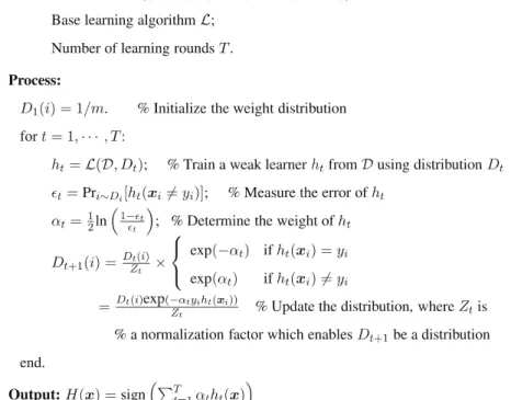
Ensemble learning [20] deals with methods which employ multiple learners to solve a prob-lem. The generalization ability of an ensemble is usually significantly better than that of a single learner, so ensemble methods are very attractive. The AdaBoost algorithm [24] pro-posed by Yoav Freund and Robert Schapire is one of the most important ensemble methods, since it has solid theoretical foundation, very accurate prediction, great simplicity (Schapire said it needs only “just 10 lines of code”), and wide and successful applications.
LetX denote the instance space andY the set of class labels. AssumeY = {−1,+1}. Given a weak or base learning algorithm and a training set{(x1,y1), (x2,y2), . . . , (xm,ym)}
where xi ∈X and yi ∈Y(i =1, . . . ,m), the AdaBoost algorithm works as follows. First,
it assigns equal weights to all the training examples(xi,yi)(i ∈ {1, . . . ,m}). Denote the
distribution of the weights at the t-th learning round as Dt. From the training set and Dt
the algorithm generates a weak or base learner ht : X →Y by calling the base learning
algorithm. Then, it uses the training examples to test ht, and the weights of the incorrectly
classified examples will be increased. Thus, an updated weight distribution Dt+1is obtained. From the training set and Dt+1 AdaBoost generates another weak learner by calling the base learning algorithm again. Such a process is repeated for T rounds, and the final model is derived by weighted majority voting of the T weak learners, where the weights of the learners are determined during the training process. In practice, the base learning algorithm may be a learning algorithm which can use weighted training examples directly; otherwise the weights can be exploited by sampling the training examples according to the weight distribution Dt.
The pseudo-code of AdaBoost is shown in Fig.5.
In order to deal with multi-class problems, Freund and Schapire presented the Ada-Boost.M1 algorithm [24] which requires that the weak learners are strong enough even on hard distributions generated during the AdaBoost process. Another popular multi-class version of AdaBoost is AdaBoost.MH [69] which works by decomposing multi-class task to a series of binary tasks. AdaBoost algorithms for dealing with regression problems have also been studied. Since many variants of AdaBoost have been developed during the past decade, Boosting has become the most important “family” of ensemble methods.
7.2 Impact of the algorithm
As mentioned in Sect.7.1, AdaBoost is one of the most important ensemble methods, so it is not strange that its high impact can be observed here and there. In this short article we only briefly introduce two issues, one theoretical and the other applied.
In 1988, Kearns and Valiant posed an interesting question, i.e., whether a weak learning algorithm that performs just slightly better than random guess could be “boosted” into an arbitrarily accurate strong learning algorithm. In other words, whether two complexity clas-ses, weakly learnable and strongly learnable problems, are equal. Schapire [67] found that the answer to the question is “yes”, and the proof he gave is a construction, which is the first Boosting algorithm. So, it is evident that AdaBoost was born with theoretical significance. AdaBoost has given rise to abundant research on theoretical aspects of ensemble methods, which can be easily found in machine learning and statistics literature. It is worth mentioning that for their AdaBoost paper [24], Schapire and Freund won the Godel Prize, which is one of the most prestigious awards in theoretical computer science, in the year of 2003.
Fig. 5 The AdaBoost algorithm
AdaBoost and its variants have been applied to diverse domains with great success. For example, Viola and Jones [84] combined AdaBoost with a cascade process for face detection. They regarded rectangular features as weak learners, and by using AdaBoost to weight the weak learners, they got very intuitive features for face detection. In order to get high accuracy as well as high efficiency, they used a cascade process (which is beyond the scope of this article). As the result, they reported a very strong face detector: On a 466 MHz machine, face detection on a 384×288 image cost only 0.067 seconds, which is 15 times faster than state-of-the-art face detectors at that time but with comparable accuracy. This face detector has been recognized as one of the most exciting breakthroughs in computer vision (in par-ticular, face detection) during the past decade. It is not strange that “Boosting” has become a buzzword in computer vision and many other application areas.
7.3 Further research
Many interesting topics worth further studying. Here we only discuss on one theoretical topic and one applied topic.
Many empirical study show that AdaBoost often does not overfit, i.e., the test error of AdaBoost often tends to decrease even after the training error is zero. Many researchers have studied this and several theoretical explanations have been given, e.g. [38]. Schapire et al. [68] presented a margin-based explanation. They argued that AdaBoost is able to increase the margins even after the training error is zero, and thus it does not overfit even after a large num-ber of rounds. However, Breiman [8] indicated that larger margin does not necessarily mean
better generalization, which seriously challenged the margin-based explanation. Recently, Reyzin and Schapire [65] found that Breiman considered minimum margin instead of aver-age or median margin, which suggests that the margin-based explanation still has chance to survive. If this explanation succeeds, a strong connection between AdaBoost and SVM could be found. It is obvious that this topic is well worth studying.
Many real-world applications are born with high dimensionality, i.e., with a large amount of input features. There are two paradigms that can help us to deal with such kind of data, i.e., dimension reduction and feature selection. Dimension reduction methods are usually based on mathematical projections, which attempt to transform the original features into an appro-priate feature space. After dimension reduction, the original meaning of the features is usually lost. Feature selection methods directly select some original features to use, and therefore they can preserve the original meaning of the features, which is very desirable in many appli-cations. However, feature selection methods are usually based on heuristics, lacking solid theoretical foundation. Inspired by Viola and Jones’s work [84], we think AdaBoost could be very useful in feature selection, especially when considering that it has solid theoretical foundation. Current research mainly focus on images, yet we think general AdaBoost-based feature selection techniques are well worth studying.
8 kNN: k-nearest neighbor classification
8.1 Description of the algorithm
One of the simplest, and rather trivial classifiers is the Rote classifier, which memorizes the entire training data and performs classification only if the attributes of the test object match one of the training examples exactly. An obvious drawback of this approach is that many test records will not be classified because they do not exactly match any of the training records. A more sophisticated approach, k-nearest neighbor (kNN) classification [23,75], finds a group of k objects in the training set that are closest to the test object, and bases the assignment of a label on the predominance of a particular class in this neighborhood. There are three key elements of this approach: a set of labeled objects, e.g., a set of stored records, a distance or similarity metric to compute distance between objects, and the value of k, the number of nearest neighbors. To classify an unlabeled object, the distance of this object to the labeled objects is computed, its k-nearest neighbors are identified, and the class labels of these nearest neighbors are then used to determine the class label of the object.
Figure6provides a high-level summary of the nearest-neighbor classification method. Given a training set D and a test object x=(x,y), the algorithm computes the distance (or similarity) between z and all the training objects(x,y)∈D to determine its nearest-neighbor list, Dz. (x is the data of a training object, while y is its class. Likewise, xis the data of the
test object and yis its class.)
Once the nearest-neighbor list is obtained, the test object is classified based on the majority class of its nearest neighbors:
Majority Voting: y=argmax v
(xi,yi)∈Dz
I(v=yi), (18)
wherev is a class label, yi is the class label for the i th nearest neighbors, and I(·)is an
Input: the set of trainingobjects and test object x Process:
Compute x , x , the distance between and every object, x Select , the set of closest trainingobjects to .
Output: argmax x
Fig. 6 The k-nearest neighbor classification algorithm
8.2 Issues
There are several key issues that affect the performance of kNN. One is the choice of k. If k is too small, then the result can be sensitive to noise points. On the other hand, if k is too large, then the neighborhood may include too many points from other classes.
Another issue is the approach to combining the class labels. The simplest method is to take a majority vote, but this can be a problem if the nearest neighbors vary widely in their distance and the closer neighbors more reliably indicate the class of the object. A more sophisticated approach, which is usually much less sensitive to the choice of k, weights each object’s vote by its distance, where the weight factor is often taken to be the reciprocal of the squared distance:wi =1/d(x,xi)2. This amounts to replacing the last step of the kNN algorithm
with the following:
Distance-Weighted Voting: y=argmax v
(xi,yi)∈Dz
wi×I(v=yi). (19)
The choice of the distance measure is another important consideration. Although various measures can be used to compute the distance between two points, the most desirable distance measure is one for which a smaller distance between two objects implies a greater likelihood of having the same class. Thus, for example, if kNN is being applied to classify documents, then it may be better to use the cosine measure rather than Euclidean distance. Some distance measures can also be affected by the high dimensionality of the data. In particular, it is well known that the Euclidean distance measure become less discriminating as the number of attributes increases. Also, attributes may have to be scaled to prevent distance measures from being dominated by one of the attributes. For example, consider a data set where the height of a person varies from 1.5 to 1.8 m, the weight of a person varies from 90 to 300 lb, and the income of a person varies from $10,000 to $1,000,000. If a distance measure is used without scaling, the income attribute will dominate the computation of distance and thus, the assignment of class labels. A number of schemes have been developed that try to compute the weights of each individual attribute based upon a training set [32].
In addition, weights can be assigned to the training objects themselves. This can give more weight to highly reliable training objects, while reducing the impact of unreliable objects. The PEBLS system by by Cost and Salzberg [14] is a well known example of such an approach. KNN classifiers are lazy learners, that is, models are not built explicitly unlike eager learners (e.g., decision trees, SVM, etc.). Thus, building the model is cheap, but classifying unknown objects is relatively expensive since it requires the computation of the k-nearest neighbors of the object to be labeled. This, in general, requires computing the distance of the unlabeled object to all the objects in the labeled set, which can be expensive particularly for large training sets. A number of techniques have been developed for efficient computation
of k-nearest neighbor distance that make use of the structure in the data to avoid having to compute distance to all objects in the training set. These techniques, which are particularly applicable for low dimensional data, can help reduce the computational cost without affecting classification accuracy.
8.3 Impact
KNN classification is an easy to understand and easy to implement classification technique. Despite its simplicity, it can perform well in many situations. In particular, a well known result by Cover and Hart [15] shows that the the error of the nearest neighbor rule is bounded above by twice the Bayes error under certain reasonable assumptions. Also, the error of the general kNN method asymptotically approaches that of the Bayes error and can be used to approximate it.
KNN is particularly well suited for multi-modal classes as well as applications in which an object can have many class labels. For example, for the assignment of functions to genes based on expression profiles, some researchers found that kNN outperformed SVM, which is a much more sophisticated classification scheme [48].
8.4 Current and future research
Although the basic kNN algorithm and some of its variations, such as weighted kNN and assigning weights to objects, are relatively well known, some of the more advanced tech-niques for kNN are much less known. For example, it is typically possible to eliminate many of the stored data objects, but still retain the classification accuracy of the kNN classifier. This is known as ‘condensing’ and can greatly speed up the classification of new objects [35]. In addition, data objects can be removed to improve classification accuracy, a process known as “editing” [88]. There has also been a considerable amount of work on the application of proximity graphs (nearest neighbor graphs, minimum spanning trees, relative neighborhood graphs, Delaunay triangulations, and Gabriel graphs) to the kNN problem. Recent papers by Toussaint [79,80], which emphasize a proximity graph viewpoint, provide an overview of work addressing these three areas and indicate some remaining open problems. Other impor-tant resources include the collection of papers by Dasarathy [16] and the book by Devroye et al. [18]. Finally, a fuzzy approach to kNN can be found in the work of Bezdek [4].
9 Naive Bayes
9.1 Introduction
Given a set of objects, each of which belongs to a known class, and each of which has a known vector of variables, our aim is to construct a rule which will allow us to assign future objects to a class, given only the vectors of variables describing the future objects. Problems of this kind, called problems of supervised classification, are ubiquitous, and many methods for constructing such rules have been developed. One very important one is the naive Bayes method—also called idiot’s Bayes, simple Bayes, and independence Bayes. This method is important for several reasons. It is very easy to construct, not needing any complicated iterative parameter estimation schemes. This means it may be readily applied to huge data sets. It is easy to interpret, so users unskilled in classifier technology can understand why it is making the classification it makes. And finally, it often does surprisingly well: it may not