On Smoothing and Inference for Topic Models
Arthur Asuncion, Max Welling, Padhraic Smyth
Department of Computer Science University of California, Irvine
Irvine, CA, USA
{asuncion,welling,smyth}@ics.uci.edu
Yee Whye Teh
Gatsby Computational Neuroscience Unit University College London
London, UK [email protected]
Abstract
Latent Dirichlet analysis, or topic modeling, is a flexible latent variable framework for model-ing high-dimensional sparse count data. Various learning algorithms have been developed in re-cent years, including collapsed Gibbs sampling, variational inference, and maximum a posteriori estimation, and this variety motivates the need for careful empirical comparisons. In this paper, we highlight the close connections between these approaches. We find that the main differences are attributable to the amount of smoothing applied to the counts. When the hyperparameters are op-timized, the differences in performance among the algorithms diminish significantly. The ability of these algorithms to achieve solutions of com-parable accuracy gives us the freedom to select computationally efficient approaches. Using the insights gained from this comparative study, we show how accurate topic models can be learned in several seconds on text corpora with thousands of documents.
1
INTRODUCTION
Latent Dirichlet Allocation (LDA) [Blei et al., 2003] and Probabilistic Latent Semantic Analysis (PLSA) [Hofmann, 2001] are well-known latent variable models for high di-mensional count data, such as text data in the bag-of-words representation or images represented through fea-ture counts. Various inference techniques have been pro-posed, including collapsed Gibbs sampling (CGS) [Grif-fiths and Steyvers, 2004], variational Bayesian inference (VB) [Blei et al., 2003], collapsed variational Bayesian in-ference (CVB) [Teh et al., 2007], maximum likelihood esti-mation (ML) [Hofmann, 2001], and maximum a posteriori estimation (MAP) [Chien and Wu, 2008].
Among these algorithms, substantial performance differ-ences have been observed in practice. For instance, Blei
et al. [2003] have shown that the VB algorithm for LDA outperforms ML estimation for PLSA. Furthermore, Teh et al. [2007] have found that CVB is significantly more ac-curate than VB. But can these differences in performance really be attributed to the type of inference algorithm? In this paper, we provide convincing empirical evidence that points in a different direction, namely that the claimed differences can be explained away by the different settings of two smoothing parameters (or hyperparameters). In fact, our empirical results suggest that these inference algo-rithms have relatively similar predictive performance when the hyperparameters for each method are selected in an op-timal fashion. With hindsight, this phenomenon should not surprise us. Topic models operate in extremely high di-mensional spaces (with typically more than 10,000 dimen-sions) and, as a consequence, the “curse of dimensionality” is lurking around the corner; thus, hyperparameter settings have the potential to significantly affect the results. We show that the potential perplexity gains by careful treatment of hyperparameters are on the order of (if not greater than) the differences between different inference al-gorithms. These results caution against using generic hy-perparameter settings when comparing results across algo-rithms. This in turn raises the question as to whether newly introduced models and approximate inference algorithms have real merit, or whether the observed difference in pre-dictive performance is attributable to suboptimal settings of hyperparameters for the algorithms being compared. In performing this study, we discovered that an algorithm which suggests itself in thinking about inference algo-rithms in a unified way – but was never proposed by itself before – performs best, albeit marginally so. More impor-tantly, it happens to be the most computationally efficient algorithm as well.
In the following section, we highlight the similarities be-tween each of the algorithms. We then discuss the impor-tance of hyperparameter settings. We show accuracy re-sults, using perplexity and precision/recall metrics, for each algorithm over various text data sets. We then focus on
α
i
x
kφ
η
i
d
z
ij
θ
N
Figure 1: Graphical model for Latent Dirichlet Allocation. Boxes denote parameters, and shaded/unshaded circles de-note observed/hidden variables.
computational efficiency and provide timing results across algorithms. Finally, we discuss related work and conclude with future directions.
2
INFERENCE TECHNIQUES FOR LDA
LDA has roots in earlier statistical decomposition tech-niques, such as Latent Semantic Analysis (LSA) [Deer-wester et al., 1990] and Probabilistic Latent Semantic Anal-ysis (PLSA) [Hofmann, 2001]. Proposed as a generaliza-tion of PLSA, LDA was cast within the generative Bayesian framework to avoid some of the overfitting issues that were observed with PLSA [Blei et al., 2003]. A review of the similarities between LSA, PLSA, LDA, and other models can be found in Buntine and Jakulin [2006].We describe the LDA model and begin with general nota-tion. LDA assumes the standard bag-of-words representa-tion, whereDdocuments are each represented as a vector of counts withW components, whereW is the number of words in the vocabulary. Each documentjin the corpus is modeled as a mixture overKtopics, and each topickis a distribution over the vocabulary ofW words. Each topic,
φ·k, is drawn from a Dirichlet with parameterη, while each document’s mixture,θ·j, is sampled from a Dirichlet with parameterα1. For each tokeniin the corpus, a topic as-signmentziis sampled fromθ·di, and the specific wordxi
is drawn fromφ·zi. The generative process is below: θk,j ∼ D[α] φw,k∼ D[η] zi∼θk,di xi∼φw,zi.
In Figure 1, the graphical model for LDA is presented in a slightly unconventional fashion, as a Bayesian network whereθkjandφwkare conditional probability tables andi runs over all tokens in the corpus. Each token’s document indexdiis explicitly shown as an observed variable, in or-der to show LDA’s correspondence to the PLSA model. Exact inference (i.e. computing the posterior over the hid-den variables) for this model is intractable [Blei et al., 2003], and so a variety of approximate algorithms have been developed. If we ignore αandη and treatθkj and
φwk as parameters, we obtain the PLSA model, and max-imum likelihood (ML) estimation over θkj and φwk di-rectly corresponds to PLSA’s EM algorithm. Adding the hyperparametersαandηback in leads to MAP estimation.
1
We use symmetric Dirichlet priors for simplicity in this paper.
Treating θkj andφwk as hidden variables and factorizing the posterior distribution leads to the VB algorithm, while collapsingθkjandφwk(i.e. marginalizing over these vari-ables) leads to the CVB and CGS algorithms. In the fol-lowing subsections, we provide details for each approach.
2.1 ML ESTIMATION
The PLSA algorithm described in Hofmann [2001] can be understood as an expectation maximization algorithm for the model depicted in Figure 1. We start the derivation by writing the log-likelihood as,
ℓ=X
i
logX
zi
P(xi|zi, φ)P(zi|di, θ)
from which we derive via a standard EM derivation the up-dates (where we have left out explicit normalizations):
P(zi|xi, di)∝P(xi|zi, φ)P(zi|di, θ) (1)
φw,k∝
X
i
I[xi=w, zi=k]P(zi|xi, di) (2)
θk,j∝
X
i
I[zi=k, di=j]P(zi|xi, di). (3) These updates can be rewritten by definingγwjk =P(z=
k|x = w, d = j), Nwj the number of observations for word typewin documentj,Nwk=PjNwjγwjk,Nkj =
P
wNwjγwjk,Nk=PwNwkandNj =PkNkj,
φw,k←Nwk/Nk θk,j←Nkj/Nj. Plugging these expressions back into the expression for the posterior (1) we arrive at the update,
γwjk∝
NwkNkj
Nk
(4) where the constantNj is absorbed into the normalization. Hofmann [2001] regularizes the PLSA updates by raising the right hand side of (4) to a powerβ >0and searching for the best value ofβon a validation set.
2.2 MAP ESTIMATION
We treat φ, θas random variables from now on. We add Dirichlet priors with strengthsηforφandαforθ respec-tively. This extension was introduced as “latent Dirichlet allocation” in Blei et al. [2003].
It is possible to optimize for the MAP estimate of φ, θ. The derivation is very similar to the ML derivation in the previous section, except that we now have terms corre-sponding to the log of the Dirichlet prior which are equal to P
wk(η −1) logφwk and Pkj(α−1) logθkj. After working through the math, we derive the following update (de Freitas and Barnard [2001], Chien and Wu [2008]),
γwjk∝
(Nwk+η−1)(Nkj+α−1)
(Nk+W η−W)
where α, η > 1. Upon convergence, MAP estimates are obtained:
ˆ
φwk=
Nwk+η−1
Nk+W η−W
ˆ
θkj=
Nkj+α−1
Nj+Kα−K
. (6)
2.3 VARIATIONAL BAYES
The variational Bayesian approximation (VB) to LDA fol-lows the standard variational EM framework [Attias, 2000, Ghahramani and Beal, 2000]. We introduce a factorized (and hence approximate) variational posterior distribution:
Q(φ, θ,z) = Y
k
q(φ·,k)
Y
j
q(θ·,j)
Y
i
q(zi). Using this assumption in the variational formulation of the EM algorithm [Neal and Hinton, 1998] we readily derive the VB updates analogous to the ML updates of Eqns. 2, 3 and 1:
q(φ·,k) =D[η+N·,k], Nwk=
X
i
q(zi=k)δ(xi, w) (7)
q(θ·,j) =D[α+N·,j], Nkj =
X
i
q(zi=k)δ(di, j) (8)
q(zi)∝exp E[logφxi,zi]q(φ)E[logθzi,di]q(θ)
. (9) We can insert the expression for q(φ)at (7) and q(θ) at (8) into the update for q(z) in (9) and use the fact that
E[logXi]D(X)=ψ(Xi)−ψ(PjXj)withψ(·)being the “digamma” function. As a final observation, note that there is nothing in the free energy that would render any differ-ently the distributionsq(zi)for tokens that correspond to the same word-typewin the same documentj. Hence, we can simplify and update a single prototype of that equiva-lence class, denoted asγwjk , q(zi =k)δ(xi, w)δ(di, j) as follows,
γwjk∝
exp(ψ(Nwk+η)) exp(ψ(Nk+W η))
exp ψ(Nkj+α). (10)
We note that exp(ψ(n))≈n−0.5forn >1. SinceNwk,
Nkj, andNk are aggregations of expected counts, we ex-pect many of these counts to be greater than 1. Thus, the VB update can be approximated as follows,
γwjk≈∝
(Nwk+η−0.5)
(Nk+W η−0.5)
Nkj+α−0.5
(11) which exposes the relation to the MAP update in (5). In closing this section, we mention that the original VB algorithm derived in Blei et al. [2003] was a hybrid version between what we call VB and ML here. Although they did estimate variational posteriorsq(θ), theφwere treated as parameters and were estimated through ML.
2.4 COLLAPSED VARIATIONAL BAYES
It is possible to marginalize out the random variablesθkj andφwkfrom the joint probability distribution. Following a variational treatment, we can introduce variational pos-teriors overzvariables which is once again assumed to be factorized: Q(z) = Q
iq(zi). This collapsed variational free energy represents a strictly better bound on the (nega-tive) evidence than the original VB [Teh et al., 2007]. The derivation of the update equation for the q(zi)is slightly more complicated and involves approximations to compute intractable summations. The update is given below2:
γijk∝
Nwk¬ij+η
Nk¬ij+W η
Nkj¬ij+αexp
− V
¬ij
kj
2(Nkj¬ij+α)2
− V
¬ij
wk
2(Nwk¬ij+η)2 +
Vk¬ij
2(Nk¬ij+W η)2
. (12)
Nkj¬ij denotes the expected number of tokens in document
jassigned to topick(excluding the current token), and can be calculated as follows: Nkj¬ij =
P
i′6=iγi′jk. For CVB, there is also a variance associated with each count:Vkj¬ij =
P
i′6=iγi′jk(1−γi′jk). For further details we refer to Teh et al. [2007].
The update in (12) makes use of a second-order Taylor ex-pansion as an approximation. A further approximation can be made by using only the zeroth-order information3:
γijk∝
Nwk¬ij+η
Nk¬ij+W η
Nkj¬ij+α. (13)
We refer to this approximate algorithm as CVB0.
2.5 COLLAPSED GIBBS SAMPLING
MCMC techniques are available to LDA as well. In collapsed Gibbs sampling (CGS) [Griffiths and Steyvers, 2004],θkjandφwkare integrated out (as in CVB) and sam-pling of the topic assignments is performed sequentially in the following manner:
P(zij=k|z¬ij, xij =w)∝
Nwk¬ij+η
Nk¬ij+W η
Nkj¬ij+α.
(14)
Nwk denotes the number of word tokens of type w as-signed to topic k, Nkj is the number of tokens in docu-ment j assigned to topic k, and Nk = PwNwk. N¬ij denotes the count with tokenij removed. Note that stan-dard non-collapsed Gibbs sampling over φ,θ, and z can also be performed, but we have observed that CGS mixes more quickly in practice.
2
For convenience, we switch back to the conventional
index-ing scheme for LDA whereiruns over tokens in documentj.
3
2.6 COMPARISON OF ALGORITHMS
A comparison of update equations (5), (11), (12), (13), (14) reveals the similarities between these algorithms. All of these updates consist of a product of terms featuringNwk and Nkj as well as a denominator featuringNk. These updates resemble the Callen equations [Teh et al., 2007], which the true posterior distribution must satisfy (withZ
as the normalization constant):
P(zij =k|x) =Ep(z¬ij|x)
1
Z
(Nwk¬ij+η) (Nk¬ij+W η) N
¬ij
kj +α
.
We highlight the striking connections between the algo-rithms. Interestingly, the probabilities for CGS (14) and CVB0 (13) are exactly the same. The only difference is that CGS samples each topic assignment while CVB0 de-terministically updates a discrete distribution over topics for each token. Another way to view this connection is to imagine that CGS can sample each topic assignment zij
R times using (14) and maintain a distribution over these samples with which it can update the counts. AsR→ ∞, this distribution will be exactly (13) and this algorithm will be CVB0. The fact that algorithms like CVB0 are able to propagate the entire uncertainty in the topic distribution during each update suggests that deterministic algorithms should converge more quickly than CGS.
CVB0 and CVB are almost identical as well, the distinction being the inclusion of second-order information for CVB. The conditional distributions used in VB (11) and MAP (5) are also very similar to those used for CGS, with the main difference being the presence of offsets of up to−0.5and −1in the numerator terms for VB and MAP, respectively. Through the setting of hyperparametersαandη, these extra offsets in the numerator can be eliminated, which suggests that these algorithms can be made to perform similarly with appropriate hyperparameter settings.
Another intuition which sheds light on this phenomenon is as follows. Variational methods like VB are known to underestimate posterior variance [Wang and Titterington, 2004]. In the case of LDA this is reflected in the offset of -0.5: typical values ofφandθin the variational poste-rior tend to concentrate more mass on the high probability words and topics respectively. We can counteract this by in-crementing the hyperparameters by 0.5, which encourages more probability mass to be smoothed to all words and top-ics. Similarly, MAP offsets by -1, concentrating even more mass on high probability words and topics, and requiring even more smoothing by incrementingαandηby 1. Other subtle differences between the algorithms exist. For instance, VB subtracts only 0.5 from the denominator while MAP removes W, which suggests that VB applies more smoothing to the denominator. SinceNk is usually large, we do not expect this difference to play a large role in learn-ing. For the collapsed algorithms (CGS, CVB), the counts
Nwk,Nkj,Nkare updated after each token update. Mean-while, the standard formulations of VB and MAP update these counts only after sweeping through all the tokens. This update schedule may affect the rate of convergence [Neal and Hinton, 1998]. Another difference is that the collapsed algorithms remove the count for the current to-kenij.
As we will see in the experimental results section, the per-formance differences among these algorithms that were ob-served in previous work can be substantially reduced when the hyperparameters are optimized for each algorithm.
3
THE ROLE OF HYPERPARAMETERS
The similarities between the update equations for these al-gorithms shed light on the important role that hyperparame-ters play. Since the amount of smoothing in the updates dif-ferentiates the algorithms, it is important to have good hy-perparameter settings. In previous results [Teh et al., 2007, Welling et al., 2008b, Mukherjee and Blei, 2009], hyper-parameters for VB were set to small values likeα= 0.1,
η = 0.1, and consequently, the performance of VB was observed to be significantly suboptimal in comparison to CVB and CGS. Since VB effectively adds a discount of up to−0.5in the updates, greater values forαandηare nec-essary for VB to perform well. We discuss hyperparameter learning and the role of hyperparameters in prediction.
3.1 HYPERPARAMETER LEARNING
It is possible to learn the hyperparameters during training. One approach is to place Gamma priors on the hyperpa-rameters (η∼G[a, b],α∼G[c, d]) and use Minka’s fixed-point iterations [Minka, 2000], e.g.:
α←c−1 + ˆα
P
j
P
k[Ψ(Nkj+ ˆα)−Ψ(ˆα)]
d+KP
j[Ψ(Nj+Kαˆ)−Ψ(Kαˆ)]
.
Other ways for learning hyperparameters include Newton-Raphson and other fixed-point techniques [Wallach, 2008], as well as sampling techniques [Teh et al., 2006]. Another approach is to use a validation set and to explore various settings ofα,ηthrough grid search. We explore several of these approaches later in the paper.
3.2 PREDICTION
Hyperparameters play a role in prediction as well. Consider the update for MAP in (5) and the estimates forφwkandθkj (6) and note that the terms used in learning are the same as those used in prediction. Essentially the same can be said for the collapsed algorithms, since the following Rao-Blackwellized estimates are used, which bear resemblance to terms in the updates (14), (13):
ˆ
φwk =
Nwk+η
Nk+W η
ˆ
θkj=
Nkj+α
Nj+Kα
. (15)
In the case of VB, the expected values of the posterior Dirichlets in (7) and (8) are used in prediction, leading to
Table 1: Data sets used in experiments
NAME D W Ntrain Dtest
CRAN 979 3,763 81,773 210
KOS 3,000 6,906 410,595 215
MED 9,300 5,995 886,306 169
NIPS 1,500 12,419 1,932,365 92
NEWS 19,500 27,059 2,057,207 249
NYT 6,800 16,253 3,768,969 139
PAT 6,500 19,447 14,328,094 106
estimates forφandθof the same form as (15). However, for VB, an offset of−0.5is found in update equation (10) while it is not found in the estimates used for prediction. The knowledge that VB’s update equation contains an ef-fective offset of up to−0.5suggests the use of an alterna-tive estimate for prediction:
ˆ
φwk ∝
exp(ψ(Nwk+η)) exp(ψ(Nk+W η))
ˆ
θkj∝
exp(ψ(Nkj+α)) exp(ψ(Nj+Kα))
.
(16) Note the similarity that these estimates bear to the VB up-date (10). Essentially, the −0.5 offset is introduced into these estimates just as they are found in the update. An-other way to mimic this behavior is to use α+ 0.5 and
η + 0.5 during learning and then useαandη for predic-tion, using the estimates in (15). We find that correcting this “mismatch” between the update and the estimate re-duces the performance gap between VB and the other al-gorithms. Perhaps this phenomenon bears relationships to the observation of Wainwright [2006], who shows that it certain cases, it is beneficial to use the same algorithm for both learning and prediction, even if that algorithm is ap-proximate rather than exact.
4
EXPERIMENTS
Seven different text data sets are used to evaluate the perfor-mance of these algorithms: Cranfield-subset (CRAN), Kos (KOS), Medline-subset (MED), NIPS (NIPS), 20 News-groups (NEWS), NYT-subset (NYT), and Patent (PAT). Several of these data sets are available online at the UCI ML Repository [Asuncion and Newman, 2007]. The char-acteristics of these data sets are summarized in Table 1. Each data set is separated into a training set and a test set. We learn the model on the training set, and then we mea-sure the performance of the algorithms on the test set. We also have a separate validation set of the same size as the test set that can be used to tune the hyperparameters. To evaluate accuracy, we use perplexity, a widely-used met-ric in the topic modeling community. While perplexity is a somewhat indirect measure of predictive performance, it is nonetheless a useful characterization of the predictive qual-ity of a language model and has been shown to be well-correlated with other measures of performance such word-error rate in speech recognition [Klakow and Peters, 2002]. We also report precision/recall statistics.
0 100 200 300 400 500 1000
1200 1400 1600 1800
Perplexity
Iteration
CGS VB CVB CVB0
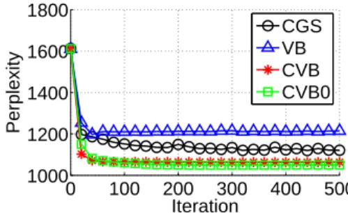
Figure 2: Convergence plot showing perplexities on MED, K=40; hyperparameters learned through Minka’s update. We describe how perplexity is computed. For each of our algorithms, we perform runs lasting 500 iterations and we obtain the estimateφˆwk at the end of each of those runs. To obtainθˆkj, one must learn the topic assignments on the first half of each document in the test set while holdingφˆwk fixed. For this fold-in procedure, we use the same learning algorithm that we used for training. Perplexity is evaluated on the second half of each document in the test set, given
ˆ
φwkandθˆjk. For CGS, one can average over multiple sam-ples (where S is the number of samsam-ples to average over):
logp(xtest) = X
jw
Njwlog
1
S X
s
X
k
ˆ
θs
kjφˆ
s
wk.
In our experiments we don’t perform averaging over sam-ples for CGS (other than in Figure 7 where we explicitly investigate averaging), both for computational reasons and to provide a fair comparison to the other algorithms. Us-ing a sUs-ingle sample from CGS is consistent with its use as an efficient stochastic “mode-finder” to find a set of inter-pretable topics for a document set.
For each experiment, we perform three different runs us-ing different initializations, and report the average of these perplexities. Usually these perplexities are similar to each other across different initializations (e.g.±10 or less).
4.1 PERPLEXITY RESULTS
In our first set of experiments, we investigate the effects of learning the hyperparameters during training using Minka’s fixed point updates. We compare CGS, VB, CVB, and CVB0 in this set of experiments and leave out MAP since Minka’s update does not apply to MAP. For each run, we initialize the hyperparameters toα= 0.5,η= 0.5and turn on Minka’s updates after 15 iterations to prevent numerical instabilities. Every other iteration, we compute perplexity on the validation set to allow us to perform early-stopping if necessary. Figure 2 shows the test perplexity as a func-tion of iterafunc-tion for each algorithm on the MED data set. These perplexity results suggest that CVB and CVB0 out-perform VB when Minka’s updates are used. The reason is because the learned hyperparameters for VB are too small and do not correct for the effective−0.5offset found in the VB update equations. Also, CGS converges more slowly than the deterministic algorithms.
0 500 1000 1500 2000 2500 3000 3500
Perplexity
CRAN KOS MED NIPS NEWS NYT PAT
CGS VB CVB CVB0
Figure 3: Perplexities achieved with hyperparameter learn-ing through Minka’s update, on various data sets, K=40.
0 50 100 150 1400
1600 1800 2000 2200
Number of Topics
Perplexity
CGS VB CVB CVB0
Figure 4: Perplexity as a function of number of topics, on NIPS, with Minka’s update enabled.
In Figure 3, we show the final perplexities achieved with hyperparameter learning (through Minka’s update), on each data set. VB performs worse on several of the data sets compared to the other algorithms. We also found that CVB0 usually learns the highest level of smoothing, fol-lowed by CVB, while Minka’s updates for VB learn small values forα,η.
In our experiments thus far, we fixed the number at topics at
K= 40. In Figure 4, we vary the number of topics from 10 to 160. In this experiment, CGS/CVB/CVB0 perform simi-larly, while VB learns less accurate solutions. Interestingly, the CVB0 perplexity at K = 160is higher than the per-plexity atK = 80. This is due to the fact that a high value for η was learned for CVB0. When we setη = 0.13(to theK = 80level), the CVB0 perplexity is 1464, matching CGS. These results suggest that learning hyperparameters during training (using Minka’s updates) does not necessar-ily lead to the optimal solution in terms of test perplexity. In the next set of experiments, we use a grid of hyperpa-rameters for each ofαandη, [0.01, 0.1, 0.25, 0.5, 0.75, 1], and we run the algorithms for each combination of hy-perparameters. We include MAP in this set of experiments, and we shift the grid to the right by 1 for MAP (since hyper-parameters less than 1 cause MAP to have negative proba-bilities). We perform grid search on the validation set, and
0 500 1000 1500 2000 2500 3000 3500
Perplexity
CRAN KOS MED NIPS NEWS
CGS VB VB (alt) CVB CVB0 MAP
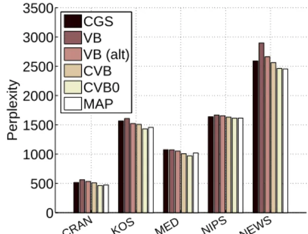
Figure 5: Perplexities achieved through grid search, K=40.
we find the best hyperparameter settings (according to val-idation set perplexity) and use the corresponding estimates for prediction. For VB, we report both the standard per-plexity calculation and the alternative calculation that was detailed previously in (16).
In Figure 5, we report the results achieved through perform-ing grid search. The differences between VB (with the al-ternative calculation) and CVB have largely vanished. This is due to the fact that we are using larger values for the hyperparameters, which allows VB to reach parity with the other algorithms. The alternative prediction scheme for VB also helps to reduce the perplexity gap, especially for the NEWS data set. Interestingly, CVB0 appears to perform slightly better than the other algorithms.
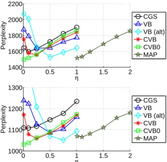
Figure 6 shows the test perplexity of each method as a function of η. It is visually apparent that VB and MAP perform better when their hyperparameter values are off-set by 0.5 and 1, respectively, relative to the other meth-ods. While this picture is not as clear-cut for every data set (since the approximate VB update holds only whenn >1), we have consistently observed that the minimum perplexi-ties achieved by VB are at hyperparameter values that are higher than the ones used by the other algorithms.
In the previous experiments, we used one sample for CGS to compute perplexity. With enough samples, CGS should be the most accurate algorithm. In Figure 7, we show the effects of averaging over 10 different samples for CGS, taken over 10 different runs, and find that CGS gains sub-stantially from averaging samples. It is also possible for other methods like CVB0 to average over their local poste-rior “modes” but we found the resulting gain is not as great. We also tested whether the algorithms would perform sim-ilarly in cases where the training set size is very small or the number of topics is very high. We ran VB and CVB with grid search on half of CRAN and achieved virtually the same perplexities. We also ran VB and CVB on CRAN withK= 100, and only found a 16-point perplexity gap.
0 0.5 1 1.5 2 1400
1600 1800 2000 2200
Perplexity
η
CGS VB VB (alt) CVB CVB0 MAP
0 0.5 1 1.5 2
1000 1100 1200 1300
Perplexity
η
CGS VB VB (alt) CVB CVB0 MAP
Figure 6: TOP: KOS, K=40. BOTTOM: MED, K=40. Per-plexity as a function ofη. We fixedαto 0.5 (1.5 for MAP). Relative to the other curves, VB and MAP curves are in effect shifted right by approximately 0.5 and 1.
0 100 200 300 400 500
1500 2000 2500
Iteration
Perplexity
CGS S=1 CVB0 S=1 CGS S=10 CVB0 S=10
Figure 7: The effect of averaging over 10 samples/modes on KOS, K=40.
To summarize our perplexity results, we juxtapose three different ways of setting hyperparameters in Figure 8, for NIPS,K = 40. The first way is to have the same arbitrary values used across all algorithms (e.g. α= 0.1,η = 0.1). The second way is to learn the hyperparameters through Minka’s update. The third way way is to find the hyperpa-rameters by grid search. For the third way, we also show the VB perplexity achieved by the alternative estimates.
4.2 PRECISION/RECALL RESULTS
We also calculated precision/recall statistics on the NEWS data set. Since each document in NEWS is associated with one of twenty newsgroups, one can label each doc-ument by its corresponding newsgroup. It is possible to use the topic model for classification and to compute pre-cision/recall statistics. In Figure 9, we show the mean area under the ROC curve (AUC) achieved by CGS, VB, CVB, and CVB0 with hyperparameter learning through Minka’s update. We also performed grid search overα,ηand found that each method was able to achieve similar statistics. For instance, on NEWS,K= 10, each algorithm achieved the
Point Minka Grid Grid (Alt) 1500
1600 1700 1800 1900
Perplexity
CGS VB CVB CVB0
Figure 8: POINT: Whenα= 0.1,η = 0.1, VB performs substantially worse than other methods. MINKA: When using Minka’s updates, the differences are less prominent. GRID: When grid search is performed, differences dimin-ish even more, especially with the alternative estimates.
0 20 40 60 80 0.65
0.7 0.75 0.8 0.85 0.9
Mean AUC
Iteration
CGS VB CVB CVB0
Figure 9: Mean AUC achieved on NEWS, K=40, with Minka’s update.
same area under the ROC curve (0.90) and mean average precision (0.14). These results are consistent with the per-plexity results in the previous section.
5
COMPUTATIONAL EFFICIENCY
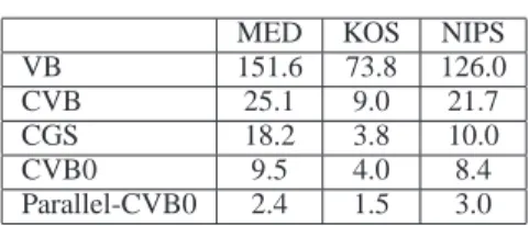
While the algorithms can give similarly accurate solutions, some of these algorithms are more efficient than others. VB contains digamma functions which are computationally ex-pensive, while CVB requires the maintenance of variance counts. Meanwhile, the stochastic nature of CGS causes it to converge more slowly than the deterministic algorithms. In practice, we advocate using CVB0 since 1) it is faster than VB/CVB given that there are no calls to digamma or variance counts to maintain; 2) it converges more quickly than CGS since it is deterministic; 3) it does not have MAP’s−1offset issue. Furthermore, our empirical results suggest that CVB0 learns models that are as good or better (predictively) than those learned by the other algorithms. These algorithms can be parallelized over multiple proces-sors as well. The updates in MAP estimation can be per-formed in parallel without affecting the fixed point since MAP is an EM algorithm [Neal and Hinton, 1998]. Since the other algorithms are very closely related to MAP there is confidence that performing parallel updates over tokens for the other algorithms would lead to good results as well.Table 2: Timing results (in seconds)
MED KOS NIPS
VB 151.6 73.8 126.0
CVB 25.1 9.0 21.7
CGS 18.2 3.8 10.0
CVB0 9.5 4.0 8.4
Parallel-CVB0 2.4 1.5 3.0
While non-collapsed algorithms such as MAP and VB can be readily parallelized, the collapsed algorithms are se-quential, and thus there has not been a theoretical basis for parallelizing CVB or CGS (although good empirical results have been achieved for approximate parallel CGS [New-man et al., 2008]). We expect that a version of CVB0 that parallelizes over tokens would converge to the same quality of solution as sequential CVB0, since CVB0 is essentially MAP but without the−1offset4.
In Table 2, we show timing results for VB, CVB, CGS, and CVB0 on MED, KOS, and NIPS, withK= 10. We record the amount of time it takes for each algorithm to pass a fixed perplexity threshold (the same for each algorithm). Since VB contains many calls to the digamma function, it is slower than the other algorithms. Meanwhile, CGS needs more iterations before it can reach the same perplex-ity, since it is stochastic. We see that CVB0 is computation-ally the fastest approach among these algorithms. We also parallelized CVB0 on a machine with 8 cores and find that a topic model with coherent topics can be learned in 1.5 seconds for KOS. These results suggest that it is feasible to learn topic models in near real-time for small corpora.
6
RELATED WORK & CONCLUSIONS
Some of these algorithms have been compared to each other in previous work. Teh et al. [2007] formulate the CVB algorithm and empirically compare it to VB, while Mukherjee and Blei [2009] theoretically analyze the differ-ences between VB and CVB and give cases for when CVB should perform better than VB. Welling et al. [2008b] also compare the algorithms and introduce a hybrid CGS/VB algorithm. In all these studies, low values ofηandαwere used for each algorithm, including VB. Our insights sug-gest that VB requires more smoothing in order to match the performance of the other algorithms.The similarities between PLSA and LDA have been noted in the past [Girolami and Kaban, 2003]. Others have uni-fied similar deterministic latent variable models [Welling et al., 2008a] and matrix factorization techniques [Singh and Gordon, 2008]. In this work, we highlight the similar-ities between various learning algorithms for LDA. While we focused on LDA and PLSA in this paper, we be-lieve that the insights gained are relevant to learning in
gen-4
If one wants convergence guarantees, one should also not
re-move the current tokenij.
eral directed graphical models with Dirichlet priors, and generalizing these results to other models is an interesting avenue to pursue in the future.
In conclusion, we have found that the update equations for these algorithms are closely connected, and that using the appropriate hyperparameters causes the performance differences between these algorithms to largely disappear. These insights suggest that hyperparameters play a large role in learning accurate topic models. Our comparative study also showed that there exist accurate and efficient learning algorithms for LDA and that these algorithms can be parallelized, allowing us to learn accurate models over thousands of documents in a matter of seconds.
Acknowledgements
This work is supported in part by NSF Awards IIS-0083489 (PS, AA), IIS-0447903 and IIS-0535278 (MW), and an NSF graduate fellowship (AA), as well as ONR grants 00014-06-1-073 (MW) and N00014-08-1-1015 (PS). PS is also supported by a Google Research Award. YWT is sup-ported by the Gatsby Charitable Foundation.
References
A. Asuncion and D. Newman. UCI machine learning repository, 2007. URL
http://www.ics.uci.edu/∼mlearn/MLRepository.html. H. Attias. A variational Bayesian framework for graphical models. In NIPS 12,
pages 209–215. MIT Press, 2000.
D. M. Blei, A. Y. Ng, and M. I. Jordan. Latent Dirichlet allocation. JMLR, 3:993– 1022, 2003.
W. Buntine and A. Jakulin. Discrete component analysis. Lecture Notes in Computer
Science, 3940:1, 2006.
J.-T. Chien and M.-S. Wu. Adaptive Bayesian latent semantic analysis. Audio,
Speech, and Language Processing, IEEE Transactions on, 16(1):198–207, 2008.
N. de Freitas and K. Barnard. Bayesian latent semantic analysis of multimedia databases. Technical Report TR-2001-15, University of British Columbia, 2001. S. Deerwester, S. Dumais, G. Furnas, T. Landauer, and R. Harshman. Indexing by
latent semantic analysis. JASIS, 41(6):391–407, 1990.
Z. Ghahramani and M. Beal. Variational inference for Bayesian mixtures of factor analysers. In NIPS 12, pages 449–455. MIT Press, 2000.
M. Girolami and A. Kaban. On an equivalence between PLSI and LDA. In SIGIR
’03, pages 433–434. ACM New York, NY, USA, 2003.
T. L. Griffiths and M. Steyvers. Finding scientific topics. PNAS, 101(Suppl 1): 5228–5235, 2004.
T. Hofmann. Unsupervised learning by probabilistic latent semantic analysis.
Ma-chine Learning, 42(1):177–196, 2001.
D. Klakow and J. Peters. Testing the correlation of word error rate and perplexity.
Speech Communication, 38(1-2):19–28, 2002.
T. Minka. Estimating a Dirichlet distribution. 2000. URL http:// research.microsoft.com/∼minka/papers/dirichlet/. I. Mukherjee and D. M. Blei. Relative performance guarantees for approximate
inference in latent Dirichlet allocation. In NIPS 21, pages 1129–1136, 2009. R. Neal and G. Hinton. A view of the EM algorithm that justifies incremental, sparse,
and other variants. Learning in graphical models, 89:355–368, 1998. D. Newman, A. Asuncion, P. Smyth, and M. Welling. Distributed inference for latent
Dirichlet allocation. In NIPS 20, pages 1081–1088. MIT Press, 2008. A. Singh and G. Gordon. A Unified View of Matrix Factorization Models. In ECML
PKDD, pages 358–373. Springer, 2008.
Y. W. Teh, M. I. Jordan, M. J. Beal, and D. M. Blei. Hierarchical Dirichlet processes.
Journal of the American Statistical Association, 101(476):1566–1581, 2006.
Y. W. Teh, D. Newman, and M. Welling. A collapsed variational Bayesian inference algorithm for latent Dirichlet allocation. In NIPS 19, pages 1353–1360. 2007. M. J. Wainwright. Estimating the ”wrong” graphical model: Benefits in the
computation-limited setting. JMLR, 7:1829–1859, 2006.
H. M. Wallach. Structured Topic Models for Language. PhD thesis, University of Cambridge, 2008.
B. Wang and D. Titterington. Convergence and asymptotic normality of variational Bayesian approximations for exponential family models with missing values. In
UAI, pages 577–584, 2004.
M. Welling, C. Chemudugunta, and N. Sutter. Deterministic latent variable models and their pitfalls. In SIAM International Conference on Data Mining, 2008a. M. Welling, Y. W. Teh, and B. Kappen. Hybrid variational/MCMC inference in