Learning Mid-Level Features For Recognition

Learning Mid-Level Features For Recognition

Y-Lan Boureau

Francis Bach

Yann LeCun

Jean Ponce

1

INRIA

Ecole Normale Sup´erieure

Courant Institute, New York University

Abstract

Many successful models for scene or object recognition transform low-level descriptors (such as Gabor filter re-sponses, or SIFT descriptors) into richer representations of intermediate complexity. This process can often be bro-ken down into two steps: (1) a coding step, which per-forms a pointwise transformation of the descriptors into a representation better adapted to the task, and (2) a pool-ing step, which summarizes the coded features over larger neighborhoods. Several combinations of coding and pool-ing schemes have been proposed in the literature. The goal of this paper is threefold. We seek to establish the rela-tive importance of each step of mid-level feature extrac-tion through a comprehensive cross evaluaextrac-tion of several types of coding modules (hard and soft vector quantization, sparse coding) and pooling schemes (by taking the aver-age, or the maximum), which obtains state-of-the-art per-formance or better on several recognition benchmarks. We show how to improve the best performing coding scheme by learning a supervised discriminative dictionary for sparse coding. We provide theoretical and empirical insight into the remarkable performance of max pooling. By teasing apart components shared by modern mid-level feature ex-tractors, our approach aims to facilitate the design of better recognition architectures.

1. Introduction

Finding good image features is critical in modern ap-proaches to category-level image classification. Many methods first extract low-level descriptors (e.g., SIFT [18] or HOG descriptors [5]) at interest point locations, or nodes in a dense grid. This paper considers the problem of com-bining these local features into a global image representa-tion suited to recognirepresenta-tion using a common classifier such as a support vector machine. Since global features built upon low-level ones typically remain close to image-level infor-mation without attempts at high-level, structured image de-scription (in terms of parts for example), we will refer to

4_{WILLOW project-team, Laboratoire d’Informatique de l’Ecole}

Nor-male Sup´erieure, ENS/INRIA/CNRS UMR 8548.

them asmid-levelfeatures.

Popular examples of mid-level features include bags of features [25], spatial pyramids [12], and the upper units of convolutional networks [13] or deep belief networks [8,23]. Extracting these mid-level features involves a sequence of interchangeable modules similar to that identified by Winder and Brown for local image descriptors [29]. In this paper, we focus on two types of modules:

• Coding: Input features are locally transformed into representations that have some desirable properties such as compactness, sparseness (i.e., most compo-nents are 0), or statistical independence. The code is typically a vector with binary (vector quantization) or continuous (HOG, sparse coding) entries, obtained by decomposing the original feature on some codebook, or dictionary.

• Spatial pooling: The codes associated with local im-age features are pooled over some imim-age neighborhood (e.g., the whole image for bags of features, a coarse grid of cells for the HOG approach to pedestrian de-tection, or a coarse hierarchy of cells for spatial pyra-mids). The codes within each cell are summarized by a single “semi-local” feature vector, common examples being the average of the codes (average pooling) or their maximum (max pooling).

The same coding and pooling modules can be plugged into various architectures. For example, average pooling is found in convolutional nets [13], bag-of-features meth-ods, and HOG descriptors; max pooling is found in convo-lutional nets [16,23], HMAX nets [24], and state-of-the-art variants of the spatial pyramid model [31]. The final global vector is formed by concatenating with suitable weights the semi-local vectors obtained for each pooling region.

High levels of performance have been reported for spe-cific pairings of coding and pooling modules (e.g., sparse coding and max pooling [31]), but it is not always clear whether the improvement can be factored into independent contributions of each module (e.g., whether the better per-formance of max pooling would generalize to systems us-ing vector quantization instead of sparse codus-ing). In this 1

work, we address this concern by presenting a comprehen-sive set of product pairings across known coding (hard and soft vector quantization, sparse coding) and pooling (aver-age and max pooling) modules. We have chosen to restrict ourselves to the spatial pyramid framework since it has al-ready been used in several comparative studies [27, 31], defining the state of the art on several benchmarks; but the insights gained within that framework should easily gen-eralize to other models (e.g., models using interest point detectors, convolutional networks, deep belief networks). Two striking results of our evaluation are that (1) sparse coding systematically outperforms the other coding mod-ules, irrespective of the pooling module, and (2) max pool-ing dramatically improves linear classification performance irrespective of the coding module, to the point that the worst-performing coding module (hard vector quantization) paired with max pooling outperforms the best coding mod-ule (sparse coding) paired with average pooling. The rest of our paper builds on these two findings. Noting that the dic-tionary used to perform sparse coding is trained to minimize reconstruction error, which might be suboptimal for classi-fication, we propose a new supervised dictionary learning algorithm. As for the superiority of max pooling in lin-ear classification, we complement the empirical finding by a theoretical analysis and new experiments. Our article thus makes three contributions:

• We systematically explore combinations of known modules appearing in the unified model presented in this paper, obtaining state-of-the-art results on two benchmarks (Sec. 3).

• We introduce a novel supervised sparse dictionary learning algorithm (Sec. 4).

• We present theoretical and experimental insights into the much better linear discrimination performance ob-tained with max pooling compared to average pooling, in a large variety of settings (Sec. 5).

2. Notation and Related Work

In this section, we introduce some notation used through-out this paper, and present coding and pooling modules pre-viously used by other authors. Let an image I be repre-sented by a set of low-level descriptors (e.g., SIFT) x_{i at}

N locations identified with their indices i = 1,· · · , N. M regions of interests are defined on the image (e.g., the

21 = 16 + 4 + 1cells of a three-level spatial pyramid), with_Nmdenoting the set of locations/indices within region m. Letf andgdenote some coding and pooling operators, respectively. The vectorz _{representing the whole image is}

obtained by sequentially coding, pooling over all regions,

and concatenating:

α_i=f(x_{i), i= 1,· · ·, N (1)}

h_{m=g {}α_i}

i∈Nm

, m= 1,_{· · ·}, M (2)

zT _{= [}hT

1 · · ·hTM]. (3)

The goal is to determine which operatorsf andgprovide the best classification performance usingz_{as input to either}

a non-linear intersection kernel SVM [12], or a linear SVM. In the usual bag-of-features framework [25], f mini-mizes the distance to a codebook, usually learned by an un-supervised algorithm (e.g., K-means), andgcomputes the average over the pooling region:

α_{i∈ {0,1}}K_,α_{i,j= 1iffj= argmin}

k≤K k

x_i−d_kk2_{2, (4)}

h

m=

1 |Nm|

X

i∈Nm

α_{i, (5)}

whered_{k denotes thek-th codeword. Note that averaging} and using uniform weighting is equivalent (up to a constant multiplicator) to using histograms with weights inversely proportional to the area of the pooling regions, as in [12].

Van Gemert et al. [27] have obtained improvements by replacing hard quantization by soft quantization:

α_i,j= exp −βk

x_i−d_jk2₂ PK

k=1exp (−βkxi−dkk22)

, (6)

whereβis a parameter that controls the softness of the soft assignment (hard assignment is the limit when β → ∞). This amounts to coding as in the E-step of the expectation-maximization algorithm to learn a Gaussian mixture model, using codewords of the dictionary as centers.

Sparse coding [22] uses a linear combination of a small number of codewords to approximate the x_{i. Yang et}

al. [31] have obtained state-of-the-art results by using sparse coding and max pooling:

α_{i= argmin}

α L(

α_,D₎,_kx_i−Dα_k2

2+λkαk1, (7) h

m,j = max i∈Nm

α

i,j, forj= 1,· · · , K, (8)

where _kα_{k1 denotes the ℓ1 norm of} α_{, λ is a parameter}

that controls the sparsity, andD_{is a dictionary trained by} minimizing the average of L(α_i,D_{)over all samples,} al-ternatively overD_{and the}α_{i. It is well known that theℓ1}

penalty induces sparsity and makes the problem tractable (e.g., [15,19]).

3. Systematic Evaluation of Unsupervised

Mid-Level Features

This section offers comprehensive comparisons of unsu-pervised coding schemes. In all experiments, we use the

Method Caltech-101, 30 training examples 15 Scenes, 100 training examples Average Pool Max Pool Average Pool Max Pool

Results with basic features, SIFT extracted each 8 pixels

Hard quantization, linear kernel 51.4±0.9_[256] 64.3±0.9_[256] 73.9±0.9_[1024] 80.1±0.6_[1024]

Hard quantization, intersection kernel 64.2±1.0_[256](1) 64.3±0.9_[256] 80.8±0.4_[256](1) 80.1±0.6_[1024]

Soft quantization, linear kernel 57.9±1.5_[1024] 69.0±0.8_[256] 75.6±0.5_[1024] 81.4±0.6_[1024]

Soft quantization, intersection kernel 66.1±1.2_[512](2) 70.6±1.0_[1024] 81.2±0.4_[1024](2) 83.0±0.7_[1024]

Sparse codes, linear kernel 61.3±1.3_[1024] 71.5±1.1_[1024](3) 76.9±0.6_[1024] 83.1±0.6_[1024](3)

Sparse codes, intersection kernel 70.3±1.3_[1024] 71.8±1.0_[1024](4) 83.2±0.4_[1024] 84.1±0.5_[1024](4)

Results with macrofeatures and denser SIFT sampling

Hard quantization, linear kernel 55.6±1.6_[256] 70.9±1.0_[1024] 74.0±0.5_[1024] 80.1±0.5_[1024]

Hard quantization, intersection kernel 68.8±1.4_[512] 70.9±1.0_[1024] 81.0±0.5_[1024] 80.1±0.5_[1024]

Soft quantization, linear kernel 61.6±1.6_[1024] 71.5±1.0_[1024] 76.4±0.7_[1024] 81.5±0.4_[1024]

Soft quantization, intersection kernel 70.1±1.3_[1024] 73.2±1.0_[1024] 81.8±0.4_[1024] 83.0±0.4_[1024]

Sparse codes, linear kernel 65.7±1.4_[1024] 75.1±0.9_[1024] 78.2±0.7_[1024] 83.6±0.4_[1024]

Sparse codes, intersection kernel 73.7±1.3_[1024] 75.7±1.1_[1024] 83.5±0.4_[1024] 84.3±0.5_[1024]

Table 1. Average recognition rate on Caltech-101 and 15-Scenes benchmarks, for various combinations of coding, pooling, and classifier types. The codebook size shown inside brackets is the one that gives the best results among 256, 512 and 1024. Linear and histogram intersection kernels are identical when using hard quantization with max pooling (since taking the minimum or the product is the same for binary vectors), but results have been included for both to preserve the symmetry of the table. Top: Results with the baseline SIFT sampling density of 8 pixels and standard features. Bottom: Results with the set of parameters for SIFT sampling density and macrofeatures giving the best performance for sparse coding.

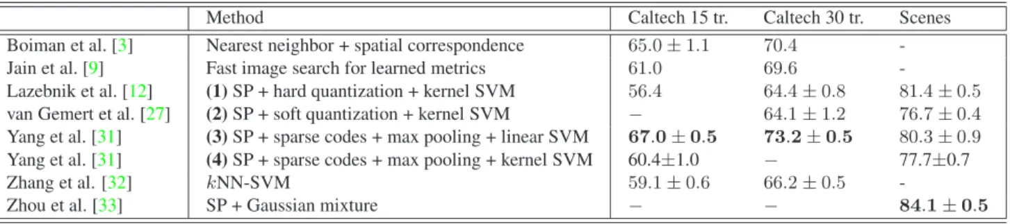
Method Caltech 15 tr. Caltech 30 tr. Scenes Boiman et al. [3] Nearest neighbor + spatial correspondence 65.0±1.1 70.4

-Jain et al. [9] Fast image search for learned metrics 61.0 69.6

-Lazebnik et al. [12] (1)SP + hard quantization + kernel SVM 56.4 64.4±0.8 81.4±0.5

van Gemert et al. [27] (2)SP + soft quantization + kernel SVM − 64.1±1.2 76.7±0.4

Yang et al. [31] (3)SP + sparse codes + max pooling + linear SVM 67.0±0.5 73.2±0.5 80.3±0.9

Yang et al. [31] (4)SP + sparse codes + max pooling + kernel SVM 60.4±_1.0 − _77.7±_0.7

Zhang et al. [32] k_NN-SVM 59.1±0.6 66.2±0.5

-Zhou et al. [33] SP + Gaussian mixture − − 84.1±0.5

Table 2. Results obtained by several recognition schemes using a single type of descriptors. Bold numbers in parentheses preceding the method description indicate methods reimplemented in this paper. SP: spatial pyramid.

Caltech-101 [6] and Scenes datasets [12] as benchmarks. These datasets respectively comprise 101 object categories (plus a ”background” category) and fifteen scene categories. Following the usual procedure [12, 31], we use 30 train-ing images and the rest for testtrain-ing (with a maximum of 50 test images) on the Caltech-101 dataset, and 100 training images and the rest for testing on the Scenes dataset. Ex-periments are conducted over 10 random splits of the data, and we report the mean accuracy and its standard devia-tion. Hyperparameters of the model are selected by cross-validation within the training set. The general architecture follows [12]. Low-level descriptorsx_{iare 128-dimensional}

SIFT descriptors [18] of16×16patches. The descriptors are extracted on a dense grid rather than at interest points, as this procedure has been shown to yield superior scene classification [17]. Pooling regionsmcomprise the cells of

4_×4,2_×2and1_×1grids (forming a three-level pyramid). We use the SPAMS toolbox [1] to compute sparse codes.

3.1. Interaction Between Modules

Here, we perform a systematic cross evaluation of all the coding, pooling and classifier types presented in Sec.2, with SIFT descriptors extracted densely every 8 pixels. Results are presented on Table1. The ranking of performance when changing a particular module (e.g., coding) is quite consis-tent:

• Sparse coding improves over soft quantization, which improves over hard quantization;

• Max pooling almost always improves over average pooling, dramatically so when using a linear SVM; • The intersection kernel SVM performs similarly or

better than the linear SVM.

In particular, the global feature obtained when using hard vector quantization with max pooling achieves high

accu-racy with a linear classifier, while beingbinary, and merely recording the presence or absence of each codeword in the pools. While much research has been devoted to devising the best possible coding module, our results show that with linear classification, switching from average to max pooling increases accuracy more than switching from hard quanti-zation to sparse coding. These results could serve as guide-lines for the design of future architectures.

For comparison, previously published results obtained using one type of descriptors on the same dataset are shown on Table 2. Note that better performance has been re-ported with multiple descriptor types (e.g., methods using multiple kernel learning have achieved 77.7%_±0.3 [7] and 78.0%±0.3 [2, 28] on Caltech-101 with 30 train-ing examples), or subcategory learntrain-ing (83%on Caltech-101 [26]). The coding and pooling module combinations used in [27,31] are included in our comparative evaluation (bold numbers in parentheses on Tables 1 and2). Over-all, our results confirm the experimental findings in these works, except that we do not find superior performance for the linear SVM, compared to the intersection kernel SVM, with sparse codes and max pooling, contrary to Yang et al. [31]. Results of our reimplementation are similar to those in [12]. The better performance than that reported by Van Gemert et al. [27] or Yang et al. [31] on the Scenes is not surprising since their baseline accuracy for the method in [12] is also lower, which they attributed to implementa-tion differences. Discrepancies with results from Yang et al. [31] may arise from their using a differentiable quadratic hinge loss instead of the standard hinge loss in the SVM, and a different type of normalization for SIFT descriptors.

3.2. Macrofeatures and denser SIFT sampling

In convolutional neural networks (e.g., [16, 23]), spa-tial neighborhoods of low-level features are encoded jointly. On the other hand, codewords in bag-of-features methods usually encode low-level features at a single location (see Fig.1). We propose to adapt the joint encoding scheme to the spatial pyramid framework.

Jointly encodingLdescriptors in a local spatial neigh-borhood_Liamounts to replacing Eq. (1) by:

α_i=f([xT

i1· · ·x

T iL]

T_{), i}

1,· · · , iL∈ Li. (9)

In the following, we call macrofeatures vectors that jointly encode a small neighborhood of SIFT descriptors. The encoded neighborhoods are squares determined by two parameters: the side of the square (e.g., 2 × 2 square on Fig.1), and a subsampling parameter determining how many SIFT descriptors to skip along each dimension when selecting neighboring features. For example, a3_×3 macro-feature with a subsampling parameter of 2 jointly encodes 9 descriptors out of a6_×6grid, skipping every other column and row.

Figure 1. Standard features encode the SIFT features at a single spatial point. Macrofeatures jointly encode small spatial neigh-borhoods of SIFT features (i.e., the input of the coding module is formed by concatenating nearby SIFT descriptors).

We have experimented with different macrofeature pa-rameters, and denser sampling of the underlying SIFT de-scriptor map (e.g., extracting SIFT every 4 pixels instead of 8 pixels as in the baseline of [12]). We have tested sampling densities of 2 to 10, and macrofeatures of side length 2 to 4 and subsampling parameter 1 to 4. When using sparse cod-ing and max poolcod-ing, the best parameters (selected by cross-validation within the training set) for SIFT sampling den-sity, macrofeature side length and subsampling parameter are respectively of 4, 2, 4 for the Caltech-101 dataset, and 8, 2, 1 for the Scenes dataset. Our results (Table1, bottom) show that large improvements can be gained on the Caltech-101 benchmark, by merely sampling SIFT descriptors more finely, and jointly representing nearby descriptors, yielding a classification accuracy of 75.7%, which to the best of our knowledge is significantly better than all published classifi-cation schemes using a single type of low-level descriptor. However, we have not found finer sampling and joint encod-ing to help recognition significantly on the Scenes dataset.

4. Discriminative dictionaries

The feature extraction schemes presented so far are all unsupervised. When using sparse coding, an adaptive dic-tionary is learned by minimizing a regularized reconstruc-tion error. While this ensures that the parameters of the dic-tionary are adapted to the statistics of the data, the dictio-nary is not optimized for the classification task. In this sec-tion, we introduce a novel supervised method to learn the dictionary.

Several authors have proposed methods to obtain dis-criminative codebooks. Lazebnik and Raginsky [11]

incor-porate discriminative information by minimizing the loss of mutual information between features and labels during the quantization step. Winn et al. [30] prune a large codebook iteratively by fusing codewords that do not contribute to dis-crimination. However these methods are optimized for vec-tor quantization. Mairal et al. [20] have proposed an algo-rithm to train discriminative dictionaries for sparse coding, but it requires each encoded vector to be labelled. Instead, the approach we propose is adapted to global image statis-tics.

With the same notation as before, let us consider the ex-traction of a global image representation by sparse coding and average pooling over the whole imageI:

ˆ

xT

i = [xTi1· · ·x

T

iL], i1,· · · , iL∈ Li, (10)

α_{i= argmin}

α

L(α_,D₎,_kxˆ_i−Dα_k2

2+λkαk1, (11) h₌ 1

|I_| X

i∈I

αi, (12)

z ₌h_{. (13)}

Consider a binary classification problem. Letz(n)

de-note the global image representation for the n-th training image, andyn ∈ {−1,1}the image label. A linear

classi-fier is trained by minimizing with respect to parameterθthe regularized logistic cost:

Cs=

1

N N

X

n=1

log1 +e−ynθTz(n)_+λ

rkθk22, (14)

whereλrdenotes a regularization parameter. We use

logis-tic regression because its level of performance is typically similar to that of linear SVMs but unlike SVMs, its loss function is differentiable. We want to minimize the super-vised costCswith respect toDto obtain a more

discrimi-native dictionary. Using the chain rule, we obtain: ∂Cs

∂D_jk =−

1

N N

X

n=1

yn

1₋σ(ynθ.z(n))

θT∂z(n) ∂D_jk (15) ∂z(n)

∂D_jk =

1 |I(n)_|

X

i∈I(n)

∂α(n)

i

∂D_jk, (16)

where σ denotes the sigmoid function σ(x) = 1/(1 + exp(−x)). We need to compute the gradient ∇D(αi). Since the αi minimize Eq. (11), they

verify:

α_{= (}DαTDα)−1(DαTxˆ−λsign(α)), (17) where we have dropped subscriptito limit notation clutter, andDα denotes the columns corresponding to the active set ofα_{(i.e., the few columns of}D_{used in the} decomposi-tion of the input). Note that this formula cannot be used to

computeα_{, as parts of the right-hand side of the equation}

depend onα_{itself, but it can be used to compute a gradient}

onceα_{is known. When perturbations of the dictionary are}

small, the active set ofα_{often stays the same (since the}

cor-relation between the atoms of the dictionary and the input vector varies continuously with the dictionary). Assuming that it is constant, we can compute the gradient of the active coefficients with respect to the active columns ofD_(setting it to0elsewhere):

∂α˜_k ∂(Dα)_ij

=b_iA_{kj −}α˜_jC_{ki, (18)} A_,(DαTDα)−1, (19) b_,x_ˆ−Dα_{, (20)}

C,ADαT, (21) whereα˜_{kdenotes thek-th non-zero component of}α_.

We train the discriminative dictionary by stochastic gra-dient descent [4,14]. Recomputing the sparse decompo-sitions α_{i at each location of a training image at each}

it-eration is costly. To speed-up the computation while re-maining closer to global image statistics than with individ-ual patches, we approximatez(n)_{by pooling over a random}

sample of ten locations of the image. Furthermore, we up-date only a random subset of coordinates at each iteration, since computation of the gradient is costly. We then test the dictionary with max pooling and a three-layer spatial pyra-mid, using either a linear or intersection kernel SVM.

Unsup Discr Unsup Discr Linear 83.6±0.4 84.9±0.3 84.2±0.3 85.6±0.2

Intersect 84.3±0.5 84.7±0.4 84.6±0.4 85.1±0.5

Table 3. Results of learning discriminative dictionaries on the Scenes dataset, for dictionaries of size 1024 (left) and 2048 (right), with 2×2 macrofeatures and grid resolution of 8 pixels,

We compare performance of dictionaries of sizes 1024 and 2048 on the Scenes dataset, encoding 2_×2 neighbor-hoods of SIFT. Results (Table3) show that discriminative dictionaries perform significantly better than unsupervised dictionaries. A discriminative dictionary of 2048 code-words achieves 85.6% correct recognition performance, which to the best of our knowledge is the highest pub-lished classification accuracy on that dataset for a single fea-ture type. Discriminative training of dictionaries with our method on the Caltech-101 dataset has yielded only very little improvement, probably due to the scarcity of training data.

5. Comparing Average and Max Pooling

av-erage pooling generalizes to many combinations of cod-ing schemes and classifiers. Several authors have already stressed the efficiency of max pooling [10, 31], but they have not given theoretical explanations to their findings. In this section, we study max pooling in more details theoreti-cally and experimentally.

5.1. A Theoretical Comparison of Pooling Strategies

With the same notation as before, consider a binary lin-ear classification task over cluttered images. Pooling is per-formed over the whole image, so that the pooled feature

h_{is the global image representation. Linear classification}

requires distributions ofh_{over examples from positive and}

negative classes (henceforth denoted by+and₋) to be well separated.

We model the distribution of image patches of a given class as a mixture of two distributions [21]: patches are taken from the actual class distribution (foreground) with probability(1−w), and from a clutter distribution (back-ground) with probability w, with clutter patches being present in both classes (+or₋). Crucially, we model the amount of clutterwas varying between images (while being fixed for a given image).

There are then two sources of variance for the distribu-tionp(h_{): the intrinsic variance caused by sampling from a}

finite pool for each image (which causes the actual value of

h_{over foreground patches to deviate from its expectation),}

and the variance ofw(which causes the expectation of h

itself to fluctuate from image to image depending on their clutter level). If the pool cardinality N is large, average pooling is robust to intrinsic foreground variability, since the variance of the average decreases in _N1.This is usually not the case with max pooling, where the variance can in-crease with pool cardinality depending on the foreground distribution.

However, if the amount of clutterwhas a high variance, it causes the distribution of the average over the image to spread, as the expectation ofh_{for each image depends on}

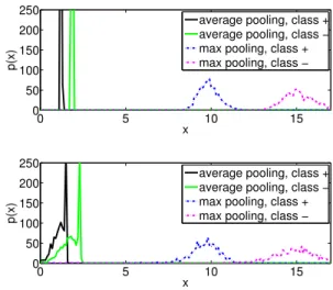
w. Even if the foreground distributions are well separated, variance in the amount of clutter creates overlap between the mixture distributions if the mean of the background dis-tribution is much lower than that of the foreground distri-butions. Conversely, max pooling can be robust to clutter if the mean of the background distribution is sufficiently low. This is illustrated on Fig.2, where we have plotted the empirical distributions of the average of 10 pooled features sharing the same parameters. Simulations are run using 1000 images of each class, composed ofN = 500patches. For each image, the clutter levelwis drawn from a truncated normal distribution with either low (top) or high (bottom) variance. Local feature values at each patch are drawn from a mixture of exponential distributions, with a lower mean for background patches than foreground patches of either

0 5 10 15

0 50 100 150 200 250

x

p(x)

average pooling, class + average pooling, class − max pooling, class + max pooling, class −

0 5 10 15

0 50 100 150 200 250

x

p(x)

average pooling, class + average pooling, class − max pooling, class + max pooling, class −

Figure 2. Empirical probability densities of x = 1

K

PK

j=1hj,

simulated for two classes classes of images forming pools of car-dinalityN= 500. The local features are drawn from one of three exponential distributions. When the clutter is homogeneous across images (top), the distributions are well separated for average pool-ing and max poolpool-ing. When the clutter level has higher variance (bottom), the max pooling distributions (dashed lines) are still well separated while the average pooling distributions (solid lines) start overlapping.

class. When the clutter has high variance (Fig.2, bottom), distributions remain well separated with max pooling, but have significant overlap with average pooling.

We now refine our analysis in two cases: sparse codes and vector quantized codes.

5.1.1 Sparse Codes.

In the case of a positive decomposition over a dictionary, we model the distribution of the value of featurejfor each patch by an exponential distribution with meanµj, variance µ2

j, and densityf(x) = _{µ j}1 exp

−x

µj_{. The choice of an} expo-nential distribution (or a Laplace distribution when decom-positions are not constrained to be positive) to model sparse codes seems appropriate because it is highly kurtotic and sparse codes have heavy tails.

The corresponding cumulative distribution function is F(x) = 1₋e−µjx _{. The cumulative distribution function of} the max-pooled feature isFN_{(x) = (1−e}−µjx₎N _{for a pool}

of sizeN. Clutter patches are sampled from a distribution of meanµb.LetNf andNb denote respectively the

num-ber of foreground and background patches,N =Nf+Nb.

AssumingNf andNb are large, Taylor expansions of the

cumulative distribution functions of the maxima yield that 95% of the probability mass of the maximum over the back-ground patches will be below 95% of the probability mass of the maximum over the foreground patches provided that

Nb < |log(0.95)|

_N

f |log(0.05)|

µj_µb

. In a binary discrimi-nation task between two comparatively similar classes, if an image is cluttered by many background patches, with µb ≪ µ+j andµb ≪ µ−j, max-pooling can be relatively

immune to background patches, while average-pooling can create overlap between the distributions (see Fig.2). For example, ifµb < 2µj andNf = 500, having fewer than Nb < 1400background patches virtually guarantees that

the clutter will have no influence on the value of the maxi-mum. Conversely, ifNb<N59f ≤

|log(0.95)|

|log(0.05)|Nf, clutter will

have little influence for µb up to µj. Thus, max-pooling

creates immunity to two different types of clutter: ubiqui-tous with low feature activation, and infrequent with higher activation.

However, a downside is that the ratio of the mean to the standard deviation of the maximum distribution does not decrease as √1

N, as in the case of the distribution of the

average. In fact, the mean and variance of the maximum distribution overN samples can be shown to be:

ν= (_H(N)).µj, σ2=

N

X

l=1 1

l(2H(l)− H(N)) !

.µ2_j, where_H(k) =Pk

i=1 1

i denotes the harmonic series, which

grows likelog(k).It can be shown that:

N

X

l=1 1

l(2H(l)− H(N)) = log(N) +O(1), so that the ratio ν_σ decreases like √ 1

log(N). Thus, if the

pool cardinality is too small, the distributions of foreground patches from both classes will be better separated with av-erage pooling than max pooling.

5.1.2 Vector Quantization.

We model binary patch codes for feature j by i.i.d. Bernoulli random variables of mean µj. The

distribu-tion of the average-pooled feature also has mean µj,

and its variance decreases like _N1. The maximum is a Bernoulli variable of mean 1₋(1₋µj)N and variance

(1₋(1₋µj)N)(1−µj)N.Thus, it is 1 with probability

0.95 ifN ≥ log(1log(0−.05)µj)≈

|log(0.05)|

µj ,and 0 with probability 0.95 ifN ≤ log(1log(0−.95)µj) ≈

|log(0.95)|

µj ,forµj ≪1. The sep-arability of classes depends on sample cardinalityN.There exists a sample cardinalityN for which the maximum over class+is 0 with probability 0.95, while the maximum over class₋is 1 with probability 0.95, if:

µ−_j µ+_j >

log(0.05) log(0.95), e.g. if

µ−_j µ+_j >59.

AsP

jµj = 1in the context of vector quantization,µj

be-comes very small on average if the codebook is very large. Forµj ≪1, the characteristic scale of the transition from 0

to 1 is _µ1

j, hence the pooling cardinality range correspond-ing to easily separable distributions can be quite large if the mean over foreground patches from one class is much higher than both the mean over foreground patches from the other class and the mean over background patches.

5.2. Experimental Validation

Our analysis suggests that there may be a purely statis-tical component to the improvement seen with max pool-ing when uspool-ing pyramids instead of plain bags of features. Taking the maximum over several pools of smaller cardinal-ity may lead to a richer estimate, since max pooling differs from average pooling in two important ways:

• the maximum over a pool of smaller cardinality is not merely an estimator of the maximum over a larger pool;

• the variance of the maximum is not inversely propor-tional to pool cardinality, so that summing over sev-eral estimates (one for each smaller pool) can provide a smoother output than if pooling had merely been per-formed over the merged smaller pools.

We have tested this hypothesis by comparing three types of pooling procedures: standard whole-image and two-level pyramid pooling, and random two-level pyramid pooling, where local features are randomly permuted before being pooled, effectively removing all spatial information.

For this experiment, SIFT features are extracted densely every 8 pixels, and encoded by hard quantization over a codebook of size 256 for Caltech-101, 1024 for the Scenes. The pooled features are concatenated and classified with a linear SVM, trained on 30 and 100 examples for Caltech-101 and the Scenes, respectively.

Caltech 101 15 Scenes Pyramid 1×1 2×2 1×1 2×2

Avg, random 31.7±1.0 29.5±0.5 71.0±0.8 69.4±0.8

Avg, spatial 43.2±1.4 73.2±0.7

Max, random 26.2±0.7 33.1±0.9 69.5±0.6 72.8±0.3

Max, spatial 50.7±0.8 77.2±0.6

Table 4. Classification accuracy for different sets of pools and pooling operators.

Results (Table4) show that with max pooling, a substan-tial part of the increase in accuracy seen when using a two-level pyramid instead of a plain bag of features is indeed still present when locations are randomly shuffled. On the contrary, the performance of average pooling tends to dete-riorate with the pyramid, since the added smaller, random pools only contribute noisier, redundant information.

6. Discussion

By deconstructing the mid-level coding step of a well-accepted recognition architecture, it appears that any pa-rameter in the architecture can contribute to recognition per-formance; in particular, surprisingly large performance in-creases can be obtained by merely sampling the low-level descriptor map more finely, and representing neighboring descriptors jointly. We have presented a scheme to train su-pervised discriminative dictionaries for sparse coding; our ongoing research focuses on extending this framework to the much harder PASCAL datasets, on which methods very similar to the ones discussed in this paper [31] currently define the state of the art. We plan to combine our discrimi-native sparse training algorithm with the various techniques (e.g., local coordinate coding) that have been successful on PASCAL. Another research direction we are pursuing is the analysis of pooling schemes. Understanding pooling opera-tors is crucial to good model design, since common heuris-tics suited to average pooling may be suboptimal in other contexts. In this paper, we have only briefly touched upon the statistical properties of max pooling. We are currently investigating how to expand these theoretical insights, and turn them into guidelines for better architecture design. Acknowledgements. This work was funded in part by NSF grant EFRI/COPN-0835878 to NYU, and ONR con-tract N00014-09-1-0473 to NYU. We would like to thank Sylvain Arlot, Olivier Duchenne and Julien Mairal for help-ful discussions.

References

[1] http://www.di.ens.fr/willow/SPAMS/.3

[2] http://www.robots.ox.ac.uk/˜vgg/software/MKL/.4

[3] O. Boiman, I. Rehovot, E. Shechtman, and M. Irani. In De-fense of Nearest-Neighbor Based Image Classification. In

CVPR, 2008. 3

[4] L. Bottou. Online algorithms and stochastic approximations. In D. Saad, editor,Online Learning and Neural Networks. Cambridge University Press, Cambridge, UK, 1998. 5

[5] N. Dalal and B. Triggs. Histograms of oriented gradients for human detection. InCVPR, 2005. 1

[6] L. Fei-Fei, R. Fergus, and P. Perona. Learning generative vi-sual models from few training examples. InCVPR Workshop GMBV, 2004.3

[7] P. Gehler and S. Nowozin. On Feature Combination for Mul-ticlass Object Classification. InICCV, 2009.4

[8] G. Hinton and R. R. Salakhutdinov. Reducing the dimen-sionality of data with neural networks. Science, 313(5786), 2006.1

[9] P. Jain, B. Kulis, and K. Grauman. Fast image search for learned metrics. InCVPR, 2008. 3

[10] K. Jarrett, K. Kavukcuoglu, M. Ranzato, and Y. LeCun. What is the best multi-stage architecture for object recog-nition? InICCV, 2009.6

[11] S. Lazebnik and M. Raginsky. Supervised Learning of Quan-tizer Codebooks by Information Loss Minimization. PAMI, 21, 2008.4

[12] S. Lazebnik, C. Schmid, and J. Ponce. Beyond bags of features: Spatial pyramid matching for recognizing natural scene categories. InCVPR, 2006. 1,2,3,4

[13] Y. LeCun, L. Bottou, Y. Bengio, and P. Haffner. Gradient-based learning applied to document recognition. Proceed-ings of the IEEE, 86(11):2278–2324, November 1998.1

[14] Y. LeCun, L. Bottou, G. Orr, and K. Muller. Efficient back-prop. In G. Orr and M. K., editors,Neural Networks: Tricks of the trade. Springer, 1998.5

[15] H. Lee, A. Battle, R. Raina, and A. Y. Ng. Efficient sparse coding algorithms. InNIPS, 2006.2

[16] H. Lee, R. Grosse, R. Ranganath, and A. Ng. Convolutional deep belief networks for scalable unsupervised learning of hierarchical representations. InICML, 2009.1,4

[17] F.-F. Li and P. Perona. A bayesian hierarchical model for learning natural scene categories. InCVPR, 2005.3

[18] D. Lowe. Distinctive image features from scale-invariant keypoints.Int. J. of Comp. Vision, 60(4):91–110, 2004.1,3

[19] J. Mairal, F. Bach, J. Ponce, and G. Sapiro. Online Dictio-nary Learning for Sparse Coding. InICML, 2009.2

[20] J. Mairal, F. Bach, J. Ponce, G. Sapiro, and A. Zisserman. Supervised Dictionary Learning. InNIPS, 2009.5

[21] T. Minka. Expectation Propagation for approximate Bayesian inference. InUAI, 2001.6

[22] B. A. Olshausen and D. J. Field. Sparse coding with an over-complete basis set: a strategy employed by V1? Vision Re-search, 37:3311–3325, 1997. 2

[23] M. Ranzato, Y. Boureau, and Y. LeCun. Sparse feature learn-ing for deep belief networks. InNIPS 2007, 2007.1,4

[24] T. Serre, L. Wolf, and T. Poggio. Object recognition with features inspired by visual cortex. InCVPR, 2005. 1

[25] J. Sivic and A. Zisserman. Video Google: A text retrieval approach to object matching in videos. InICCV, 2003.1,2

[26] S. Todorovic and N. Ahuja. Learning subcategory relevances for category recognition. InCVPR, 2008.4

[27] J. C. van Gemert, C. J. Veenman, A. W. M. Smeulders, and J. M. Geusebroek. Visual word ambiguity.PAMI, (in press), 2010.2,3,4

[28] A. Vedaldi, V. Gulshan, M. Varma, and A. Zisserman. Mul-tiple kernels for object detection. InProc. Int. Conf. Comp. Vision, 2009.4

[29] S. Winder and M. Brown. Learning local image descriptors. InCVPR, 2007.1

[30] J. Winn, A. Criminisi, and T. Minka. Object categorization by learned universal visual dictionary. InICCV 2005.5

[31] J. Yang, K. Yu, Y. Gong, and T. Huang. Linear Spatial Pyra-mid Matching Using Sparse Coding for Image Classification. InCVPR, 2009.1,2,3,4,6,8

[32] H. Zhang, A. C. Berg, M. Maire, and J. Malik. SVM-KNN: Discriminative nearest neighbor classification for visual cat-egory recognition. InCVPR, 2006.3

[33] X. Zhou, X. D. Zhuang, H. Tang, M. H. Johnson, and T. S. Huang. A novel gaussianized vector representation for natu-ral scene categorization. InICPR, 2008.3