Filter Models of CDM Measurement Channels and TLP
Device Transients
Timothy J. Maloney
1and Abishai Daniel
21Intel Corporation, 2200 Mission College Blvd., SC9-09, Santa Clara, CA 95054 USA tel.: 408-765-9389 e-mail: [email protected]
2Intel Corporation, RA1-329, Hillsboro, OR
This paper is co-copyrighted by Intel Corporation and the ESD Association
Abstract – Charged Device Model (CDM) waveforms are fast enough to be altered considerably by the oscilloscope used. Step response of CDM measurement channels allow time-domain finite impulse response (FIR) filters to be formulated in software. Similar analytic methods allow filter-like representation of devices as measured by transmission-line pulsing (TLP).
I. Introduction
Our understanding of the charged device model of ESD has, over the past quarter-century, been enhanced by advances in measurement technology. Ever-faster oscilloscopes have helped us distinguish between the properties of the CDM pulse itself and the associated measurement channel. Digital storage scopes have progressed past 1 GHz bandwidth to 3, 6, 8 and even 12 GHz models being accessible to many workers, so there are now fewer surprises in the CDM waveform. But slower scopes (i.e., down to 1 GHz nominal) are still in common use and should be evaluated for their continued service to industry CDM standards. Important recent work [1] shows differences among several scopes in the frequency domain, and compares Ipeak and CDM pulse properties among the scopes. This work will focus on a fast and efficient time-domain method of scope characterization (step response), and will derive filter properties sufficient to predict time and frequency behavior of the measurement channel. This is possible because the step response does not throw away phase information, and keeps enough amplitude information to allow at least a few filter poles to be calculated. The non-ideal fast step generator is a limitation, of course, but, using a fast oscilloscope, the step itself can be modeled as a filter, and then the slower scopes are readily characterized by noting differences. At this point, there is enough information to extract a (software) finite impulse response (FIR) filter model of the scope channel of interest, and use it to predict measured waveforms of any kind.
The filter theory for step response of the measurement channel as above is derived from a very general theory of linear, time-invariant (LTI) networks [2]. It turns out that the same sort of analysis can be applied
to the transmission line pulsing (TLP) problem of characterizing a device’s TLP transient behavior in some concise, easily recordable way. Devices do not always cooperate by being linear in all respects, as we well know from decades of looking at steady-state response, but the filter method to be discussed here can still be applied because any function can be linearized at a particular operating point. Accordingly, a power series in complex frequency (s=+j) for generalized impedance or admittance, Z(s)=1/Y(s)=R1(1+x1s+x2s2+…), can be readily derived by considering the device to be a kind of filter.
II. CDM Measurement Channels
1. Filters and Moment Extraction
The simplest approach to characterizing an unknown network is to assume that it is, at least within some range, an LTI network. Knowing the impulse response of such a network should be sufficient to predict its behavior under all conditions, subject to the constraints imposed. Elementary network theory tells us that a step response is the integral of impulse response, and therefore that the response to a step generator is sufficient to find the impulse response, and network transfer function, of the circuit in question.
...) 1
( )
( 3
3 2 2 1
0
a s a s a s s
V s
V , (1)
where the complex frequency coefficients an capture the finite rise time and other features of the waveform. To find the series an, we appeal to the method of [3], and more completely described in [4], of successive integration of the waveform, also called moment extraction. Let us assume the step generator has a nominal output impedance of Z0 (e.g., 50 ohms) and we measure the response at a well-designed load Z0. The step height V0 (a measured V0 means the step source height is 2V0) thereby gives the 0th order coefficient. The transform of the time-dependent function V(t)-V0 is then the function V(s)-V0/s=V0a1+V0a2s+…, which can be normalized (divided by V0) and integrated (divided by s) to give a new step height a1 (a1 is expected to be negative, as the generator is an imperfect step). This process is repeated to give a2, a3, and as many coefficients as desired, or as noise limits allow.
An even more descriptive network function for V(s) (or to be exact, the normalized impulse response sV(s)/V0) would be a ratio of polynomials, well- known in circuit theory as the pole-zero description (as the polynomials can be factored). This general function also applies to amplifier response as in an oscilloscope and would be, as described in [3-5], a network impulse response function like
,
1
1
)
(
22 1
2 2 1
m m
n n
s
b
s
b
s
b
s
a
s
a
s
a
s
H
(2) where m>n. As Elmore [5] stated in 1948, citing even earlier references on LTI networks, H(s) can be “the normalized system function…of a stable amplifier containing a finite number of lumped circuit elements…where the coefficients ai and bi are real, m>n, and the poles…all lie in the left half of the complex s-plane.” This is a good way to describe well-designed step generators and oscilloscope amplifiers, then and now. In Eq. 2, it is convenient to expand the functions in powers of s and compute coefficients an as above, as we expect the impulse response to decay away as t. Such an expansion of (2) appears in signal integrity literature [6] and elsewhere [4],
2 2 1 1 1 2 2 1
1
)
(
)
(
1
)
(
s
a
b
s
a
b
b
a
b
s
H
3 31 2 1 1 1 2 2 1 2 1 3
3
2
)
(
a
b
a
b
b
b
a
b
a
b
b
s
(3)
This will prove to be one of several powerful tools in extracting our best estimate of an impulse response.
Note that if we are measuring a presumed 2-pole step generator of unit magnitude
)
1
(
1
)
(
22 1
s
b
s
b
s
s
V
, (4)Eq. (3) tells us the moment extraction as described above and in [3,4] will give us measured voltage
s
s
b
b
s
b
s
V
m(
)
1
1
(
12
2)
2
. (5)We then expect this signal as filtered by another transfer function, one for the oscilloscope, to produce an expression for the final measured waveform. Using Eqs. (3)-(5), it should be possible to extract oscilloscope parameters readily, particularly if we know we are starting with a very fast step compared to the response of the target scope.
2. Importance of 10-90% Rise Time
A useful oscilloscope study [7] began with the Gaussian filter model of scope response, yet also showed that a two-pole pseudo-Gaussian gives a very similar result, and solved the problem of where to locate t=0. It is useful at this point to recall [8] that the poles of a 2-pole network are
) 1
( 2
0 2 ,
1 D D
p
, (6)where D is the damping factor and 0 is a characteristic frequency. Note that complex conjugate poles result for D<1, and this is expected when our step response produces ringing.
In [7] (which we will call M-S), the pseudo-Gaussian was also shown to follow the Gaussian convolution pattern of quadrature addition of rise times, if they are 10-90% rise times. This means that if a step function with 10-90% rise time 1 is observed on a scope with intrinsic 10-90% rise time 2, the observed 10-90% rise time will be
2 2 2
1
r
. (7)dB
f
32
3396
.
0
. (8)Mittemayer and Steininger [7] also show that
4 2 2
0
3 1 2 2 1 2 2
2 D D D
f dB
(9)
which, for their favorite case of D=0.707 (1/2), reduces to 0/2. This choice for D also maximizes the Elmore Delay [5] e=2D/0 in our intended range of 0.6<D<1, meaning that the 10-90% rise time is minimized, given circuit elements that determine f3dB and e. The 2-pole filter network has a transfer function
2 2 1
1
1
)
(
s
b
s
b
s
X
; b1= e and b2=1/02, or2
0 0
2 1
1 )
(
j D
j
X . (10)
We want to formulate 2-pole models for the step source and the oscilloscopes so that we can calculate what happens to fast waveforms, first the steps and then the CDM waveforms. Note that we now have two ways of finding the filter parameters b1 and b2, we can extract moments as above and as in [3,4], or we can follow M-S and use the 10-90% rise time. With M-S, once we use Eq. (7) to adjust for the finite rise time of the step source, we have a unique value of f3dB from Eq. (8) that is justified as long as we see some slight amount of overshoot in the measured step. It then remains to choose acceptable values of D and 0 in accordance with Eq. (9), where 0.6<D<1. For the oscilloscope we focus on D=0.707, as for M-S it “suits favorably to our observations and those reported in the literature.” We will then cross-check our choice with the Elmore Delay (b1) and the next parameter (b2) as measured by moment extraction, described earlier and in [3,4].
We expect parameters b1, b2 for each oscilloscope to be sufficient filter parameters. Thus, an impulse response in the time domain can be computed through the inverse Laplace Transform, and the filtering effect on any waveform can be computed through convolution [9].
The present study uses a fast step source and an 8GHz scope as a baseline for characterization of two nominal 1 GHz scopes. As a result, the filter functions of the two slow scopes represent mappings from the fast scope, i.e., a measure of how much worse a slow scope is compared to the fast one. Were
for example, the parameter b1 for the 1GHz scope might be under 100 psec instead of over 200 psec— the 1GHz instrument is the same, but understandably has less effect on a waveform baselined to 2 GHz as compared to 8 GHz. It will become clear that as we raise the fidelity of our baseline equipment, we get closer to an “unfiltered” source as far as the target scope is concerned.
3. Step Source and Channel Models
We start with the step source (Tektronix 067-1338-00) as measured on the Tektronix 8GHz (DPO70804) oscilloscope. From Eq. (8), a 10-90% rise time of 57.8 psec gives an f3dB of 5.875 GHz; then matching the general features of the overshoot (Section II.1) yields D=0.62, 0=32.9 GHz and therefore
e=2D/0=37.7 psec. The result is shown in Figure 1.
Figure 1. Fast step (57.8 psec, 10-90%) for 8 GHz channel and 2-pole approximation at left.
The 2-pole model of the step source has the expected discontinuous derivative at the origin and matches the scope waveform in the 10-90% rise time aspect best. The Elmore Delay e as extracted from the scope waveform is sensitive to the choice of t=0 and matches the 2-pole value of about 38 psec if one compensates for the continuous derivative at the origin for the actual scope signal. However, the next integral (finding a2=b12-b2) of the scope waveform yields a b2 value too small to give overshoot. Thus we prefer the 10-90% 2-pole model for now. The voltage source model for unit magnitude expressed as in Eq. (4), adding a pole at zero to make it a step, is
)
924
7
.
37
1
(
1
)
(
2s
s
s
s
V
, (11)where s is in THz and coefficients are in psec and (psec)2.
Fast step on 8 GHz scope
0 0.2 0.4 0.6 0.8 1 1.2
0 100 200 300 400
time, psec
N
o
rm
al
iz
ed
u
n
it
s
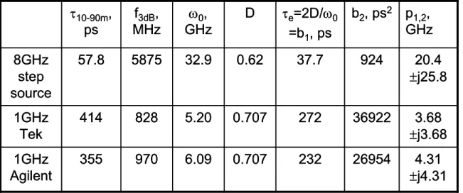
Table I. Measured and derived parameters for the step source and two 1 GHz oscilloscopes, using the 10-90% method. Note that b1, b2,
and p1,2 are derived from 0 and D.
With an apparent f3dB of 5.875 GHz, the step source appears to be about evenly split at about 40 psec each for (1) actual step generator rise time, and (2) intrinsic scope rise time, if scope f3dB8 GHz and assuming Eq. (7) applies. This is as expected and should provide a good baseline for the 1 GHz scope measurements.
The parameters for the 1 GHz Tektronix (TDS684B) and Agilent (DSO7104A) scopes were taken from measured 10-90% rise times (=10-90m) in similar fashion after correcting for the finite step rise time as in Eq. (7). However, the step was known to be so fast that the adjustment was only 3-5 picoseconds among several hundred, so the mapping from 8 GHz data is very close to a response to an unfiltered signal.
Table I contains the deduced 2-pole filter model parameters for the step source and the oscilloscopes, based on the measured 10-90% step response in the first column.
Figure 2 shows the application of the 2-pole step source model to the 1GHz Tek scope model to form a 4-pole step. This is compared to the measured step response on the 1 GHz Tektronix scope, showing the expected match to 10-90% rise time and other general features. The 4-pole model transfer function is
.
)
37125
272
1
)(
924
7
.
37
1
(
1
)
(
2 21 8
s
s
s
s
s
X
T
(12)
and the step is formed by integration, i.e., dividing by s. Conversion to time domain is done by Heaviside inversion [10].
Figure 2. 4-pole model of a fast step filtered by the 1 GHz Tek scope (left), compared with the measured response to a fast step (right), delayed for clarity.
The measured 1 GHz scope waveforms were also integrated to give values of b1 and b2 by the moment method as described in Section II.1. Again, b1 would fit after compensating for the initial concave-upward character of the step. For the Tek scope, the measured b2 suggested a D=0.83, not far off from our ultimate choice based on the 10-90% method, but a little less representative of the overshoot as captured in Fig. 2. As the 10-90% method is really easiest to implement, we proceed to seeing how well it predicts measured CDM waveforms.
III.
Convolution FIR Filtering of
CDM Waveforms
Using the 2-pole models of the CDM measurement channel, we are now equipped to take CDM waveforms from a high frequency oscilloscope and predict the waveform to be seen on a
lower-Fast step on 1 GHz Tek scope
0 0.2 0.4 0.6 0.8 1 1.2
0 200 400 600 800 1000 1200 1400
time, psec
N
o
rm
al
iz
ed
vo
lt
ag
e
4-pole model 1 GHz scope data
model
Fast step on 1 GHz Tek scope
0 0.2 0.4 0.6 0.8 1 1.2
0 200 400 600 800 1000 1200 1400
time, psec
N
o
rm
al
iz
ed
vo
lt
ag
e
4-pole model 1 GHz scope data
model
4.31
j4.31
26954
232
0.707
6.09
970
355
1GHz
Agilent
3.68
j3.68
36922
272
0.707
5.20
828
414
1GHz
Tek
20.4
j25.8
924
37.7
0.62
32.9
5875
57.8
8GHz
step
source
p
1,2,
GHz
b
2, ps
2
e=2D/
0=b
1, ps
D
0,
GHz
f
3dB,
MHz
10-90m,
ps
4.31
j4.31
26954
232
0.707
6.09
970
355
1GHz
Agilent
3.68
j3.68
36922
272
0.707
5.20
828
414
1GHz
Tek
20.4
j25.8
924
37.7
0.62
32.9
5875
57.8
8GHz
step
source
p
1,2,
GHz
b
2, ps
2
e=2D/
0=b
1, ps
D
0,
GHz
f
3dB,
MHz
frequency scope. With poles p1,2, we have from the inverse Laplace Transform, the normalized (integrates to unity) impulse response
)) exp( ) (exp( )
( 1 2
2 1
2
1 pt p t
p p
p p t
If
, (13)
and for our case of D=1/2 in Eq. (6) this is
2
exp
2
sin
2
)
(
0 00
t
t
t
I
f
. (13a)Of course p1,2 may be complex conjugates, as above, and the real parts of the poles are negative, for If()=0. Figure 4 shows the impulse response function derived for the 1 GHz Tektronix TDS684B scope.
1 GHz Tek scope impulse response
-0.5 0 0.5 1 1.5 2 2.5
-100 100 300 500 700 900 1100 1300 1500
time, psec
nor
m
al
iz
ed uni
ts
Figure 3. 2-pole FIR filter model of 1 GHz Tek scope, parameters as in Table I, for convolution with 8GHz waveforms.
Convolution [9] allows us to apply this time domain function to an unfiltered (i.e., high frequency scope-measured) waveform W(t) to get
(
)
(
)
(
)
)
](
*
[
W
I
ft
W
I
ft
d
I
t
. (14)In the complex frequency (s=+j) domain, this corresponds to
)
)(
(
)
(
)
(
) 2 1
2 1
p
s
p
s
s
W
p
p
s
I
. (15)Now that digital scope waveform records are common and easy to manipulate in programs like Excel, the convolution operation can be done with Visual Basic (VB) macros, which are freely available from a university site [11]. The 2-pole impulse response as in Eq. (13) needs to be computed with the same time steps as the waveform, and its decaying tail is extended until it is negligible. So while our 2-pole form (13) is, strictly speaking, an infinite impulse response (IIR) filter, we’re digitizing and terminating as above and calling the approximation a finite impulse response
(FIR) filter. The two functions are readily convolved as in (15) with the VB direct convolution macro [11].
For our first example of convolution, let us take the fast step waveform as measured on the 8 GHz scope, as in Fig. 1, right-hand waveform, and convolve it with the 1 GHz Tek impulse response as in Fig. 3. This result is shown in Figure 4 and is compared with the actual measured waveform on the 1 GHz Tek scope.
Figure 4. 1GHz Tek step response (left), compared with waveform as predicted from 8 GHz fast step (Fig. 1, right) convolved with 1GHz Tek impulse response model as in Fig. 3.
The Fig. 4 prediction matches the measured 10-90% rise time well enough, and it is clear that the mild overshoots in waveform and filter are even milder after convolution. Next we’ll see how the filter models work with CDM data.
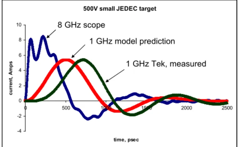
Figure 5 shows a sequence of three waveforms taken at Intel (A. Daniel, M. Farris) on a Thermo CDM tester with the JEDEC test head and a small JEDEC target, 500V. The 8 GHz Tek scope waveform is at left; next is that waveform as filtered by the 1 GHz Tek impulse response (Fig. 3), and finally an actual measured 1 GHz waveform, delayed by 140 psec for clarity. For the 1 GHz waveforms, timing is good and peak currents (5.4 amp) match to <1% accuracy. Since the 500V air discharge CDM measurements were separate zaps for the 1 GHz and 8 GHz scopes, the total charge (integrated current to several nsec) was normalized to the 1 GHz Tek value, and thus the 8 GHz waveform scaled up by about 12%. The effective capacitance of the target as measured by the 1 GHz Tek scope on the CDM tester at 500V was 4.64 pF. This familiar value agrees with how the small JEDEC target of nominal 6.8 pF (through the dielectric) is modified by the series-parallel
Fast step plus filter
0 0.2 0.4 0.6 0.8 1 1.2
0 200 400 600 800 1000 1200 1400
time, psec
N
o
rm
al
iz
ed
vo
lt
s
1G data
8G data + filter Fast step plus filter
0 0.2 0.4 0.6 0.8 1 1.2
0 200 400 600 800 1000 1200 1400
time, psec
N
o
rm
al
iz
ed
vo
lt
s
1G data
with the 3-capacitor model [12,13] of the CDM tester.
Figure 5. 8 GHz CDM waveform and its convolution with 1GHz Tek impulse response model (Fig. 3), then compared with (delayed) 1 GHz Tek CDM waveform taken under the same conditions.
Note how the small JEDEC CDM target waveforms have high-frequency content that is readily seen on a fast scope, but is washed out when the CDM measurement channel is lower frequency. It is unfortunate that the integrated current (charge) had to be forced to be the same, but air discharge CDM can often vary at this level among pulses taken at the same voltage. These scopes were all within 1% of each other in the steady value of the step response, so they do function well as fast voltmeters. Future experiments could check their behavior as fast electrometers, for example using a high-bandwidth resistive splitter to send a CDM pulse to two scopes at once, or calibrating to a known impulse generator as well as to a step generator. Some impulse generators on the market [14] could provide a known high-speed charge packet for calibration at CDM time scales.
Figure 6. 8 GHz CDM waveform, then filtered by 1 GHz Agilent 2-pole FIR model. Measured waveform (delayed) matches predicted peak current within 1%.
Figure 6 shows the same waveforms and application of the filter model, but for the slightly faster (see Table I) Agilent scope. Again the waveforms were scaled to normalize charge to 2.32 nC (4.64 pF) as measured by integrated current. This was about a 4% downward adjustment, quite possibly because of the unique zap recorded for the Agilent scope. The Agilent waveform also had an obvious offset of about 40 mV (corresponding to 40 mA) which had to be removed—offsets can be a larger problem for the time scale of HBM waveforms [3,4], but even at the CDM time scale one should look for effects on current integration and subtract out the background offset.
IV. Application to TLP
Transients
The above concepts about filters can be applied to the time-dependent properties of devices as tested by TLP. The non-ideal step function V0(s), again with the an series, is applied, with output impedance Z0, and voltage across the device (Z(s)=1/Y(s)) is measured (Figure 7). If the device’s dc resistance is R1=1/Y1, and the device admittance is Y(s)=Y1(1+d1s+d2s2+…)=1/Z(s), then the measured device voltage is
...) 1 ( 1 ) ( ) ( 2 2 1 1 0 0 s d s d Y Z s V s VD ... 1 ... 1 1 / 2 2 1 2 2 1 1 0 0 s b s b s a s a Y Z s V
, (16)
where 0 1 0 1 1 1
/
1
,
/
1
R
Z
d
b
Z
R
d
b
nn
.The normalization factor out front in (16) is of course the voltage division relation that is the usual focus of TLP in the steady state. The rest of (16) is amenable to applying Eq. (3) to determine b1,b2… after finding a1,a2… from TLP calibration with a matched load. The transient behavior of Z(s) or Y(s) is thus reducible to filter parameters through successive integration, with no particular limit on the order of the network. The comparable expression for the device current in terms of Z(s)=R1(1+f1s+f2s2+…)=1/Y(s) is
2 2 1 2 2 1 1 0 0 1 1 / ) ( s c s c s a s a R Z s V s
ID , (17)
where 1 0 1 0 1 1
/
1
,
/
1
Z
R
f
c
R
Z
f
c
nn
.500V small JEDEC target
-4 -2 0 2 4 6 8 10
0 500 1000 1500 2000 2500
time, psec cu rr en t, A m p s
8 GHz scope
1 GHz Tek, measured 1 GHz model prediction
500V small JEDEC target
-4 -2 0 2 4 6 8 10
0 500 1000 1500 2000 2500
time, psec cu rr en t, A m p s
8 GHz scope
1 GHz Tek, measured 1 GHz model prediction
500V CDM JEDEC small target
-4 -2 0 2 4 6 8 10
0 500 1000 1500 2000 2500
time, psec cu rr ent , A m ps
8 GHz scope
1 GHz Agilent, measured 1 GHz model prediction
500V CDM JEDEC small target
-4 -2 0 2 4 6 8 10
0 500 1000 1500 2000 2500
time, psec cu rr ent , A m ps
8 GHz scope
The cn series will result from successive integration of ID(t), with adjustment for the source series an, per Eq. (3). For small R1, which is common, the impedance coefficients fn will have a much larger multiplier and be much more sensitive to source rise time (minus) a1, and so on. But in the end, the Z(s) and Y(s) series should be redundant, and Eq. (3) tells us that f1=-d1.
Figure 7. Transmission line pulse measurement network; device Z(s)=1/Y(s). Voltage is measured across Z(s).
Let us now apply this to an example of silicon-controlled rectifier (SCR) turn-on from previous work [15], where the author (R. Ashton) has kindly provided the raw data. A 50-ohm TLP source of about 20V open circuit was applied, producing turn-on of the SCR around 16V, and steady-state voltage of about 3.0V, with steady state current around 325 mA. For Figures 8 and 9, the steady-state voltages and currents were normalized to unity, in accordance with Eqs. (3), (16) and (17), so that coefficients could be easily extracted through integration and area capture.
Figure 8. Normalized SCR voltage transient and scaled generating step, from [15]. The captured area between them gives the first term b1 as in Eq. (16) and accounts for the step
delay a1.
In Fig. 8, we know from the discussion leading up to Eq. (3) that (a1-b1) is the (normalized) SCR voltage integral after the unit step height has been
subtracted. This will have positive and negative components, but to find b1 next, the (negative) value of a1, the Elmore Delay of the step, about 6.9 nsec, needs to be removed. The result of adding and subtracting those areas is that b1, negative because of the overshoot, is found by measuring the area between the overshooting SCR voltage and the scaled step waveform. Don’t forget that the actual step voltage must always exceed the SCR voltage; it is scaled here because the geometric meaning of a1 [3-6, 8] is thereby expressed for the sake of the area calculation. The Y(s) coefficient d1 is then calculated by multiplying b1 by 1.175, as R1 is 8.75 ohms, and is around (minus) 41.5 nsec.
Figure 9. Normalized SCR current transient and scaled generating step, from [15]. The captured area between them gives the first term c1 as in Eq. (17) and accounts for the step
delay a1.
A similar situation arises for the SCR current transient, as seen in Fig. 9 and relating to Eq. (17). This time (a1-c1) for Z(s) results from the (normalized) current integral after the unity offset is removed. Because the step lies above the SCR curve, c1 is positive, also consistent with an inductive impedance. Because R1=8.75 ohms, there is a much higher multiplier for c1 to get Z(s) coefficient f1, as we stated before. The sensitivity to the generating step, claimed earlier following Eq. (17), is graphically seen in Fig. 9; note how much less sensitive to the step properties the Fig. 8 area is. Even so, f1 matched -d1 exactly at 41.5 nsec given a preferred choice for step delay a1 within 5% of all “reasonable” values. The Z(s) and Y(s) methods for measuring the first-order transient properties of this SCR are thus found to be equivalent and redundant, as expected.
The above process extracts a single scalar time constant to characterize a device transient, and could be extended to more series terms if desired.
V
0(s)
Z(s)
Z
0First Y(s) term, SCR
0 1 2 3 4 5 6
0 5 10 15 20 25
time, nsec
N
o
rm
al
iz
ed
vo
lt
ag
e
step SCR voltage
-b1=Area
First Y(s) term, SCR
0 1 2 3 4 5 6
0 5 10 15 20 25
time, nsec
N
o
rm
al
iz
ed
vo
lt
ag
e
step SCR voltage
-b1=Area
First Z(s) term, SCR
0 0.2 0.4 0.6 0.8 1 1.2
0 5 10 15 20 25
time, nsec
N
o
rm
al
iz
ed
c
u
rre
nt
step
SCR current c1=Area
First Z(s) term, SCR
0 0.2 0.4 0.6 0.8 1 1.2
0 5 10 15 20 25
time, nsec
N
o
rm
al
iz
ed
c
u
rre
nt
step
It is a bit involved, but in the end, the procedure is clear enough that one can easily imagine computer software to make fast work of time constant extraction, given some digital waveforms. With time constants easily accessible along with steady-state I-V, we can more easily examine device trends as we change, for example, the voltage, impedance, or rise time of the TLP source. New device insights are almost certain if we have this method, implemented in software, to examine transients in diodes, snapback devices, and SCRs. The algorithm could be coded as part of a university project or as part of code development in support of commercial TLP systems. Eventually, transient TLP data, at least to first order, should become as familiar to users as steady-state I-V curves, and users will likely find applications for it that are unknown today.
V. Conclusions
It is now possible to characterize and model oscilloscopes used for CDM measurements more simply than ever. The filtering of high frequency information in the CDM waveform can be anticipated through careful examination of the fast step response of the scope, whereupon the 10-90% rise time, easily measured, leads to a two-pole FIR filter model. This has precedents in an earlier study of nine different oscilloscopes [7], but in this work the soundness of the method is cross-checked with moment-matching methods [3-6, 8]. Also, we use convolution algorithms [11] to apply the filter models to high-frequency (8 GHz) CDM data, and successfully reproduce the measured waveforms with lower-frequency (1 GHz) scopes. The simple 2-pole model with D=0.707, obtained immediately from 10-90% rise times, was remarkably effective as a final filter model, but it was important to confirm that the various scopes were serving as (1) good high-speed voltmeters for step response, and (2) good high-speed electrometers for measuring equal charge (current integral) for the same pulse. Further work on (2) would be helpful, and impulse generators may join the step generators in calibration of the scopes.
The 2-pole filter models reproduce some but not all features of the measured steps, although they anticipate the ultimate CDM peak current and general waveform shape extremely well. If desired, fast “startup poles” could augment the 2-pole model for a smooth starting derivative, or perhaps a Gaussian impulse could be convolved with a ringing 2-pole step, to introduce Gaussian startup
smoothness while preserving some of the observed step overshoot.
Nonetheless, 2-pole FIR filters, extracted as described herein, are probably sufficient for specifying new CDM waveform standards. These elements should be present:
1. A starting CDM waveform for the calibration target (small JEDEC has the most high-frequency content) at high frequency, or “unfiltered”, should be specified, analytically or numerically. 2. A 2-pole FIR filter model, appropriate to
the scope being used, is applied to this CDM standard waveform to set peak current and pulse width expectations for the target scope. The current integral (charge) expectations, i.e., effective target capacitance, should also be stated.
3. High-frequency scopes (e.g., 8 GHz) need not reproduce all features of the “standard” waveform, but as they usually include built-in filters, those filters (or external hardware filters) will be fit to the 2-pole model and the “simplified” waveform properties and expectations used.
Looking forward, the existing 1 GHz scopes will give way to 3 GHz and higher frequency scopes; in agreement with [1] it is probably best to be capable of at least 3 GHz in the CDM lab. Even so, this work shows that the well-understood 1 GHz scope can still be very useful in CDM checks, and reconcilable with similar scopes. These simple high-speed calibration measurements usually explain discrepancies very effectively, and allow more equipment to be used with confidence.
single time constant accompanying each steady-state I-V point, and easily accessed from digital data, would help the TLP user gain new insights into device behavior.
Acknowledgements
The authors thank Marti Farris of Intel, Marty Johnson of National Semiconductor, and Nathan Jack of Intel and UIUC, for waveforms taken in the early stages of this work. Robert Ashton of ON Semiconductor prepared and provided the SCR data for Section IV.
References
[1] T. Smedes, et al., “Pitfalls for CDM Calibration Procedures”, 2010 EOS/ESD Symposium, pp. 341-348.
[2] Web article, “LTI System Theory”,
http://en.wikipedia.org/wiki/LTI_system_theor y, and references cited therein.
[3] Timothy J. Maloney, “Evaluating TLP Transients and HBM Waveforms”, EOS/ESD Symposium Proceedings, pp. 143-151, 2009. [4] Timothy J. Maloney, “HBM Waveforms,
Equivalent Circuits, and Socket Capacitance”, EOS/ESD Symposium Proceedings, pp. 407-415, 2010.
[5] W.C. Elmore, “The Transient Analysis of Damped Linear Networks With Particular Regard to Wideband Amplifiers”, J. Appl. Phys. Vol. 19(1), pp. 55-63 (1948).
[6] R. Gupta, B. Tutuianu, and L.T. Pileggi, “The Elmore Delay as a Bound for RC Trees with Generalized Input Signals”, IEEE Trans. on Computer-Aided Design of Integrated Circuits
and Systems, vol 16, no. 1, pp. 95-104, January 1997.
[7] C. Mittermayer and A. Steininger, "On the Determination of Dynamic Errors for Rise Time Measurement with an Oscilloscope", IEEE Trans. on Instrumentation and Measurement, Vol. 48, no. 6, pp. 1103-07, Dec. 1999.
[8] Y.I. Ismail, E.G. Friedman, and J.L. Neves., “Equivalent Elmore Delay for RLC Trees”, ACM Design Automation Conference, 1999. [9] R.N. Bracewell, The Fourier Transform and Its
Applications, (New York: McGraw-Hill, 1965).
[10] M. Abramowitz and I.A. Stegun, Handbook of Mathematical Functions, New York: Dover Publications, 1965.
[11] Web resource, “Excellaneous” VB macros, at
http://www.bowdoin.edu/~rdelevie/excellaneou s/#downloads.
[12] R. Renninger, M-C. Jon, D.L. Lin, T. Diep and T.L. Welsher, “A Field-Induced Charged-Device Model Simulator”, EOS/ESD Symp. pp. 59-71, 1989.
[13] J.A. Montoya and T.J. Maloney, “Unifying Factory ESD Measurements and Component ESD Stress Testing”, EOS/ESD Symp. pp. 229-237, 2005.
[14] Picosecond Pulse Labs; web page at
http://www.picosecond.com.
[15] R. Ashton, "Extraction of Time Dependent Data from Time Domain Reflection Transmission Line Pulse Measurements", International Conference on Microelectronic Test Structures, 2005, pp. 239-44.


![Figure 9. Normalized SCR current transient and scaled generating step, from [15]. The captured area between them gives the first term c 1 as in Eq](https://thumb-us.123doks.com/thumbv2/123dok_us/8195200.2172550/7.918.87.457.693.924/figure-normalized-current-transient-scaled-generating-captured-gives.webp)
