ADAPTIVE MODELING OF DETAILS FOR PHYSICALLY-BASED SOUND SYNTHESIS AND PROPAGATION
Hengchin Yeh
A dissertation submitted to the faculty of the University of North Carolina at Chapel Hill in partial fulfillment of the requirements for the degree of Doctor of Philosophy in the Department of
Computer Science.
Chapel Hill 2014
ABSTRACT
HENGCHIN YEH: Adaptive Modeling of Details for Physically-based Sound Synthesis and Propagation
(Under the direction of Ming C. Lin)
In order to create an immersive virtual world, it is crucial to incorporate a realistic aural experience that complements the visual sense. Physically-based sound simulation is a method to achieve this goal and automatically provides audio-visual correspondence. It simulates the physical process of sound: the pressure variations of a medium originated from some vibrating surface (sound synthesis), propagating as waves in space and reaching human ears (sound propagation). The perceived realism of simulated sounds depends on the accuracy of the computation methods and the computational resource available, and oftentimes it is not feasible to use the most accurate technique for all simulation targets. I propose techniques that model the general sense of sounds and their details separately and adaptively to balance the realism and computational costs of sound simulations.
ACKNOWLEDGEMENTS
The many years that I spent working in the Department of Computer Science at UNC Chapel Hill on the research projects that would finally lead to this dissertation have been a great journey. First and foremost, I would like to thank my advisor, Prof. Ming C. Lin, for her guidance and support, as well as the freedom that she granted me in exploring my research interest, and patience that she showed for every change of my research directions. I would also like to thank the members of my committee, Prof. Gary Bishop, Prof. Dinesh Manocha, Prof. Marc Niethammer, and Dr. Nikunj Raghuvanshi, for tgation.
I would also like to thank the collaborators I have had the honor of working with, including Zhimin Ren, Ravish Mehra, Lakulish Antani, Sean Curtis, Qi Mo, Will Moss, Jur van den Berg, and Sachin Patil. I would also like to thank Dr. Anish Chandak at Impulsonic Incorporation and Dr. Micah Taylor at Rose-Hulman Institute of Technology for their insight and help, and Dr. J. Rafael Tena at Disney Research for his guidance as my intern supervisor. I would also like to thank the many anonymous reviewers for helping me improve the quality of my work.
TABLE OF CONTENTS
LIST OF TABLES . . . xi
LIST OF FIGURES . . . xiii
1 INTRODUCTION . . . 1
1.1 Adaptive Modeling of Details . . . 2
1.2 Thesis Statement . . . 3
1.3 Challenges and Contributions . . . 4
1.3.1 Sound Simulation from Fluid Simulation . . . 4
1.3.2 Example-Guided Rigid Body Sound Synthesis . . . 5
1.3.3 Wave-Ray Hybrid Sound Propagation . . . 6
1.4 Thesis Organization . . . 8
2 PREVIOUS WORK . . . 9
2.1 Sound Synthesis . . . 9
2.1.1 Liquid Sounds . . . 9
2.1.2 Rigid Body Sounds . . . 10
2.1.2.1 Parameter Acquisition . . . 11
2.1.2.2 Modal Plus Residual Models . . . 13
2.2 Sound Propagation . . . 13
2.2.1 Numerical Acoustic Techniques . . . 14
2.2.2 Geometric Acoustic Techniques . . . 15
2.2.3 Hybrid Techniques . . . 15
3 SOUND SYNTHESIS FROM FLUID SIMULATION . . . 18
3.1 Liquid Sound Principles . . . 18
3.1.1 Spherical Bubbles . . . 18
3.1.2 Generalization to Non-Spherical Bubbles . . . 20
3.1.3 Statistical Generation . . . 25
3.1.3.1 Bubble Generation Criteria . . . 25
3.1.3.2 Bubble Distribution Model . . . 26
3.2 Integration with Fluid Dynamics . . . 27
3.2.1 Shallow Water Method . . . 27
3.2.1.1 Dynamics Equations . . . 27
3.2.1.2 Rigid Bodies . . . 29
3.2.2 Grid-SPH Hybrid Method . . . 30
3.2.2.1 Dynamics Equations . . . 30
3.2.2.2 Bubble Extraction . . . 31
3.2.2.3 Bubble Tracking and Merging . . . 31
3.2.2.4 Spherical Harmonic Decomposition . . . 32
3.2.3 Decoupling Sound Update from Graphical Rendering . . . 33
3.3 Implementation and Results . . . 33
3.3.1 Benchmarks . . . 34
3.3.1.1 Hybrid Grid-SPH Simulator . . . 34
3.3.1.2 Shallow Water Simulator . . . 36
3.3.2 Timings . . . 37
3.3.3 Comparison with Harmonic Fluids . . . 40
3.4 User Study . . . 41
3.4.1 Procedure . . . 42
3.4.2 Results . . . 43
3.4.2.1 Demographics . . . 45
3.4.2.3 Section I and II . . . 45
3.4.2.4 Our method vs. Single-Mode Approximation . . . 46
3.4.2.5 Roles of Audio Realism and AV Synchronization . . . 46
3.4.2.6 Analysis . . . 47
3.5 Conclusion, Limitations, and Future Work . . . 47
4 EXAMPLE-GUIDED RIGID BODY SOUND SYNTHESIS . . . 49
4.1 Background . . . 49
4.1.1 Modal Sound Synthesis: . . . 49
4.1.2 Material properties . . . 50
4.1.3 Constraint for modes . . . 51
4.2 Methodology . . . 51
4.3 Feature Extraction . . . 53
4.4 Parameter Estimation . . . 56
4.4.1 An Optimization Framework . . . 56
4.4.2 Metric . . . 58
4.4.2.1 Image Domain Metric . . . 59
4.4.2.2 Feature Domain Metric . . . 61
4.4.2.3 Hybrid Metric . . . 65
4.4.3 Optimizer . . . 66
4.5 Residual Compensation. . . 67
4.5.1 Residual Computation . . . 67
4.5.2 Residual Transfer . . . 68
4.5.2.1 Algorithm . . . 68
4.5.2.2 Implementation and Performance . . . 71
4.5.2.3 Constants and Functions . . . 71
4.6 Results and Analysis . . . 72
4.6.1.1 Comparison with Spectral Modeling Synthesis9 . . . 72
4.6.1.2 Comparison with a Phase Unwrapping Method . . . 74
4.6.2 Parameter estimation . . . 77
4.6.3 Comparison with real recordings . . . 79
4.6.4 Example: a complicated scenario . . . 79
4.6.5 Performance . . . 80
4.7 Conclusion and Future Work . . . 81
5 WAVE-RAY HYBRID SOUND PROPAGATION . . . 85
5.1 Overview . . . 85
5.1.1 Sound Propagation . . . 85
5.1.2 Acoustic Transfer Function . . . 86
5.1.3 Hybrid Sound Propagation . . . 87
5.2 Two-Way Wave-Ray Coupling . . . 89
5.2.1 Geometric→Numerical . . . 90
5.2.2 Numerical→Geometric . . . 91
5.2.3 Fundamental solutions . . . 92
5.2.4 Precomputed Transfer Functions . . . 94
5.3 Implementation . . . 97
5.3.1 Implementation details . . . 97
5.3.2 Collocated equivalent sources . . . 98
5.3.3 Auralization . . . 98
5.4 Results and Analysis . . . 99
5.4.1 Scenarios . . . 100
5.4.2 Error Analysis . . . 101
5.4.3 Complexity . . . 101
5.4.4 Comparison with Prior Techniques . . . 103
5.6 Extension to Inhomogeneous Media . . . 106
5.6.1 Ray Theory . . . 109
5.6.1.1 Solving the Eikonal Equation . . . 112
5.6.1.2 Solving the Transport Equation . . . 114
5.6.2 Dynamic Ray Tracing . . . 119
5.6.2.1 Phase Shift due to Caustics . . . 124
5.6.2.2 Ray Amplitudes . . . 125
5.6.3 Gaussian Beams . . . 125
5.6.4 Summation Methods . . . 127
5.6.4.1 Superposition Integrals . . . 127
5.6.4.2 Determination of the Weighting Function . . . 128
5.6.4.3 Travel-Time Function . . . 129
5.6.4.4 Specification of Matrix M . . . 131
5.6.4.5 Summation Methods: Discussion . . . 131
6 CONCLUSION AND FUTURE WORK . . . 133
LIST OF TABLES
3.1 Number of modes selected by the two criteria for various typicalr0’s.. . . 25
3.2 Hybrid Grid-SPH Benchmark Timings (seconds per frame).. . . 38
3.3 Shallow Water Benchmark Timings (msec per frame). . . 40
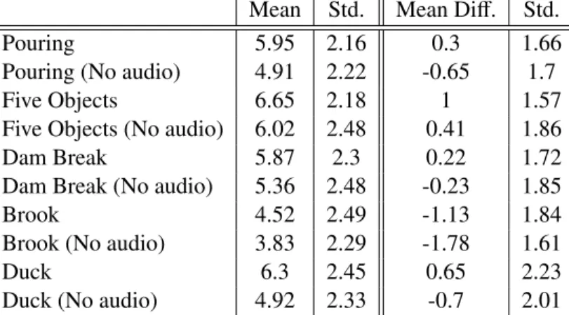
3.4 Section I Results: Audio Only. The means and standard deviations for section I. Column one is the mean score given by the subject, whereas, column three is the mean of the difference a given question’s score was from the mean score for this subject. We calculated this quantity in attempt to mitigate the problem of some subjects scoring all clips high and some subjects scoring all clips low. The top group represents the real sounds and the bottom group represents the sounds generated using our method.
All 97 subjects participated in this section. . . 43
3.5 Section II Results: Video vs. Visual Only. The means and standard deviations for section II. Column one is the mean score given by the subjects, whereas column three is the mean of the difference a given question’s score was from the mean score for this subject. A total of 87
out of 97 subjects chose to participated in this section. . . 43
3.6 Section III Results: Audio Only for Ours vs. Single-Mode. Columns one and two show the percentage (and absolute number) of people who found our videos to be the same or different than the minimal enclosing sphere method. Columns three and four show, of the people who said they were different, the percentage that preferred ours or the MES method and finally columns five and six show the mean of the stated strength of the preference for those who preferred our method and the MES method. A
total of 78 subjects participated in this section. . . 44
3.7 Section IV Results: Video for Ours vs. Single-Mode(top) & Ours vs. Recorded(bottom). The top group shows our method versus the minimal enclosing sphere method and the bottom group shows our method versus the prerecorded and synched sounds. Columns one and two show the percentage (and absolute number) of people who found the two videos to be the same or different. Columns three and four show, of the people who said they were different, the percentage that preferred ours or the other method (either MES or prerecorded) and finally columns five and six show the mean of the stated strength of the preference for those who preferred
our method and the other method. A total of 75 subjects participated in this section. . 44
4.1 Refer to Sec. 4.1 and Sec. 4.4 for the definition and estimation of these parameters. . . 78
5.1 Precomputation Performance Statistics. The rows “Building+small”, “Building+medium”, and “Building+large” correspond to scenes with a building surrounded by small, medium, and large walls, respectively. “Reservoir” and “Parking” denote the reservoir and underground parking
garage scene respectively. For a scene, “#src” denotes the number of sound sources in the scene, “#freq.” is the number of frequency samples, and “#eq. srcs” denotes the number of equivalent sources. The first part, “Hybrid Pressure Solving”. includes all the steps required to compute the final equivalent source strengths, and is performed once for a given sound source and scene geometries. The second part, “Pressure Evaluation”, corresponds to the cost of evaluating the contributions from all equivalent sources at a listener position and is performed once for each listener position. For the numerical technique, “wave sim.” refers the total simulation time of the numerical wave solver for all frequencies; “per-object” denotes the computation time of for per-object transfer functions; “inter-object” is the inter-object transfer functions for each pair of objects (including self-inter-object transfer functions, where the pressure wave leaves a near-self-inter-object region and reflected back to the same object); “source+global ” is the time to solve the linear system to determine the strengths of incoming and outgoing equivalent sources. For the geometric technique, “# tris” is the number of triangles in the scene; “order” denotes the order of reflections modeled; “# rays” is the number of rays emitted from a source (sound source or equivalent source). The column “prop. time” includes the time of finding valid propagation paths and computing pressures for any
intermediate step (e.g. from one object to another object’s offset surface). . . 96
5.2 Runtime Performance on a Single Core. For each scene, “#IR samples” denotes the number of IR’s sampled in the scene to support moving listen-ers or sources; “Memory” shows the memory to store the IR’s; “Time” is
the total running time needed to process and render each audio buffer. . . 99
5.3 Memory Cost Saving. The memory required to evaluate pressures at a given point of space. This corresponds to the same operation shown in the rightmost column of Table 5.1. Compared to standard numerical techniques, our method provides3 to 7 orders of magnitudeof memory
saving on the benchmark scenes. . . 104
LIST OF FIGURES
3.1 Here we show a simple bubble decomposed into spherical harmonics. The upper left shows the original bubble. The two rows on the upper right show the two octaves of the harmonic deviations from the sphere. Along the bottom is the sound generated by the bubble and the components for
each harmonic. . . 22
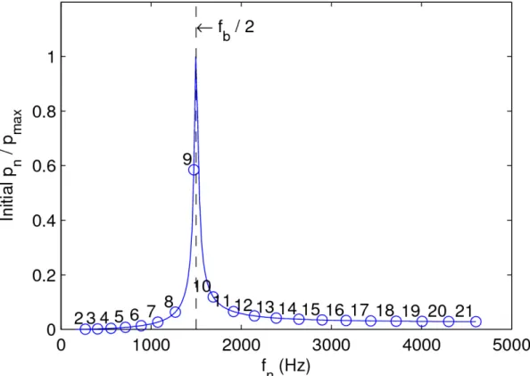
3.2 A plot of the initial amplitude vs. frequency. From the plot it is clear that as fn(the frequency of the bubble) approaches 12fb(the damping shifted
frequency) the initial amplitude increases dramatically. We, therefore, use harmonics where fn ≈ 12fbbecause they have the largest influence on the
initial amplitude. . . 24
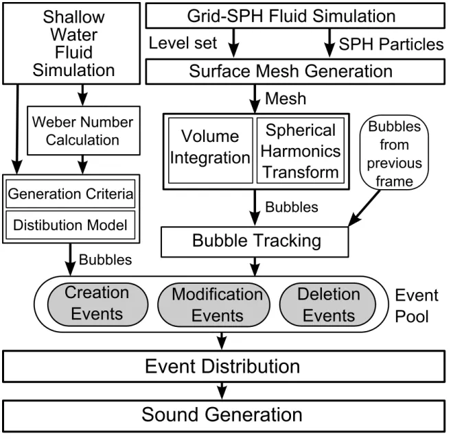
3.3 An overview of our liquid sound synthesis system . . . 28
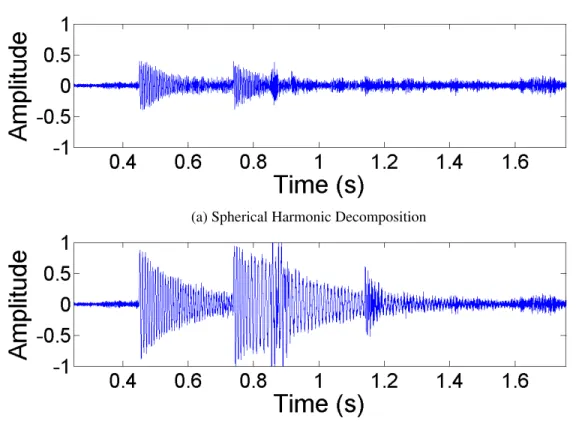
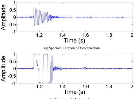
3.4 Wave plots showing the frequency response of the pouring benchmark. We have highlighted the moments surrounding the initial impact of the water and show our method (top) and a single-mode method (bottom) where the frequency for each bubble is calculated using volume of the minimum
enclosing sphere. . . 34
3.5 Liquid sounds are generated automatically from a visual simulation of
pouring water. . . 35
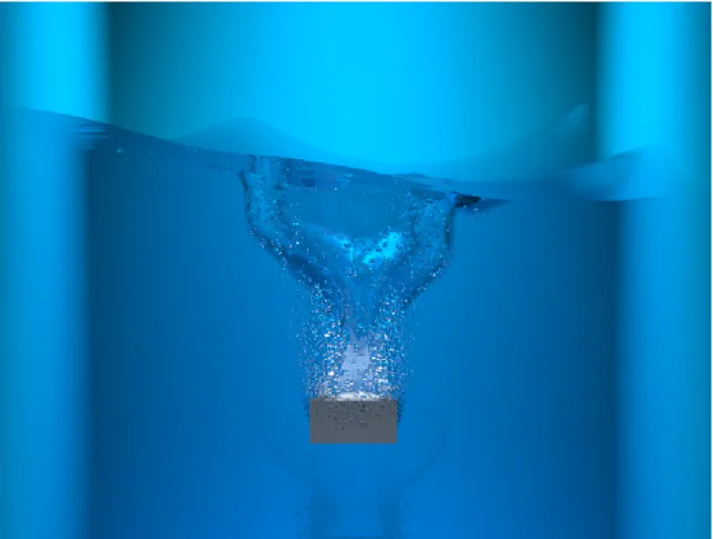
3.6 Wave plots showing the frequency response of the five objects bench-mark. We have highlighted the impact of the final, largest object. The top plot shows our method and the bottom, a single-mode method where the frequency for each bubble is calculated using volume of the minimum
enclosing sphere. . . 36
3.7 Sound is generated as five objects fall into a tank of water one after another. . . 37
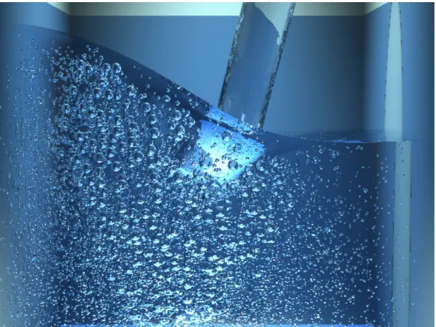
3.8 Wave plots showing the frequency response for the dam break scenario. We highlight the moment when the second wave crashes (from right to left) forming a tube-shaped bubble. The top plot shows our method and the bottom, a single-mode method where the frequency for each bubble is
calculated using volume of the minimum enclosing sphere. . . 38
3.9 A “dam-break” scenario, a wall of water is released, creating turbulent
waves and sound as the water reflects offthe far wall. . . 39
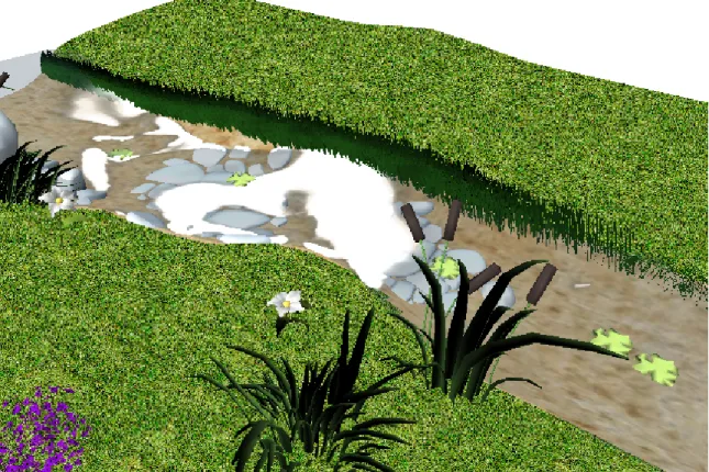
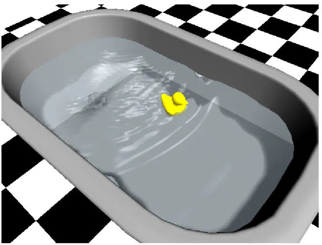
3.10 Real-time sounds are automatically generated from an interactive
simula-tion of a creek flowing through a meadow. . . 40
4.1 From the recording of a real-world object (a), our framework is able to find the material parameters and generates similar sound for a replicate object (b). The same set of parameters can be transfered to various virtual
objects to produce sounds with the same material quality ((c), (d), (e)). . . 52
4.2 Overview of the example-guided sound synthesis framework (shown in the blue block): Given an example audio clip as input, features are extracted. They are then used to search for the optimal material parameters based on a perceptually inspired metric. A residual between the recorded audio and the modal synthesis sound is calculated. At run-time, the excitation is observed for the modes. Corresponding rigid-body sounds that have a sim-ilar audio quality as the original sounding materials can be automatically synthesized. A modified residual is added to generate a more realistic final
sound. . . 53
4.3 Feature extraction from a power spectrogram. (a) A peak is detected in a power spectrogram at the location of a potential mode. f=frequency, t=time. (b) A local shape fitting of the power spectrogram is performed to estimate the frequency, damping and amplitude of the potential mode. (c) If the fitting error is below a certain threshold, we collect it in the set of extracted features, shown as the red cross in the feature space. (Only the
frequency f and dampingdare shown here.) . . . 55 4.4 Psychoacoustics related values: (a) the relationship between
critical-band rate (in Bark) and frequency (in Hz); (b) the relationship between loudness levelLN(in phon), loudnessL(in sone), and sound pressure level
Lp(in dB). Each curve is anequal-loudness contour, where a constant
loudness is perceived for pure steady tones with various frequencies. . . 60
4.5 Different representation of a sound clip. Top: time domain signals[n]. Middle: original image, power spectrogramP[m, ω] with intensity mea-sured in dB. Bottom: image transformed based on psychoacoustic prin-ciples. The frequency f is transformed to critical-band rate z, and the intensity is transformed toloudness. Two pairs of corresponding modes are marked as A and B. It can be seen that the frequency resolution decreases toward the high frequencies, while the signal intensities in both the
higher-and lower-end of the spectrum are de-emphasized. . . 62
4.6 Point set matching problem in the feature domain: (a) in the original frequency and damping, (f,d)-space. (b) in the transformed, (x,y)-space, wherex = X(f) andy =Y(d). The blue crosses and red circles are the reference and estimated feature points respectively. The three features
4.7 Residual computation. From a recorded sound (a), the reference features are extracted (b), with frequencies, dampings, and energies depicted as the blue circles in (f). After parameter estimation, the synthesized sound is generated (c), with the estimated features shown as the red crosses in (g), which all lie on a curve in the (f,d)-plane. Each reference feature may be approximated by one or more estimated features, and its match ratio number is shown. The represented sound is the summation of the reference features weighted by their match ratios, shown as the solid blue circles in (h). Finally, the difference between the recorded sound’s power spectrogram (a) and the represented sound’s (d) are computed to obtain
the residual (e). . . 69
4.8 Single mode residual transform: The power spectrogram of a source mode (f1,d1,a1) (the blue wireframe), is transformed to a target mode (f2,d2,a2) (the red wireframe), through frequency-shifting, time-stretching, and height-scaling. The residual power spectrogram (the blue surface at the bottom) is transformed in the exact same way. . . 71
4.9 Estimation of damping value in the presence of noise, using (a) our local shape fitting method and (b) SMS with linear regression. . . 73
4.10 Average damping error versus damping value for our method and SMS. . . 74
4.11 Interference from a neighboring mode located several bins away. . . 75
4.12 A noisy, high damping experiment. . . 75
4.13 Results of estimating material parameters using synthetic sound clips. The intermediate results of the feature extraction step are visualized in the plots. Each blue circle represents a synthesized feature, whose coordinates (x,y,z) denote the frequency, damping, and energy of the mode. The red crosses represent the extracted features. The tables show the truth value, estimated value, and relative error for each of the parameters. . . 77
4.14 Parameter estimation for different materials. For each material, the mate-rial parameters are estimated using an example recorded audio (top row). Applying the estimated parameters to a virtual object with the same geom-etry as the real object used in recording the audio will produce a similar sound (bottom row). . . 78
4.16 Transfered material parameters and residual: from a real-world recording (a), the material parameters are estimated and the residual computed (b). The parameters and residual can then be applied to various objects made of the same material, including (c) a smaller object with similar shape; (d) an object with different geometry. The transfered modes and residuals are
combined to form the final results (bottom row). . . 80
4.17 Comparison of transfered results with real-word recordings: from one recording (column (a), top), the optimal parameters and residual are es-timated, and a similar sound is reproduced (column (a), bottom). The parameters and residual can then be applied to different objects of the same material ((b), (c), (d), bottom), and the results are comparable to the
real-world recordings ((b), (c), (d), top). . . 81
4.18 The estimated parameters are applied to virtual objects of various sizes and shapes, generating sounds corresponding to all kinds of interactions
such as colliding, rolling, and sliding. . . 81
5.1 Overview of spatial decomposition in our hybrid sound propagation tech-nique: In the precomputation phase, a scene is classified into objects and environment features. This includes near-object regions (shown in orange) and far-field regions (shown in blue). The sound field in near-object re-gions is computed using a numerical wave simulation, while the sound field in far-field region is computed using geometric acoustic techniques. A two-way coupling procedure couples the results computed by geometric and numerical methods. The sound pressures are computed at different listener positions to generate the impulse responses. At runtime, the pre-computed impulse responses (IR0-IR3) are retrieved and interpolated for
the specific listener position (IRt) at interactive rates, and final sound is
rendered. . . 86
5.2 Frequency and spatial decomposition. High frequencies are simulated using geometric techniques, while low frequencies are simulated using a combination of numerical and geometric techniques based on a spatial
decomposition. . . 87
5.3 Two-way coupling of pressure values computed by geometric and numeri-cal acoustic techniques. (a) The rays are collected at the boundary and the pressure evaluated. (b) The pressure on the boundary defines the incident pressure fieldpincinΩN, which serves as the input to the numerical solver.
(c) The numerical solver computes the scattered fieldpsca, which is the
effect of objectAto the pressure field. (d)pscais expressed as fundamental
solutions and represented as rays emitted toΩG. . . 89
5.4 Our hybrid technique is able to model high-fidelity acoustic effects for large, complex indoor or outdoor scenes at interactive rates: (a) building surrounded by walls, (b) underground parking garage, and (c) reservoir
5.5 Comparison between the magnitude of the total pressure field computed by our hybrid technique and BEM for various scenes. In the top row, the red dot is the sound source, and the blue plane is a grid of listeners. Errors between our method and BEM for each frequency are shown in each row. For our hybrid technique, the effect of the two walls are simulated by numerical acoustic techniques, and the interaction between the ground or the room is handled by geometric acoustic techniques. For BEM, the entire scene (including the walls, ground, and room) is simulated together. The last column also shows comparison with a pure geometric technique
(marked as “GA”). . . 105
5.6 Error||Pref−Phybrid||2/||Pref||between the reference wave solver (BEM) and
our hybrid technique for varying maximum order of reflections modeled. The tested scene is the ”Two walls in a room” (see also Figure 5.5, last
column). . . 106
5.7 Breakdown of Precomputation Time. For a building placed in terrains of increasing volumes (small, medium, and large walls), the yellow part is the simulation time for the numerical method, and the green part is for the geometric method. The numerical simulation time scales linearly to the
largest dimension (L) of the scene instead of the total volume (V). . . 107
5.8 Initial take-offanglesi0andφ0as ray parameters. i0is the angle between
the ray direction and the x3-axis, whileφ0is the angle between the ray
direction and the x1-x3plane. 0≤ i0 ≤ πand 0 ≤ φ0 < 2π. A possible
choice of the initial basis vectors~e1,~e2,~e3of the ray-centered coordinate
system are also plotted on the unit sphere. . . 114
5.9 Basis vectors~e1,~e2,~e3of the ray-centered coordinate systemqiconnected
with rayΩ. RayΩis theq3-axis of the system. At any point on the ray, unit vector~e3equals~t, the unit tangent toΩ. Unit vectors~e1 and~e2 are
perpendicular toΩand are mutually perpendicular. . . 115
5.10 Ray tube. RayA0Acorresponds to ray parameters (γ1, γ2), rayB0B corre-sponds to (γ1+dγ1, γ2), rayC0Ccorresponds to (γ1+dγ1, γ2+dγ2), and
rayD0Dcorresponds to (γ1, γ2+dγ2). . . 117
5.11 Two types of caustic points. At a caustic point of the first order (a), the ray tube reduces to an arc. At a caustic point of the second order (b), the ray
tube shrinks to a point. . . 118
5.12 Computing ˆHalong the rayΩ. ˆHis determined by the basis vectors~e1,
~e2, and~e3of the ray-centered coordinate system. For a ray lying on plane Σ∥, I may define a set of unit vectors~n1,~n2,~n3 =~t. ~n2is chosen to be
perpendicular toΣ∥. The evolution of~ei follows~ni, where the angleθ0
5.13 Approximation of the wave field atRas a weighted sum of contributions from nearby Gaussian beams. Two Gaussian beams connected to ray Ω(γ1, γ2) andΩ(γ10, γ20) are shown, where pointsRγandRγ0close toR(not
CHAPTER 1: INTRODUCTION
In our real-world experience, we are constantly submerged in a wide variety of sounds. The auralexperience complements the visual sense. For example, when we see a wave crashing on a beach we expect to hear the splashing sound. When we walk toward talking people we expect to hear them more clearly, and the voice should become less distinctive when we walk around a corner. In a virtual environment, being able to incorporate sound effects that corresponds to visual events greatly enhances users’ immersion. Sound effect production thus has a wide application in video games, computer animation, films, training systems, computer aided design, scientific visualization, and assistive technology for the visually impaired.
Traditional methods of incorporating sound effect is a laborious practice. talented Foley artists are normally employed to record a large number of sound samples in advance and manually edit and synchronize the recorded sounds to a visual scene. This approach generally achieves satisfactory results. However, it is labor-intensive and cannot be applied to all interactive applications. It is still challenging, if not infeasible, to produce sound effects that precisely capture complex interactions
that cannot be predicted in advance.
Thereforephysically-based sound simulationhas been developed as a method to automatically integrate sounds into a virtual environment. It aims to simulate the physical process of sound, which is essentially the pressure variations of a medium originated from some vibration of surface, propagating in space and reaching human ears. Recent progress has been made on sound synthesis models that automatically produce sounds for various types of objects and phenomena. The practice directly provides audio-visual correspondence – it generates sounds that automatically synchronize with visual events and naturally capture the variation of object interactions (e.g. a ball bouncing or rolling, water in a brook running rapidly or calmly) or acoustic effects (e.g. the muffling of sound
Besides audio-visual correspondence, another factor is the quality of audio. In theory, if the perfect model of a physical phenomenon exists and infinite computing power is available, the resulting sound can be faithfully simulated from first principles. In practice, one model does not fit all. In some cases the existing model is not complete. For example, a universal damping model that can explain the vibration and sound-generating behavior of all materials is still an open research problem. In some cases the fine-scale dynamics is not resolved, especially when sound is to be generated from existing visual simulation. For example the fluid simulation in games usually provides only the surface information, and only in a coarse time resolution (30-60 fps). Even if an accurate model exists and all scales are resolved, the computational cost might be prohibitively high. On the other hand, simply omitting details and applying only coarse approximation often produces unsatisfactory results. Human ears are extremely sensitive to details: the ‘crisp’ noise of placing a coffee cup on a plate, the subtle variation of each rain drop, the acoustical quality of a concert hall – all contribute to perceived realism. A poorly simulated audio sounds ‘fake’ and affects the sense of immersion.
1.1 Adaptive Modeling of Details
In order to efficiently produce faithful aural experience for a complex sound source or
environ-ment, I propose techniques that model the general sense of sounds and their details separately. The principle is to first employs simplified, efficient methods to produce sounds that coarsely approximate the simulated sound sources (e.g. water motion, solid objects collision) or give a rough sense of the environment (e.g. a room or an open scene). Then rich and complex details are modeled separately and coupled into the system to improve realism of generated audios in an adaptive, user-controllable manner. The goal of my thesis is to develop simulation approaches that follow this general principle for many sound-related problems that are of interest to virtual environment applications.
For synthesizing liquid sounds, we adaptively model bubbles in different levels of details, because
decomposed into spherical harmonics, and the sound from each harmonic is summed. By choosing which bubbles are statistically generated, which bubbles are explicitly tracked, and which bubbles’ shapes are decomposed to spherical harmonics (and to what order), a user can control the trade-offs between realism and computational cost.
For synthesizing rigid-body contact sounds, linear modal synthesis is a powerful tool to simulate rigid-body sound in a physically-based manner, but the synthesized sounds are not as rich and realistic as real-world recordings. Recorded sounds, on the other hand, include a lot of details that linear modal synthesis does not model, such as fine-scale inhomogeneity, nonlinear resonant modes, and transient noise of unknown nature, are are still widely used in movies, animations, and games. I propose to improve the realism of linear modal synthesis in two levels. First, using an example recording to estimate the material parameters allows modal-synthesized sounds to preserve the inherent quality of the recorded material. Secondly, the difference between the example recording and the modal-synthesized sound is computed, transfered to different geometries if necessary, and
added back to the final synthesized sound.
For simulating sound propagation in a large scene, the adaptive modeling of details is achieved by combining two different acoustic techniques. Traditionally, numerical acoustic technique are used to accurately model wave phenomena such as diffraction, interference, and scattering, but
these techniques are generally expensive. Performing an accurate wave simulation for the entire scene, however, is usually not necessary – sound wave traveling in empty space and reflecting from large objects can be more efficiently modeled as rays with geometric acoustic techniques. Only in the vicinity of objects smaller than the wavelength of the sound waves are the wave phenomena significant and numerical techniques required. I propose to decompose the spatial domain of a scene and apply the numerical acoustic techniques only in limited, smaller regions, allowing a user to allocate computation resources on where it matters the most.
1.2 Thesis Statement
1.3 Challenges and Contributions
My contributions can be divided into three main areas, the simulation of liquid sounds, rigid-body contact sounds, and sound propagation. I will discuss the respective computational challenges as well as my contributions.
1.3.1 Sound Simulation from Fluid Simulation
I investigate new methods for sound synthesis in a liquid medium in the first part of my thesis. Our formulation is based on prior work in physics and engineering, which shows that sound is generated by the resonance of bubbles within the fluid (Rayleigh, 1917). We couple physics-based fluid simulation with the automatic generation of liquid sound based on Minneart’s formula (Minnaert, 1933) for spherical bubbles and spherical harmonics (Leighton, 1994) for non-spherical bubbles. We also present a fast, general method for tracking the bubble formations and a simple technique to handle a large number of bubbles within a given time budget.
The proposed synthesis algorithm offers the following advantages:
• It renders both liquid sounds and visual animation simultaneously using the same fluid simula-tor.
• It introduces minimal computational overhead on top of the fluid simulator.
• For fluid simulators that generates bubbles, no additional physical quantities, such as force, velocity, or pressure are required – only the geometry of bubbles.
• For fluid simulators without bubble generation, a physically-inspired bubble generation scheme provides plausible audio.
• It can adapt and balance between computational cost and quality.
1.3.2 Example-Guided Rigid Body Sound Synthesis
In real-time applications,modal synthesismethods are often used for simulating sounds. This approach generally does not depend on any pre-recorded audio samples to produce sounds triggered by all types of interactions, so it does not require manually synchronizing the audio and visual events. The produced sounds are capable of reflecting the rich variations of interactions and also the geometry of the sounding objects. Although this approach is not as demanding during run time, setting up good initial parameters for the virtual sounding materials inmodal analysisis a time-consuming and non-intuitive process. For a complicated scene consisting of many different sounding materials, the parameter selection procedure can quickly become prohibitively expensive and tedious.
Although tables of material parameters for stiffness and mass density are widely available, directly looking up these parameters in physics handbooks does not offer intuitive, direct control as using a recorded audio example. In fact, sound designers often record their own audio to obtain the desired sound effects. This chapter presents a new data-driven sound synthesis technique that
preserves the realism and quality of audio recordings, while exploiting all the advantages of physically based modal synthesis. We introduce a computational framework that takes just one example audio recording and estimates the intrinsicmaterial parameters(such as stiffness, damping coefficients, and mass density) that can be directly used in modal analysis.
As a result, for objects with different geometries and run-time interactions, different sets of modes are generated or excited differently, and different sounds are produced. However, if the material properties are the same, they should all sound like coming from the same material. For example, a plastic plate being hit, a plastic ball being dropped, and a plastic box sliding on the floor generate different sounds, but they all sound like ‘plastic’, as they have the same material
properties. Therefore, if we can deduce the material properties from a recorded sound andtransfer them to different objects with rich interactions, theintrinsic qualityof the original sounding material is preserved. Our method can also compensate the differences between the example audio and the modal-synthesized sound. Both the material parameters and the residual compensation are capable of being transfered to virtual objects of varying sizes and shapes and capture all forms of interactions.
• A feature-guided parameter estimation framework to determine the optimal material parameters that can be used in existing modal sound synthesis applications.
• An effective residual compensation method that accounts for the difference between the real-world recording and the modal-synthesized sound.
• A general framework for synthesizing rigid-body sounds that closely resemble recorded example materials.
• Automatic transfer of material parameters and residual compensation to different geometries and runtime dynamics, producing realistic sounds that vary accordingly.
1.3.3 Wave-Ray Hybrid Sound Propagation
Sound propagation techniques are used to model how sound waves travel in the space and interact with various objects in the environment. Sound propagation algorithms are used in many interactive applications, such as computer games or virtual environments, and offline applications, such as
noise prediction in urban scenes, architectural acoustics, virtual prototyping, etc.. Realistic sound propagation that can model different acoustic effects, including diffraction, interference, scattering,
and late reverberation, can considerably improve a user’s immersion in an interactive system and provides spatial localization (Blauert, 1983).
The acoustic effects can be accurately simulated by numerically solving the acoustic wave equation. Some of the well-known solvers are based on the boundary-element method, the finite-element method, the finite-difference time-domain method, etc. However, the time and space complexity of these solvers increases linearly with the volume of the acoustic space and is a cubic (or higher) function of the source frequency. As a result, these techniques are limited to interactive sound propagation at low frequencies (e.g. 1-2KHz) (Raghuvanshi et al., 2010; Mehra et al., 2013), and may not scale to large environments.
interference, and higher-order wave effects. Many hybrid combinations of numeric and geometric techniques have been proposed, but they are limited to small scenes or offline applications.
I have developed a novel hybrid approach that couples geometric and numerical acoustic techniques to perform interactive and accurate sound propagation in complex scenes. My approach uses a combination of spatial decomposition and frequency decomposition, along with a novel two-way wave-ray coupling algorithm. The entire simulation domain is decomposed into different
regions, and the sound field is computed separately by geometric and numerical techniques for each region. In the vicinity of objects whose sizes are comparable to the simulated wavelength (near-object regions), we use numerical wave-based methods to simulate all wave effects. In regions away from objects (far-field regions), including the free space and regions containing objects that are much larger than the wavelength, we use a geometric ray-tracing algorithm to model sound propagation. We restrict the use of numeric propagation techniques to small regions of the environment and precompute the pressure field at low frequencies. The rest of the pressure field is precomputed using ray tracing.
At the interface between near-object and far-field regions, we need to couple the pressures computed by the two different (one numerical and one geometric) acoustic techniques. Rays entering
a near-object region define the incident pressure field that serves as the input to the numerical acoustic solver. The numerical solver computes the outgoing scattered pressure field, which in turn has to be represented by rays exiting the near-object region. At the core of our hybrid method is a two-way coupling procedure that handles these cases. We present a scheme that represents two-way coupling usingtransfer functionsand computes all orders of interaction.
The key results of my work include:
• An efficient hybrid approachthat decomposes the scene into regions that are more suitable for either geometric or numerical acoustic techniques, exploiting the strengths of both.
• Fast, memory-efficient interactive audio renderingthat only uses tens to hundreds of megabytes of memory.
We have also tested our technique on a variety of scenarios and integrated our system with the Valve’s Source™game engine. Our technique is able to handle both large indoor and outdoor scenes (similar to geometric techniques) as well as generate realistic acoustic effects (similar to numeric wave solvers), including late reverberation, high-order reflections, reverberation coloration, sound focusing, and diffraction low-pass filtering around obstructions. Furthermore, our pressure evaluation takes orders of magnitude less memory compared to state-of-the-art wave equation solvers.
1.4 Thesis Organization
CHAPTER 2: PREVIOUS WORK
In this chapter I review related work in sound synthesis and sound propagation.
2.1 Sound Synthesis
In the last couple of decades, there has been strong interest in digital sound synthesis in both computer music and computer graphics communities due to the needs for auditory display in virtual environment applications. The traditional practice of Foley sounds is still widely adopted by sound designers for applications like video games and movies. Real sound effects are recorded and edited to match a visual display. More recently,granular synthesisbecame a popular technique to create sounds with computers or other digital synthesizers. Short grains of sounds are manipulated to form a sequence of audio signals that sound like a particular object or event. Roads (2004) gave an excellent review on the theories and implementation of generating sounds with this approach. Picard et al. (2009) proposed techniques to mix sound grains according to events in a physics engine.
Another approach for simulating sound sources isphysically based sound synthesis. Sounds of interesting natural phenomena as well as object interactions are simulated from physical principles, and the synthesized sounds automatically synchronize with the visual rendering. My work on sound synthesis follows this approach. I review the related work of physically-based simulation of liquid and rigid-body sounds, as well as work on improving realism of synthesized sound by acquiring parameters from real audio recordings and incorporating residuals.
2.1.1 Liquid Sounds
shallow-water approximations. We refer the reader to a recent survey (Bridson and M¨uller-Fischer, 2007) for more details.
For audio simulation, the physics literature presents extensive research on the acoustics of bubbles, dating back to the work of Lord Rayleigh (1917). There have been many subsequent efforts, including works on bubble formation due to drop impact (Pumphrey and Elmore, 1990;
Prosperetti and Oguz, 1993) and cavitation (Plesset and Prosperetti, 1977), the acoustics of a bubble popping (Ding et al., 2007), as well as multiple works by Longuet-Higgins presenting mathematical formulations for monopole bubble oscillations (1989b; 1989a) and non-linear oscillations (1991). T. G. Leighton’s (1994) excellent text covers the broad field of bubble acoustics and provides many of the foundational theories for my work.
Van den Doel (2005) introduced the first method in computer graphics for generating liquid sounds. Using Minneart’s formula, which defines the resonant frequency of a spherical bubble in an infinite volume of water in terms of the bubble’s radius, van den Doel provides a simple technique for generating fluid sounds through the adustment of various parameters. Other previous liquid sound synthesis methods provide limited physical basis for the generated sounds (Imura et al., 2007). Zheng and James integrated fluid simulation with bubble-based sound synthesis to automatically generate liquid sounds (2009). They consider spherical bubbles as in (van den Doel, 2005), and focus on the propagation of sound – both from the bubble to the water surface and the water surface to the listener. Their numerical sound propagation is compute-intensive and requires tens of hours of compute time on a cluster.
A related topic is simulating sound generated by air movement, which is also governed by fluid dynamics. Previous works include sound resulting from objects moving rapidly through air (2003) and the sound of woodwinds and other instruments (Florens and Cadoz, 1991; Scavone and Cook, 1998). Sound generated by the turbulent field due to fire has also been simulated (Dobashi et al., 2004; Chadwick and James, 2011).
2.1.2 Rigid Body Sounds
Their approach accurately captures surface vibration and wave propagation once sounds are emitted from objects. However, it is far from being efficient enough to handle interactive applications. Adrien (1991) introducedmodal synthesisto digital sound generation. For real-time applications, linear modal sound synthesishas been widely adopted to synthesize rigid-body sounds (van den Doel and Pai, 1998; O’Brien et al., 2002; Raghuvanshi and Lin, 2006; James et al., 2006a; Zheng and James, 2010). This method acquires a modal model (i.e. a bank of damped sinusoidal waves) using modal analysisand generates sounds at runtime based on excitation to this modal model. Moreover, sounds of complex interaction can be achieved with modal synthesis. Van den Doel et al. (2001) presented parametric models to approximate contact forces as excitation to modal models to generate impact, sliding, and rolling sounds. Ren et al. (2010) proposed including normal map information to simulate sliding sounds that reflect contact surface details.
More recently, Zheng and James (2011) created highly realistic contact sounds with linear modal synthesis by enabling non-rigid sound phenomena and modeling vibrational contact damping. The use of linear modal synthesis is not limited to creating simple rigid-body sounds. Chadwick et al. (2009) used modal analysis to compute linear mode basis, and added nonlinear coupling of those modes to efficiently approximate the rich thin-shell sounds. Zheng and James (2010) extended
linear modal synthesis to handle complex fracture phenomena by precomputing modal models for ellipsoidal sound proxies. Moreover, the standard modal synthesis can be accelerated with techniques proposed by (Raghuvanshi and Lin, 2006; Bonneel et al., 2008), which make synthesizing a large number of sounding objects feasible at interactive rates.
However, few previous sound synthesis work addressed the issue of how to determine material parameters used in modal analysis to more easily recreate realistic sounds.
2.1.2.1 Parameter Acquisition
parameter estimation. This method is capable of constructing a virtual sounding object that faithfully recreates the audible resonance of its measured real-world counterpart. However, each new virtual geometry would require a new measuring process performed on a real object that has exactly the same shape, and it can become prohibitively expensive with an increasing number of objects in a scene. This approach generally extracts hundreds of location-dependent parameters for one object from many audio clips, while the goal of our technique instead is to estimate only a few parameters that best represent onematerialof a sounding object from onlyoneaudio clip.
To the best of my knowledge, the only other research work that attempts to estimate sound parameters from one recorded clip is by Lloyd et al. (2011). Pre-recorded real-world impact sounds are utilized to find peak and long-standing resonance frequencies, and the amplitude envelopes are then tracked for those frequencies. They proposed using the tracked time-varying envelope as the amplitude for the modal model, instead of the standard damped sinusoidal waves in conventional modal synthesis. Richer and more realistic audio is produced this way. Their data-driven approach estimates the modal parameters instead of material parameters. Similar to the method proposed by Pai et al. (2001), these are per-mode parameters and not transferable to another object with corresponding variation. At runtime, they randomize the gains of all tracked modes to generate an illusion of variation when hitting different locations on the object. Therefore, the produced sounds
do not necessarily vary correctly or consistently with hit points. Their adopted resonance modes plus residual resynthesis model is very similar to that of SoundSeed Impact (Audiokinetic, 2011), which is a sound synthesis tool widely used in the game industry. Both of these works extract and track resonance modes and modify them with signal processing techniques during synthesis. None of them attempts to fit the extracted data (which are pre-object based) to estimate a higher-levelper-material basedmodel.
digital filters. They estimated the parameters for recursive filters based on pre-recorded audio and re-synthesized sounds in real time with digital audio processing techniques. This approach is not designed to capture rich physical phenomena that are automatically coupled with varying object interactions. The relationship between the perception of sounding objects and their sizes, shapes, and material properties have been investigated with experiments, among which Lakatos et al. (1997) and Fontana (2003) presented results and studied human’s capability to tell materials, sizes, and shapes of objects based on their sounds.
2.1.2.2 Modal Plus Residual Models
The sound synthesis model with a deterministic signal plus a stochastic residual was introduced to spectral synthesis by Serra and Smith (1990). This approach analyzes an input audio and divides it into a deterministic part, which are time-variant sinusoids, and a stochastic part, which is obtained by spectral subtraction of the deterministic sinusoids from the original audio. In the resynthesis process, both parts can be modified to create various sound effects as suggested by Cook (1996; 1997; 2002) and Lloyd et al. (2011). Methods for tracking the amplitudes of the sinusoids in audio dates back to Quateri and McAulay (1985), while more recent work (Serra and Smith III, 1990; Serra, 1997; Lloyd et al., 2011) also proposes effective methods for this purpose. All of these works directly construct the modal sounds with the extracted features. In contrast, our modal component is synthesized with the estimated material parameters. Therefore, although I adopt the same concept of modal plus residual synthesis for our framework, I face very different constraints due to the new
objective in material parameter estimation, and render these existing works not applicable to the problem addressed in my thesis.
2.2 Sound Propagation
2.2.1 Numerical Acoustic Techniques
Accurate, numerical acoustic simulations typically solve the acoustic wave equation using numerical methods. The Finite Difference Time Domain (FDTD) method was originally proposed
to model electromagnetic waves (Yee, 1966; Taflove and Hagness, 2005). It discretizes space as a uniform grid and solves for the field values at each cell for discrete time steps. It has been an adopted to room acoustics problems (Botteldooren, 1994, 1995) and has recently been applied to medium sized 3D scenes (Sakamoto et al., 2002, 2004, 2006). The Finite Element Method (FEM) (Zienkiewicz et al., 2006; Thompson, 2006) and the Boundary Element Method (BEM) (Cheng and Cheng, 2005; Gumerov and Duraiswami, 2009) discretize the scene’s volume and surface into elements respectively. They are usually employed to solve the steady-state frequency domain response, with FEM applied mainly to interior and BEM to exterior acoustic problems (Kleiner et al., 1993). Digital Waveguide Mesh approaches (Van Duyne and Smith, 1993) roots in musical synthesis and use discrete waveguide elements to propagate acoustic waves along a single dimension (Savioja, 1999; Karjalainen and Erkut, 2004; Murphy et al., 2007). Recently Raghuvanshi et al. proposed a method based on adaptive rectangular decomposition (2009a). It achieves high accuracy with a coarse spatial discretization.
These techniques, however, require the volume or boundary of the scene to be discretized at least twice the Nyquist frequency, and their time and space complexity increases as a third or fourth power of frequencies. Hence, these techniques often require many hours of simulation time and gigabytes of storage to model low frequencies in large scenes with static sources, and they scale as the third or fourth power of frequency. Despite recent advances, they remain impractical for many real-time applications.
2.2.2 Geometric Acoustic Techniques
Most acoustics simulation software and commercial systems are based on geometric tech-niques (Funkhouser et al., 1998; Vorlander, 1989) that assume sound travels along linear rays (Funkhouser et al., 2004). These methods are often based on stochastic ray tracing (Vorlander, 1989) or image sources (Borish, 1984). They frequently take advantage of recent advances in CPU- and/or
GPU-based ray tracing techniques (Taylor et al., 2009, 2012) or frustum tracing (Chandak et al., 2008; Lauterbach et al., 2007) to efficiently approximate sound propagation in complex, dynamic scenes.
The simplified assumption of rays limits these methods to accurately capture specular and diffuse reflections only at high frequencies. Diffraction is typically modeled by identifying individual diff ract-ing edges (Svensson et al., 1999; Tsract-ingos et al., 2001). These ray-based techniques can interactively model early reflections and first order edge-diffraction (Taylor et al., 2012); however, they cannot interactively model the reverberation of the impulse response explicitly, since that would require high-order reflections and wave effects such as scattering, interference, and diffraction. Hence,
many commercial systems approximate reverberation using the parameters of simple statistical models (Eyring, 1930).
While ray-tracing has been successfully used in many interactive acoustics systems (Lentz et al., 2007), the number of rays traced has to be limited for scenes with moving listeners in order to maintain real-time performance. As the worst-case complexity of image source methods scales exponentially with the number of polygons in the scene, some interactive systems often group the polygons to simplify the scene representation (Alarcao et al., 2010; Joslin and Magnenat-Thalmann, 2003).
2.2.3 Hybrid Techniques
Several methods for combining geometric and numerical acoustic techniques have been proposed. One line of work is based onfrequency decomposition: dividing the frequencies to be modeled into low and high frequencies. Low frequencies are modeled by numerical acoustic techniques, and high frequencies are treated by geometric methods, including the finite difference time domain
2012). However, these methods use numerical methods at lower frequencies over the entire domain. As a result, they are limited to offline applications and may not scale to very large scenes.
Another method of hybridization is based onspatial decomposition. The entire simulation domain is decomposed to different regions: near-object regions are handled by numerical acoustic techniques to simulate wave effects, while far-field regions are handled by geometric acoustic
techniques. Hampel et al. (2008) combine the boundary element method (BEM) and geometric acoustics using a spatial decomposition. Their method provides a one-way coupling from BEM to ray tracing, converting pressures in the near-object region (computed by BEM) to rays that enter the far-field region containing the listener. In electromagnetic wave propagation, Wang et al. (2000) propose a hybrid technique combining ray tracing and FDTD. Their technique is also based on a one-way coupling, where rays are traced in the far-field region and collected at the boundaries of the near-object regions. The pressures are then evaluated and serve as the boundary condition for the FDTD method. These one-way coupling methods do not allow rays to enter and exit the near-object regions of an object, and therefore acoustic effects of that object will not be propagated to the far-field
regions. Barbone et al. (1998) propose a two-way coupling that combines the acoustic field generated using ray-tracing and FEM. Jean et al. (2008) present a hybrid BEM/beam tracing approach to
compute the radiation of tyre noise. However, these methods do not describe how multiple entrance of rays into near-object regions of different objects is handled, which is crucial when simulating interaction between multiple objects.
2.2.4 Acoustic Kernel-Based Interactive Techniques
CHAPTER 3: SOUND SYNTHESIS FROM FLUID SIMULATION
In this chapter, I discuss my work on performing sound synthesis from fluid simulation. The rest of this chapter is organized as follows – in the next section I describe the physical principles of liquid sound. After that, I describe how liquid sound can be simulated by integrating various kinds of fluid simulators. Following this, I discuss the implementation details and the results obtained with my approach. Finally I conclude with a summary of my contributions and a discussion of limitations of my approach and possible directions of future work.
3.1 Liquid Sound Principles
Sound is produced by surface vibrations of an object under force(s). These vibrations travel through the surrounding medium to the human ear and the changes in pressure are perceived as sound. In the case of fluids, sound is primarily generated by bubble formation and resonance, creating pressure waves that travel though both the liquid and air media to the ear. Although an impact between a solid and a liquid will generate some sound directly, the amplitude is far lower than the sound generated from the created bubbles. We refer the reader to Leighton’s (1994) excellent text on bubble acoustics for more detail, and present an overview of the key concepts below.
3.1.1 Spherical Bubbles
stiffness of the restoring force and the effective mass of the gas trapped within the bubble. The stiffness of the restoring force is the result of the pressure within the bubble and the effective mass is dependent on the volume of the bubble and the density of the medium. If we approximate the bubble as a sphere with radius,r0, then for cases wherer0>1µm, the force depends predominantly on the
ambient pressure of the surrounding water,p0, and the resonant frequency is given by Minneart’s
formula,
f0=
1 2π
s
3γp0
ρr2 0
, (3.1)
whereγ is the specific heat of the gas (≈ 1.4 for air), p0is the gas pressure inside the bubble at equilibrium (i.e. when balanced with the pressure of the surrounding water) andρthe density of the surrounding fluid. For air bubbles in water, Equation 3.1 reduces to a simple form: f0r0 ≈3m/s.The
human audible range is 20 Hz to 20 kHz, so we will restrict our model to the corresponding bubbles of radii, 0.15 mm to 15 cm.
An oscillating bubble, just like a simple harmonic oscillator, is subject to viscous, radiative, and thermal damping. Viscous damping rapidly goes to zero for bubbles of radius greater than 0.1 mm, so we will only consider thermal and radiative damping. We refer the reader to Section 3.4 of (Leighton, 1994) for a full derivation, and simply present the peritinant equations here. Thermal damping is the result of energy lost due to conduction between the bubble and the surrounding liquid, whereas radiative damping results from energy radiated away in the form of acoustic waves. These two can be approximated as,
δth=
s
9(γ−1)2
4Gth
f0 δrad=
s
3γp0
ρc2 , (3.2)
wherecis the speed of sound andGth is a dimensionless constant associated with thermal damping.
The total damping is simply the sum,δtot =δth+δrad.
Modeling the bubble as a damped harmonic oscillator, oscillating at Minneart’s frequency, the impulse response is given by
p(t)=A0sin(2πf(t)t)e−β0t, (3.3)
whereA0is determined by the initial excitation of the bubble andβ0 =πf0δtotis the rate of decay due
the standard harmonic oscillator equation with f(t), where f(t)= f0(1+ξβ0t), which helps mitigate
the approximation of the bubble being in an infinite volume of water by adjusting the frequency as it rises and nears the surface. van den Doel (2005) conducted a user study and determinedξ≈0.1 to be the optimal value for a realistic rise in pitch.
To find the initial amplitude,A0, in Equation 3.3, (Longuet-Higgins, 1992) considers a bubble
with mean radiusr0that oscillates with a displacementr0, the pressure pat distancelis given by
p(t)=−4π
2r3 0f
2 0
l sin(2πf0t). (3.4)
Simplifying by plugging in f0from Equation (3.1), we see that|p| ∝r0/l. Longuet-Higgins plugs in
empirically observed values for|p|and suggests that the initial displacement is 1% to 10% of the mean bubble radiusr0. Therefore, we can set
A0=r0 (3.5)
in Equation (3.3), where ∈[0.01,0.1] is a tunable parameter that determines the initial excitation of the bubbles. We found that using a power law to select was effective
g()∝−µ, (3.6)
wheregis the probability density function of. By carefully choosing thescaling exponentµ, we can ensure that most of the values ofare within the desired range, i.e. below 10%. This gives us a final equation for the pressure wave created by an oscillating spherical bubble (i.e. what travels through the water, then air, to our ear) of
p(t)=r0sin(2πf(t)t)e−β0t ∈[0.01,0.1] (3.7)
3.1.2 Generalization to Non-Spherical Bubbles
turbulent scenarios. For example, studies of bubble entrapment by ocean waves have shown that breaking waves create long, tube-like bubbles. We illustrate the necessity of handling these types of bubbles in our “dam break” scenario (see Sec. 3.3). Longuet-Higgins also performed a study showing that an initial distortion of the bubble surface of only r0
2 results in a pressure fluctuation as
large as 18 atmosphere (Longuet-Higgins, 1989b). Therefore, the shape distortion of bubbles is a very significant mechanism for generating underwater sound. The generated audio also creates a more complete sound, since a single non-spherical bubble will generate multiple frequencies (as can be heard in the accompanying video).
In order to develop a more exact solution for non-spherical bubbles, we consider the deviations from the perfect sphere in the form of spherical harmonics, i.e.
r(θ, φ)=r0+
X
cmnYnm(θ, φ). (3.8)
Section 3.6 of (Leighton, 1994) presents a full derivation for this equation. By solving for the motion of the bubble wall under the influence of the inward pressure, outward pressure and surface tension on the bubble (which depends on the curvature), it can be shown that each zonal spherical harmonic Yn0oscillates at
fn2≈ 1
4π2(n−1)(n+1)(n+2)
σ ρr3
0
(3.9)
whereσis the surface tension. Longuet-Higgins (1992) notes that unlike spherical bubbles, the higher order harmonics decay predominantly due to viscous damping, and not thermal or radiative damping. The amplitude of thenthmode thus decays withe−βnt, where
βn =(n+2)(2n+1)
ν ρr2
0
(3.10)
andνis the kinematic viscosity of the liquid. Given the frequency and damping coefficient for each spherical harmonic, we can again use Equation (3.3) to find the time evolution for each mode. Figure 3.1 gives several examples of oscillation modes corresponding to different spherical harmonics.
Figure 3.1: Here we show a simple bubble decomposed into spherical harmonics. The upper left shows the original bubble. The two rows on the upper right show the two octaves of the harmonic deviations from the sphere. Along the bottom is the sound generated by the bubble and the components for each harmonic.
the following formula,
r(θ, ϕ;t) ∼r0+
X
n
c0n(t)Yn0(θ, ϕ) cos(2πfnt+ϑ), (3.11)
and as with a spherical bubble, eachnthharmonic mode radiates a pressure wavepnas it oscillates.
The first-order term of the radiated pressure pn, when observed at a distance lfrom the source,
depends on (r0/l)n+1(Longuet-Higgins, 1989b,a), which dies out rapidly and can be safely ignored.
The second-order term of the radiated pressure decays asl−1and oscillates at a frequency of 2fn,
twice as fast as the shape oscillation. Leighton proposes the following equation forpn
pn(t) =−1l (n−1)(n2n++2)(4n1 −1)σc 2
n
r2 0
!
ω2
n
√
(4ω2
n−ω2b)2+(4βnωn)2 !
e−βntcos(2ω
nt) (3.12)
where cn is the shorthand for c0n, the coefficient of thenthzonal spherical harmonic from
Equa-tion (3.11),ωn=2πfn,ωb =2πfb=2π(f02−β20) 1
(shifted due to damping), andβnis the damping factor whose value is determined by Equation (3.10).
Using Equations (3.10) and (3.12) we can determine the time evolution of each of thenspherical harmonic modes.
In order to determine the number of spherical harmonics to be used, several factors need to be considered. First notice that modenoscillates at a frequency of 2fn, creating a range ofnwhose
resulting pressure waves are audible. We defineNaud to be the number of these audiblen’s. Naudcan
be derived using Equation (3.9), the radiusr0of a bubble and the human audible range (20 to 20,000
Hz).
The second term in Equation (3.12) depends on 1/(4ω2
n−ω2b), which means that as 2ωn
ap-proachesωb(thus 2fnapproaches fb), thenthmode resonates with the 0thmode, and the value of|pn|
increases dramatically, as shown in Figure 3.2. Therefore we select the most important modes in the spherical harmonic decomposition (described in section 3.2.2.4), by choosing values ofnwith frequencies close to 12fband truncating the rest of the modes (corresponding to the left and the right
tails in Figure 3.2). We compute the initial energy for each mode,En (proportional to|pn|2), and
collect the modes starting from the largestEn, until (1)Enis less than a given percentage, p, of the
largest mode,Emax; or (2) the sum of energy of the modes not yet selected is less than a percentage,
p, of the total energy of all audible modes,Etotal. The number of modes selected by (1) is denoted as
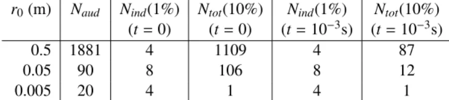
Nind(p), and that by (2) asNtot(p). Some typical values for differentr0’s are shown in Table 3.1. One
may choose either one of two criteria or a combination of both. As indicated in Table 3.1, 8 modes seems sufficient for various sizes of bubble radii using the criterion (1), where theEnfalls below 1%
ofEmax. Therefore, we can also use a fixed number of modes, say 8 to 10, in practice.
Furthermore, recall that in Equation (3.12) the pressure decays exponentially with a rateβn,
where Equation (3.10) tells us thatβnincreases withnand decreases withr0. If we choose to ignore
the initial “burst” and only look at the pressure wave a short time (e.g. 0.001 s) after the creation of
the bubble, then we can drop out even more modes at the beginning. This step is optional and the effect is shown in the rightmost two columns of Table 3.1.
Figure 3.2: A plot of the initial amplitude vs. frequency. From the plot it is clear that as fn (the
frequency of the bubble) approaches 12fb (the damping shifted frequency) the initial amplitude
increases dramatically. We, therefore, use harmonics where fn≈ 12fbbecause they have the largest
r0(m) Naud Nind(1%) Ntot(10%) Nind(1%) Ntot(10%)
(t=0) (t=0) (t=10−3s) (t=10−3s)
0.5 1881 4 1109 4 87
0.05 90 8 106 8 12
0.005 20 4 1 4 1
Table 3.1:Number of modes selected by the two criteria for various typicalr0’s.
propagation in this chapter, we assume a fixed distance between the listener and each bubble using Equations (3.7) and (3.12) to model the pressure at the listener’s ear.
3.1.3 Statistical Generation
In the case where the fluid simulator does not handle bubble generation, we present a statistical approach for generating sound. For a scene at a particular time instant, we consider how many bubbles are created and what they sound like. The former is determined by a bubble generation criteria and the latter is determined by a radius distribution model. As a result, even without knowing the exact motion and interaction of each bubble from the fluid simulator, a statistical approach based on our bubble generation criteria and radius distribution model provide sufficient information for approximating the sound produced in a given scene.
3.1.3.1 Bubble Generation Criteria
Our goal is to examine only the physical and geometrical properties of the simulated fluid, such as fluid velocity and the shape of the fluid surface, and be able to determine when and where a bubble should be generated. Recent works in visual simulation use curvature alone (Narain et al., 2007), or curvature combined with Weber number (Mihalef et al., 2009) as the bubble generation criteria.
In our work, we follow the approach presented by Mihalef et al. (2009). The Weber number is defined as
We= ρ∆U
2L
(σ) (3.13)
beyond a critical value, the gas has sufficient kinetic energy to “break into” the liquid surface and form a bubble; while at lower Weber numbers, the surface tension energy is able to separate the water and air.
Besides the Weber number, we also need to consider the limitation of a fluid simulator. In computer graphics, fluid dynamics is usually solved on a large-scale grid, with small-scale details such as bubbles and droplets added in at regions where the large-scale simulation behaves poorly, namely regions of high curvature. This is because a bubble is formed when the water surface curls back and closes up, at which site the local curvature is high.
Combining the effects of the Weber number and the local geometry, we evaluate the following parameter on the fluid surface
Γ =u2κ, (3.14)
whereuis the liquid velocity andκis the local curvature of the surface. The termu2encodes the Weber number, because in Equation 3.13ρ,σandL(which is taken to be the simulation grid length dx) are constants, and∆U2 = u2 since the air is assumed to be static. Bubbles are generated at regions whereΓis greater than a thresholdΓ0. The criteria also matches what we observe in nature–a
rapid river (largeru) is more likely to trap bubbles than a slow one. In the ocean, bubbles are more likely to form near a wave (largerκ) than on a flat surface–our bubble generation mechanism captures both of these characteristics.
3.1.3.2 Bubble Distribution Model
Once we have determined a location for a new bubble using the generation criteria, we select its radius at random according to a radius distribution model. Works on bubble entrapment by rain (Pumphrey and Elmore, 1990) and ocean waves (Deane and Stokes, 2002) suggest that bubbles are created in a power law (r−α) distribution, whereαdetermines the ratio of small to large bubbles. In nature, theαtakes value from 1.5 to 3.3 for breaking ocean waves (Deane and Stokes, 2002) and≈2.9 for rain (Pumphrey and Elmore, 1990), thus in simulation it can be set according to the scenario. The radius affects both the oscillation frequency (Equation 3.1) and the initial excitation